Effect of the Fermi surface reconstruction on the self-energy of the copper-oxide superconductors

Abstract

We calculated the self-energy corrections beyond the mean-field solution of the rotating antiferromagnetism theory using the functional integral approach. The frequency dependence of the scattering rate ${1}/{\tau}$ is evaluated for different temperatures and doping levels, and is compared with other approaches and with experiment. The general trends we found are fairly consistent with the extended Drude analysis of the optical conductivity, and with the nearly antiferromagnetic Fermi liquid as far as the ${\bf k}$-anisotropy is concerned and some aspects of the Marginal-Fermi liquid behavior. The present approach provides the justification from the microscopic point of view for the phenomenology of the marginal Fermi liquid ansatz, which was used in the calculation of several physical properties of the high-$T_{C}$ cuprates within the rotating antiferromagnetism theory. In addition, the expression of self-energy we calculated takes into account the two hot issues of the high-$T_{C}$ cuprate superconductors, namely the Fermi surface reconstruction and the hidden symmetry, which we believe are related to the pseudogap.

1 Introduction

The origin of the pseudogap (PG) [1] behavior of the high-$T_{C}$ cuprate superconductors (HTSC) remains an open issue even though more than quarter a century has passed after the discovery of superconductivity in these materials [2]. The PG phase turned out to be more challenging and subtle than the superconducting phase itself. Indeed, the PG has been measured as a depression in the density of states at the Fermi energy below the doping dependent PG temperature $T^{*}$, but no broken symmetry has so far been observed beyond any doubt [3]. A number of theoretical models have been proposed in order to explain this PG phenomenon, with some based on the preformed-pairs scenario and others based on competing orders [4]. The rotating antiferromagnetism theory (RAFT), which belongs in the latter, is characterized by two competing orders; namely the d-wave superconductivity and the rotating antiferromagnetic (RAF) order. The RAF order parameter has a finite magnitude below a temperature, which was identified with $T^{*}$, and a phase that varies with time [5, 6, 7, 8, 9, 10]. RAFT yield results in good agreement with several experimental data of the HTSCs. Resistivity [11], optical conductivity [12], Raman [13], and ARPES [14, 9] have been analyzed within RAFT assuming the phenomenological marginal-Fermi liquid (MFL) self-energy [15]. Until before the completion of this work, the justification for using this assumption was missing. The results of this work show that going beyond the mean-field solution of RAFT a self energy that is consistent with a MFL is derived. More importantly, in the limit of the tight-binding bare electrons our self-energy satisfies the same equation as in the second-order Born approximation, which was used in the nearly antiferromagnetic Fermi liquid (NAFL) theory [16]. Moreover, we generalize this approximation into a gapped second-order Born approximation that takes into consideration the PG. Interestingly, we can qualify the RAF state as a state that is nearly antiferromagnetic because the RAF state has the same (free) energy as a true ordered antiferromagnetic state but is a disordered state because of the time dependence of the phase of the RAF order parameter.

Below the PG temperature in the underdoped regime, we find that the relaxation rate displays a linear behavior at large frequencies consistent with a marginal Fermi liquid, but it displays strong deviation from linearity at low frequencies, which is characterized by a hump due to the PG. In the overdoped regime at any temperature or above the PG temperature in the underdoped regime, the relaxation rate shows a mixture of Fermi liquid (FL) and MFL behaviors. We argue that this evolution with doping is related to the Fermi surface (FS) reconstruction [9].

This work is organized as follows. In Sec. 2 we calculate the Gaussian corrections to the mean-field solution of RAFT using a Hubbard-Stratanovich identity that decouples the quartic term of the Hubbard model in the channel of RAF order. This yields the propagator of the Gaussian fluctuations. Self-energy is calculated in Sec. 3 using this propagator, and a gapped second-order Born approximation is derived for self-energy in the presence of the PG. Some numerical results are presented in Sec. 4, and conclusions are drawn in Sec. 5.

2 Method

RAFT has been developed using the extended Hubbard model, with a repulsive on-site Coulomb interaction and a nearest-neighbor attractive interaction that simulates d-wave pairing. Here, we focus on the normal (non superconducting) state, where the Hamiltonian on a two-dimensional lattice reads as

$$H = H_{0}+H_{I}$$ (1)

$$= -t\sum_{\langle i,j\rangle,\sigma}c^{{\dagger}}_{i,\sigma}c_{j,\sigma}-t^{\prime}\sum_{\langle\langle i,j\rangle\rangle,\sigma}c^{{\dagger}}_{i,\sigma}c_{j,\sigma}$$ (3)

$$-\mu\sum_{i,\sigma}c^{{\dagger}}_{i,\sigma}c_{j,\sigma}+U\sum_{i}n_{i,\uparrow}n_{i,\downarrow}.$$

In (1), $H_{0}$ stands for the kinetic and chemical potential energies, and $H_{I}=U\sum_{i}n_{i\uparrow}n_{i\downarrow}$ is the sum of all on-site Coulomb energies. $t$ and $t^{\prime}$ designate the electron’s hopping energies between the nearest-neighbor $(\langle i,j\rangle)$ and next-nearest-neighbor $(\langle\langle i,j\rangle\rangle)$ sites respectively, $\mu$ is the chemical potential, $c^{{\dagger}}_{i,\sigma}$ ($c_{j,\sigma}$) creates (annihilates) an electron with spin $\sigma$ at site $i$, and $n_{i,\sigma}=c^{{\dagger}}_{i,\sigma}c_{i,\sigma}$ is the number operator.

The partition function can be written as [17]

$$Z=\int\prod_{i,\sigma}dc_{i,\sigma}^{*}dc_{i,\sigma}\,e^{-\int_{0}^{\beta}\,d\tau[\Sigma_{i,\sigma}c_{i,\sigma}^{*}\frac{\partial}{\partial\tau}c_{i,\sigma}\,+H_{0}+H_{I}]},$$ (4)

where $c$ and $c^{*}$ are from now on anticommuting Grassmann variables. For the RAF order, we decouple the interacting $U$-term of (1) using a Hubbard-Stratanovich transformation by considering the RAF order parameter $Q=\langle c_{i,\sigma}c^{\dagger}_{i,\sigma}\rangle$, which has been used to model the PG behavior [5, 6]. This gives

$$e^{-\int d\tau H_{I}} = \int\prod_{i}db_{i}\exp\{\int d\tau[-\sum_{i}b_{i}^{*}U^{-1}b_{i}$$ (6)

$$+\sum_{i}c_{i\downarrow}c_{i\uparrow}^{*}b_{i}+\sum_{i}c_{i\uparrow}c_{i\downarrow}^{*}b_{i}^{*}]\},$$

where $b_{i}$ is a Hubbard-Stratanovich complex field. In order to recover the RAF state at the mean-field level in the present treatment we write the field $b_{i}$ as

$$b_{i}=\mid b_{i}\mid e^{i[\pi(x_{i}+y_{i})+\phi(t)]}.$$ (7)

The phase term $e^{i\pi(x_{i}+y_{i})}=(-1)^{x_{i}+y_{i}}$ guarantees that the rotating order parameter is staggered due to the antiferromagnetic correlations, and the time-dependent phase $\phi(t)$ insures that the staggered magnetization rotates [10, 12, 6, 7]. Using the Grassmann variables and the transformation (6), the partition function takes on the form

$$Z=\int\prod_{i,\sigma}dc_{i,\sigma}^{*}dc_{i,\sigma}db_{i}\exp(-S_{eff}),$$ (8)

with

$$S_{eff} =\int_{0}^{\beta}\,d\tau[\sum_{i\sigma}\sum_{\alpha=A,B}{c_{i\sigma}^{\alpha^{*}}\frac{\partial}{\partial\tau}c_{i,\sigma}^{\alpha}}+H_{0}^{\alpha}$$ (10)

$$+\sum_{i;\alpha=A,B}(c_{i\uparrow}^{\alpha^{*}}c_{i\downarrow}^{\alpha}b_{i}+c_{i\downarrow}^{\alpha^{*}}c_{i\uparrow}^{\alpha}b^{*}_{i})+\sum_{i}\frac{\mid b_{i}\mid^{2}}{U}].$$

Here $\beta=\frac{1}{k_{B}T}$ is inverse temperature, and $A$ and $B$ designate the two sublattices of the bipartite lattice. The upper index $\alpha$ in $H_{0}^{\alpha}$ means that the single particle part of the Hamiltonian has now to be written using the two sublattices, $A$ and $B$. The mean-field solution, where $b_{i}\equiv b_{0}$ is time and space independent, allows us to recover the RAFT’s mean field equation for the parameter $Q=|\langle c_{i,\uparrow}c_{i,\downarrow}^{\dagger}\rangle|$, Ref. [5]:

$$1=\frac{U}{2N}\sum_{\bf k}\frac{n_{F}[E_{-}({\bf k})]-n_{F}[E_{+}({\bf k})]}{E_{q}({\bf k})},$$ (11)

where $n_{F}(E)=\frac{1}{1+e^{\beta E}}$, $E_{q}({\bf k})=\sqrt{\epsilon_{1}({\bf k})^{2}+b_{0}^{2}}$, and $N$ is the total number of lattice sites. The mean field energies $E_{\pm}=-\mu^{\prime}({\bf k})\,\pm\,E_{q}({\bf k})$ are the same as those derived earlier in Ref. [5] when we let $b_{0}=UQ$; $Q$ being then the RAF order parameter satisfying Eq. (11). Here, $\epsilon_{1}({\bf k})=-2t(\cos k_{x}+\cos k_{y})$ and $\mu^{\prime}({\bf k})=-\mu-4t^{\prime}\cos k_{x}\cos k_{y}+Un$. $n=\langle c_{i\sigma}\rangle$ is the electron’s density, which satisfies the following mean-field equation [5]

$$n = \frac{1}{2N}\sum_{\bf k}{n_{F}[E_{+}({\bf k})]+n_{F}[E_{-}({\bf k})]}.$$ (12)

Note that the decoupling the quartic interacting term of the Hubbard Hamiltonian using this density order parameter led to adding $Un$ in the expression of $\mu^{\prime}({\bf k})$, [5]. The fluctuations beyond the mean-field solution are considered for the RAF order only for simplicity. Also, the fluctuations considered here are in the longitudinal direction of the RAF parameter, since we argue that these are much more important than the transverse fluctuations, given that the phase of the local RAF parameter is time dependent, so already fluctuating at the mean-field level.

Upon Fourier transforming to ${\bf k}$ and frequency space, the mean-field action takes on the form

$$S_{0}=\sum_{\tilde{k}}\psi_{\tilde{k}}^{*}{\cal G}^{-1}\psi_{\tilde{k}}+N\frac{\mid b\mid^{2}}{U},$$ (13)

where ${\tilde{k}}\equiv({\bf k},\omega_{n})$; ${\bf k}$ being the wavevector and $\omega_{n}$ the fermionic Matsubara frequency. Here, $\psi_{\tilde{k}}^{*}=(c_{{\tilde{k}}\uparrow}^{A^{*}}\ c_{{\tilde{k}}\uparrow}^{B^{*}}\ c_{{\tilde{k}}\downarrow}^{A^{*}}\ c_{{\tilde{k}}\downarrow}^{B^{*}})$ is a 4-component spinor, and the mean-field Green’s function is [11]

$${\cal G}({\bf k},i\omega_{n})=\frac{[i\omega_{n}+\mu^{\prime}({\bf k})]I+\epsilon({\bf k}){\cal M}+b{\cal N}}{[i\omega_{n}+\mu^{\prime}({\bf k})]^{2}-[\epsilon^{2}({\bf k})+b^{2}]},$$ (14)

with

$$\mathcal{\cal M}=\left(\begin{array}[]{cc}\tau_{1}&0\\ 0&\tau_{1}\end{array}\right),\ \ \ \ \mathcal{\cal N}=\left(\begin{array}[]{cc}0&\tau_{3}\\ \tau_{3}&0\end{array}\right),$$ (19)

where $\tau_{1}$ and $\tau_{3}$ are the first and third Pauli matrices.

In order to go beyond the mean-field solution, we consider the Gaussian fluctuations by writing

$$b_{i}=b_{0}+\delta b({\bf{r_{i}}},\tau),$$ (20)

with $\delta b({\bf{r_{i}}},\tau)$ a small deviation around the mean-field point. Using the approach for calculating Gaussian contributions to the partition function described in Ref. [17] one finds

$$Z=Z_{0}\,\int\prod_{i}d(\delta b_{i})\exp\bigg{(}-\frac{1}{2}\int_{0}^{\beta}\,d\tau\sum_{i}\delta b_{i}\Gamma^{-1}\delta b_{i}^{*}\bigg{)},$$ (21)

where $Z_{0}$ is the mean-field partition function, and $\Gamma$ the propagator of the Gaussian fluctuations, given in Fourier space by

$$\Gamma({\tilde{q}})=\frac{2U}{1-{U}\chi({\tilde{q}})/4}.$$ (22)

The particle-hole type bubble $\chi$ reads as

$$\chi({\tilde{q}}) = \sum_{\omega_{n}}\int\frac{d^{2}k}{(2\pi)^{2}}{\rm Tr}[{\cal G}({\tilde{k}})\,{\cal N}{\cal G}({\tilde{k}}+{\tilde{q}})\,{\cal N}]$$ (23)

$$= \int\frac{d^{2}k}{(2\pi)^{2}}\frac{d\epsilon d\epsilon^{\prime}}{(2\pi)^{2}}\frac{n_{F}(\epsilon)-n_{F}(\epsilon^{\prime})}{\epsilon-\epsilon^{\prime}+i\omega_{m}}$$ (25)

$${\rm Tr}[A({\bf k},\epsilon){\cal N}A({\bf k}+{\bf q},\epsilon^{\prime}){\cal N}].$$

where ${\tilde{q}}\equiv({\bf q},i\omega_{m})$; $\omega_{m}$ being the bosonic Matsubara frequency, and ${\rm Tr}$ designates the trace of a matrix. The spectral function $A({\bf k},\epsilon)$ is related to the Green’s function by ${\cal G}({\bf k},i\omega_{n})=\int\frac{d\epsilon}{2\pi}\frac{A({\bf k},\epsilon)}{i\omega_{n}-\epsilon}$. The imaginary part of $\chi$, which is needed in the calculation of the imaginary part of the self-energy, is

$$\chi^{\prime\prime}(q,\omega) = \int\frac{d^{2}k}{(2\pi)^{2}}\frac{d\epsilon}{4\pi}[n_{F}(\epsilon)-n_{F}(\epsilon+\omega)]{\rm Tr}[A({\bf k},\epsilon){\cal N}A({\bf k}+{\bf q},\epsilon+\omega){\cal N}]$$ (26)

$$\approx \int\frac{d{\bf k}}{(2\pi)^{2}}\frac{\omega}{\pi}\sum_{s=\pm}\sum_{s^{\prime}=\pm}C_{ss^{\prime}}({\bf k},{\bf q})\frac{\eta}{[\mu^{\prime}({\bf k})+sE_{q}({\bf k})]^{2}+\eta^{2}}$$ (28)

$$\times\frac{\eta}{[\omega+\mu^{\prime}({\bf k}-{\bf q})+s^{\prime}E_{q}({\bf k}-{\bf q})]^{2}+\eta^{2}}$$

where

$$C_{ss^{\prime}}({\bf k},{\bf q})=1+ss^{\prime}\frac{U^{2}Q^{2}-\epsilon({\bf k})\epsilon({\bf k}-{\bf q})}{E_{q}({\bf k})E_{q}({\bf k}-{\bf q})}.$$

In (28), we used $n_{F}(\epsilon)-n_{F}(\epsilon+\omega)\approx\omega\delta(\epsilon)$ in the low frequency and low temperature regime. In order to derive an expression for $\chi^{\prime\prime}$ consistent with a memory function-like approximation [18, 19], the $\omega$ independent Lorentzian in (28) is replaced by a delta function in the limit $\eta\to 0$: $\frac{\eta}{[\mu^{\prime}({\bf k})+sE_{q}({\bf k})]^{2}+\eta^{2}}\approx\pi\delta(\mu^{\prime}({\bf k})+sE_{q}({\bf k})).$ This constrains the integration over ${\bf k}$ to be performed over the FS, which satisfies $\mu^{\prime}({\bf k})+sE_{q}({\bf k})=0$ with $s=\pm$; Ref. [14]. With this, $\chi^{\prime\prime}$ assumes the simpler form

$$\chi^{\prime\prime}(q,\omega)=\int_{FS}\frac{d{\bf k}}{(2\pi)^{2}}\sum_{s,s^{\prime}}$$ (29)

$$\frac{C_{ss^{\prime}}({\bf k},{\bf q})\omega\eta}{[\omega+\mu^{\prime}({\bf k}-{\bf q})+s^{\prime}E_{q}({\bf k}-{\bf q})]^{2}+\eta^{2}}.$$ (30)

The integral in (30) runs over points belonging in the FS, only. In the high temperature limit or in the overdoped regime, the FS in RAFT consists of large contours around $(0,0)$ and $(\pi,\pi)$ [9, 13]. Also the FS surface in this case is characterized by significant nesting for momenta transfers slightly different than $(\pi,\pi)$ [13, 9]. This nesting property is significantly reduced in the underdoped regime below $T^{*}$, because the FS reconstructs into small hole pockets around the points $(\pm\pi/2,\pm\pi/2)$ [13, 9]. The presence of the PG in this case also reduces the density of states for wavevectors on the FS. These facts will cause $\chi^{\prime\prime}$ to be greater in the overdoped regime and for temperatures greater than $T^{*}$ in the underdoped regime in general. This behavior of $\chi^{\prime\prime}$ will affect the doping and temperature dependence of self-energy as explained next.

3 Derivation of self-energy in the presence of the PG

Using the Feynman diagram for self-energy depicted in Fig. 1, we write

$$\Sigma({\tilde{k}})=2T\int\,\frac{d^{2}q}{(2\pi)^{2}}\,\sum_{\omega_{m}}{\cal G}({\tilde{k}}-{\tilde{q}})\,\Gamma({\tilde{q}}).$$ (31)

In order to carry on the calculations for self-energy we expend $\Gamma({\tilde{q}})$ to second order in $U$ in the limit of $U<W$, with $W$ being the bare bandwidth energy ($W=8t$ if $t^{\prime}=0$). Keeping only the lowest-order term contributing to the imaginary part of self-energy one gets

$$\Sigma({\tilde{k}}) \approx U^{2}\int\frac{d^{2}q}{(2\pi)^{2}}\frac{d^{2}k^{\prime}}{(2\pi)^{2}}\frac{d\epsilon}{2\pi}\frac{d\epsilon^{\prime}}{2\pi}\frac{d\epsilon^{{}^{\prime\prime}}}{2\pi}\Delta n_{F}A({\bf k}-{\bf q},\epsilon^{{}^{\prime\prime}})$$

$$\times{\rm Tr}[A({\bf k}^{\prime},\epsilon){\cal N}A({\bf k}^{\prime}+{\bf q},\epsilon^{\prime}){\cal N}]\frac{n_{F}(-\epsilon^{{}^{\prime\prime}})+n_{B}(\epsilon^{\prime}-\epsilon)}{i\omega_{n}-\epsilon^{{}^{\prime\prime}}-\epsilon^{\prime}+\epsilon},$$

where $\Delta n_{F}=n_{F}(\epsilon)-n_{F}(\epsilon^{\prime})$, and $n_{B}$ is the Einstein-Bose factor. Taking the analytical limit $i\omega_{n}\longrightarrow\omega+i0^{+}$ gives the following expression for the imaginary part of self-energy:

$$\Sigma^{\prime\prime}({\bf k,\omega}) = U^{2}\int\frac{d^{2}q}{(2\pi)^{2}}\frac{d^{2}k^{\prime}}{(2\pi)^{2}}\frac{d\epsilon d\epsilon^{\prime}}{8\pi^{2}}[{n_{F}(\epsilon^{\prime}-\epsilon-\omega)+n_{B}(\epsilon^{\prime}-\epsilon)}]$$ (35)

$$\Delta n_{F}A({\bf k}-{\bf q},\epsilon-\epsilon^{\prime}+\omega){\rm Tr}[A({\bf k}^{\prime},\epsilon){\cal N}A({\bf k}^{\prime}+{\bf q},\epsilon^{\prime}){\cal N}].$$

In the limit of the tight-binding electrons where the PG is absent, so with $A({\bf k}-{\bf q},\epsilon-\epsilon^{\prime}+\omega)\approx 2\pi\delta(\omega+\epsilon-\epsilon^{\prime}-\epsilon_{{\bf k}-{\bf q}})$, Eq. (35) is shown to reduce to the same expression as in the second-order Born approximation used in NAFL [16], namely:

$$\Sigma^{\prime\prime}({\bf k},\omega)\approx g^{2}\int\frac{d^{2}k^{\prime}}{4\pi^{2}}\chi^{\prime\prime}({\bf k}-{\bf k}^{\prime},\omega-\epsilon_{{\bf k}^{\prime}})[{n_{F}(\epsilon_{{\bf k}^{\prime}})+n_{B}(\epsilon_{{\bf k}^{\prime}}-\omega})],$$ (36)

where $g=U$ in the present intermediate coupling regime.

It is possible to derive a Born approximation that incorporates the PG effect using the mean-field result for the spectral function. The latter is obtained from the Green’s function (14) through $A({\bf k},\omega)=-2{\rm Im}G({\bf k},\omega)$; Ref. [11]:

$$A({\bf k},\omega)=\sum_{s=\pm}\frac{\eta}{[\omega+\mu^{\prime}({\bf k})+sE_{q}({\bf k})]^{2}+\eta^{2}}a_{s}({\bf k})$$ (37)

with $a_{s}({\bf k})=I-s\big{[}\frac{\epsilon({\bf k})}{E_{q}({\bf k})}{\cal M}+\frac{UQ}{E_{q}({\bf k})}{\cal N}\big{]}$. $I$ is the $4\times 4$ identity matrix. Taking $\eta\to 0^{+}$ gives

$$A({\bf k},\omega) = \pi\sum_{s=\pm}\delta\bigg{(}\omega+\mu^{\prime}({\bf k})+sE_{q}({\bf k})\bigg{)}a_{s}({\bf k}).$$ (38)

The Dirac delta function in (38) allows the integration over $\epsilon^{\prime}$ in (35) to be readily performed. This results in a much simpler expression for the imaginary part of self-energy:

$$\Sigma^{\prime\prime}({\bf k,\omega}) = \sum_{s=\pm}U^{2}\int\frac{d^{2}{k}^{\prime}}{(2\pi)^{2}}a_{s}({\bf k}^{\prime})\chi^{\prime\prime}\big{(}{\bf k}-{\bf k}^{\prime},\omega-E_{s}({\bf k}^{\prime})\big{)}$$ (40)

$$[n_{F}\big{(}E_{s}({\bf k}^{\prime})\big{)}+n_{B}\big{(}E_{s}({\bf k}^{\prime})-\omega\big{)}].$$

There are two noticeable effects for the PG on self-energy. First, the tight-binding energies in the Fermi and Bose factors as well as in $\chi^{\prime\prime}$ are replaced by RAFT’s eigenenergies $E_{\pm}({\bf k})$. Second, the self-energy becomes a matrix when the PG is present, with the off-diagonal elements caused by the terms proportional to the matrices ${\cal M}$ and ${\cal N}$ in the RAFT’s spectral function (38).

As it is extremely difficult to calculate $\Sigma^{\prime\prime}$ analytically due to the double integral over ${\bf k}$ and to the dependence on $\chi^{\prime\prime}$, which is itself difficult to calculate analytically, we performed this calculation numerically. Note that Stojkovic and Pines [16] calculated analytically $\Sigma^{\prime\prime}$ in the absence of the PG using the gapless second-order Born approximation in Eq. (36). They found that the ${\bf k}$-averaged scattering rate takes on the MFL form. In our case, we also get this MFL behavior in addition to other effects due to the PG, which were not included in Stojkovic and Pines’ work.

4 Results

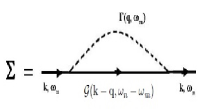
Figure 1: The leading order self-energy diagram is drawn. The dashed line is the propagator ${\Gamma}$ of the Gaussian fluctuations beyond the mean-field solution. The continuous line is the propagator ${\cal G}$ of the quasi-particles in the mean-field solution.

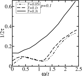
Figure 2: $1/2\tau=-\Sigma^{\prime\prime}$ is plotted versus $\omega$ for the wavevector $(k_{x},k_{y})=(k_{F},k_{F})\in$ FS with $k_{F}=0.4\pi$. Temperature and doping are indicated on the figure. The Hamiltonian parameters used in the present work are $U=3t$ and $t^{\prime}=-0.16t$. All numerical calculations were performed on a $100\times 100$ Brillouin zone, and a mesh of $100\times 100$ points for the momentum transfer. Here, ${\bf k}=(0.4\pi,0.4\pi)$ along the diagonal. $1/\tau$ is in units of $t$.

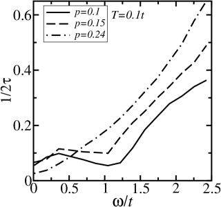
Figure 3: $1/2\tau=-\Sigma^{\prime\prime}$ is drawn versus frequency $\omega$ for three values of doping at temperature $T=0.1t$. Here, ${\bf k}=(k_{F},k_{F})\in$ FS along the diagonal, with $k_{F}=0.4\pi$. Note that the Fermi wavevector does not change significantly with doping along the diagonal.

Figure 2 displays ${1}/{2\tau}=-\Sigma^{\prime\prime}$ versus the frequency $\omega/t$ for the wavevector ${\bf k}_{F1}=(0.4\pi,0.4\pi)$ on the FS and for three different temperatures and a fixed doping $p=0.1$. The Hamiltonian parameters are $U=3t$, and $t^{\prime}=-0.16t$. Here, for the sake of simplicity, we focus only on the diagonal elements of the self-energy, which are all equal. At the highest temperature $T=0.3t$, ${1}/{2\tau}$ shows a mixture of FL and MFL behaviors. $1/2\tau$ can be fitted using linear and quadratic terms in $\omega/t$. The linear frequency dependence (MFL) is a consequence of the nesting property of the FS. There is no PG at this temperature, and the FS consists of large contours around $(0,0)$ and $(\pi,\pi)$. For lower temperatures ($T=0.1t$ and $T=0.05t$), the PG is present, and the FS reconstructs into pockets around $(\pm\pi/2,\pm\pi/2)$ [9, 14]. The nesting surface shrinks and the number of quasiparticle states available in the system becomes smaller. The first consequence of the nesting decrease is to reduce ${1}/{2\tau}$ by roughly a factor $2$ at high frequencies. At low frequencies, the electron-electron scattering processes are reduced because of the depletion of the density of states at the Fermi energy due to the PG, and the quasiparticle lifetime $\tau$ increases. This effect is more pronounced at lower temperature.

Figure 3 displays ${1}/{2\tau}$ versus $\omega/t$ for different doping values at the temperature $T=0.1t$ and for the wavevector ${\bf k}_{F1}=(0.4\pi,0.4\pi)$ on the FS. In the underdoped regime with $p=0.1$ and $0.15$, ${1}/{2\tau}$ shows a linear behavior at high values of $\omega/t$ and a downward deviation at lower frequencies, which occurs at a value of $\omega/t$ that increases when doping decreases. This is a signature of the PG, which is bigger at lower doping. For $p=0.24$ in the overdoped regime, ${1}/{2\tau}$ can be fitted by linear and quadratic terms in $\omega/t$. Again, this is a mixture of FL and MFL behaviors, but ${1}/{2\tau}$ goes to a lower value when $\omega/t$ tends to zero indicating a greater FL tendency.

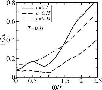
Figure 4: $1/2\tau=-\Sigma^{\prime\prime}$ is drawn versus frequency $\omega$ for three values of doping at temperature $T=0.1t$ and for wavevectors on the FS. The wavevectors are ${\bf k}=(0.47\pi,0.41\pi)$ for $p=0.1$, ${\bf k}=(0.74\pi,0.71\pi)$ for $p=0.15$, and ${\bf k}=(0.45\pi,0.4\pi)$ for $p=0.24$. Here, the Fermi wavevector changes significantly with doping away from the diagonal.

In figure 4, $1/2\tau$ is drawn versus $\omega/t$ for three doping levels and for wavevectors on the FS away from the diagonal of the Brillouin zone. Due to the FS reconstruction with doping, these wavevectors are different for different dopings. First of all, it is clear from this figure and figure 3 that $1/2\tau$ shows a strong ${\bf k}$ dependence. For example, for $p=0.1$ in the underdoped regime, there is a factor of $2$ roughly between $1/2\tau$ for the FS point away from the diagonal (Fig. 4) and the FS point on the diagonal (Fig. 3). For this doping ($p=0.1$), the MFL linear behavior at high frequencies is followed by a deviation from linearity as the frequency decreases, then by a hump due to the PG at even lower frequencies. For $p=0.15$ near the optimal point, $1/2\tau$ decreases linearly with frequency, then saturates for $\omega\leq t$ and presents a hump due to the PG at even lower frequency. These trends are the same as those encountered for the FS point on the diagonal of the Brillouin zone in Fig. 3. For the doping $p=0.24$ above the optimal point (where the PG is zero), $1/2\tau$ can be fitted using linear and quadratic terms; it thus shows a mixture of FL and MFL behavior like for the FS point on the diagonal.

Regarding the comparison with experiment, our results for self-energy are qualitatively consistent with the experimental data of the optical conductivity, which was analyzed using the extended Drude model [1]. The downward deviation from linearity in $1/2\tau$ versus frequency, observed experimentally, is accounted for in the present theory. Taking $t=0.1$ eV, which is the value considered in RAFT’s past works, we find that the values of $1/\tau$ are in the same range as the experimental ones [1]. Note that $1/2\tau$ is in units of $t$ in figures 2, 3, and 4. There are however discrepancies between the calculated relaxation rate and the experimental one. These differences can be attributed mainly to the following reasons: the extended Drude analysis used the Drude conductivity with a mass enhancement factor and a frequency and temperature dependent relaxation rate. This analysis does not take into account the PG explicitly, contrary to the present microscopically calculated self-energy, which does include the PG. Also, in RAFT, the establishment of the PG below $T^{*}$ in the underdoped regime causes the reconstruction of the FS. This important property is not unfortunately taken into account in the extended Drude analysis. Note that our present approach does not consider the contributions of the real part of self-energy in this comparison with the extended Drude analysis.

5 Conclusions

In order to justify the usage of a MFL-like self-energy in past works based on RAFT, we calculated the self-energy corrections beyond the mean-field solution of this theory, and found that the doping, temperature and frequency dependences of this self-energy agree qualitatively well with the results of the nearly antiferromagnetic Fermi liquid as far as this MFL behavior is concerned. Also, the trends of the imaginary part of this self-energy capture well the main features of the relaxation rate derived in the extended Drude analysis of the optical conductivity. Note that, contrary to that analysis, the expression of self energy in the present work depends explicitly on the pseudogap. The main consequences of the latter are a deviation from linearity and a hump in the low frequency regime in the frequency dependence of the relaxation rate $1/\tau$. According to the present results, the changes in the frequency dependence of self-energy as doping goes from the overdoped regime to the underdoped regime are due to the reconstruction of the Fermi surface near optimal doping.

References

- [1] T. Timusk, B. Statt, Rep. Prog. Phys. 62, 61 (1999).
- [2] J.G. Bednorz and K.A. Mueller, Z. Phys. B- Condensed Matter 64, 189 (1986).
- [3] Rui-Hua He, M. Hashimoto, H. Karapetyan, J.D. Koralek, J.P. Hinton, J.P. Testaud, V. Nathan, Y. Yoshida, Hong Yao, K. Tanaka, W. Meevasana, R.G. Moore, D. H. Lu, S.-K. Mo, M. Ishikado, H. Eisaki, Z. Hussain, T.P. Devereaux, S.A. Kivelson, J. Orenstein, A. Kapitulnik, Z.-X. Shen, Science 331, 1579 (2011).
- [4] S. Chakravarty, R. B. Laughlin, D. K. Morr, and C. Nayak, Phys. Rev. B 63, 094503 (2001). This paper proposed the so-called DDW order to be in competition with d-wave superconductivity.
- [5] M. Azzouz, Phys. Rev. B 67, 134510 (2003).
- [6] M. Azzouz, Phys. Rev. B 68, 174523 (2003).
- [7] M. Azzouz, Phys. Rev. B 70, 052501 (2004).
- [8] M. Azzouz, Physica C 480, 34 (2012).
- [9] M. Azzouz, Spectrum 5, 215 (2013).
- [10] M. Azzouz, in preparation (2013).
- [11] H. Saadaoui and M. Azzouz, Phys. Rev. B 72, 184518 (2005).
- [12] E.H. Bhuiyan, G. Presenza-Pitman, M. Azzouz, Physica C 473, 61 (2012).
- [13] M. Azzouz, K.C. Hewitt, H. Saadaoui, Phys. Rev. B 81, 174502 (2010).
- [14] M. Azzouz, B.W. Ramakko, G. Presenza-Pitman, J. Phys.: Condens. Matter 22, 345605 (2010).
- [15] C. M. Varma, P. B. Littlewood, and S. Schmitt-Rink, E. Abrahams and A. E. Ruckenstein, Phys. Rev. Lett. 63, 1996 (1989)
- [16] B.P. Stojkovic and D. Pines, Phys. Rev. B 56, 11931 (1997).
- [17] J.W. Negele and H. Orland, Quantum Many-Particle Systems, Addison-Wesley Publishing Company (1988).
- [18] M. Opel, R. Nemetschek, C. Hoffman, R. Philipp, P.F. Mller, R. Hackl, I. Ttto, A. Erb, B. Revaz, E. Walker, H. Berger, and L. Forró, Phys. Rev. B 61, 9752 (2000).
- [19] W. Gtze and P. Wlfe, Phys. Rev. B 6, 1226 (1972).