Nonequilibrium fluctuation-dissipation theorem and heat production

Abstract

We use a relationship between response and correlation function in nonequilibrium systems to establish a connection between the heat production and the deviations from the equilibrium fluctuation-dissipation theorem. This scheme extends the Harada-Sasa formulation [Phys. Rev. Lett. 95, 130602 (2005)], obtained for Langevin equations in steady states, as it also holds for transient regimes and for discrete jump processes involving small entropic changes. Moreover, a general formulation includes two times and the new concepts of two-time work, kinetic energy, and of a two-time heat exchange that can be related to a nonequilibrium “effective temperature”. Numerical simulations of a chain of anharmonic oscillators and of a model for a molecular motor driven by ATP hydrolysis illustrate these points.

For systems in equilibrium, the response $R$ to a small external perturbation is related to the correlation function $C$ of spontaneous fluctuations. This property is described by the fluctuation-dissipation theorem (FDT). In the last two decades, many efforts have been devoted to the study and the understanding of deviations from FDT in nonequilibrium systems Crisanti and Ritort (2003); Marini Bettolo Marconi et al. (2008); Seifert and Speck (2010); Baiesi and Maes (2013). These studies can be substantially split in two research lines: i) establishing a connection between deviations from FDT and thermodynamic properties; ii) searching for general relations including $R$ and $C$ that hold also out of equilibrium.

Along the first line there is the definition of an effective temperature in nonequilibrium systems, based on the formula of the equilibrium FDT and coinciding with the temperature $T$ of the thermal bath if the FDT holds Cugliandolo et al. (1997). The concept of effective temperature has been introduced in a variety of systems including aging or driven systems and quantum quenches Cugliandolo (2011). More recently Harada and Sasa (HS) have derived a relation between the average rate of energy dissipation $J$ and deviations from the FDT Harada and Sasa (2005, 2006); Harada (2009), for systems described by a Langevin equation with white noise (see also the extension to colored noise Deutsch and Narayan (2006)). Indicating with $C$ the velocity correlation function and with $R$ the change of velocity caused by a constant external force, the HS relation reads

$${\left\langle{J}\right\rangle}=\gamma\int_{-\infty}^{\infty}[\tilde{C}(\omega)-2T\tilde{R}_{S}(\omega)]\frac{d\omega}{2\pi},$$ (1)

where $\langle\dots\rangle$ denotes an average over trajectories. The friction coefficient $\gamma$ is related to the typical inverse time of energy dissipation. Quantities in Fourier space are denoted with a tilde, and $\tilde{R}_{S}(\omega)$ is the transform of the symmetric part $R_{S}(t)$ of the response function (i.e. the real part of the transform). The advantage of this approach is that correlation functions and response functions of fluctuating observables are often more easily accessible in experiments and one can thus utilize deviations from FDT to indirectly infer the rate of energy dissipation (see also a recent alternative Lander et al. (2012)). For example, it was utilized to study optically driven colloidal systems Toyabe et al. (2007) and the energetics of a model for molecular motor Toyabe et al. (2010). Although it was originally obtained for nonequilibrium steady states, the formula (1) was also used in the microrheology of a particle trapped in a relaxing lattice Gomez-Solano et al. (2012).

Concerning the research line (ii), many expressions of $R$ in terms of quantities of the unperturbed dynamics have been proposed in the last years for a wide range of nonequilibrium systems (see for example Cugliandolo et al. (1994); Lippiello et al. (2005); Speck and Seifert (2006); Baiesi et al. (2009); Gomez-Solano et al. (2009) and references in Crisanti and Ritort (2003); Marini Bettolo Marconi et al. (2008); Seifert and Speck (2010); Baiesi and Maes (2013)). In this letter we will focus on the following generalized FDT (GFDT) Lippiello et al. (2005); Baiesi et al. (2009). Indicating with $R=\partial{\left\langle{Z(t_{2})}\right\rangle}/\partial h(t_{1})|_{h=0}$ the response of an observable $Z$ to an external perturbation $h$ coupled with the observable $Y$, and fixing $t_{2}\geq t_{1}$, the GFDT reads

$$2TR(t_{1},t_{2})=\frac{\partial{\left\langle{Z(t_{2})Y(t_{1})}\right\rangle}}{\partial t_{1}}-{\left\langle{Z(t_{2})B(t_{1})}\right\rangle}$$ (2)

where the observable $B$ satisfies the relation

$${\left\langle{B(t_{2})Z(t_{1})}\right\rangle}=\frac{\partial{\left\langle{Y(t_{2})Z(t_{1})}\right\rangle}}{\partial t_{2}}$$ (3)

for any $Z$. This GFDT holds for systems described by Markovian dynamics, under quite general assumptions Lippiello et al. (2005); Baiesi et al. (2009).

In this Letter we present a connection between the GFDT (2) and the HS relation (1). More precisely we prove that a relation between heat flux, response function, and velocity correlation holds a) not only for steady states but in general transients; b) for general discrete variables evolving according to jump processes, such as particle collisions or the positions in a discrete space; c) not only on average but also for suitably defined fluctuating parts of $C$, $R$ and $J$. Our framework includes novel quantities: a “two-time” generalized heat, a “two-time” kinetic energy and a “retarded-anticipated” work. The GFDT allows one to find a connection between these “two-time” observables and eventually to support the definition of an effective temperature from FDT deviations in systems where timescales corresponding to different degrees of freedom are well-separated.

We consider a system of $N$ particles and indicate with ${\bf x}_{i}(t),{\bf v}_{i}(t)$ the position and velocity of the $i$-th particle at time $t$ and with $m_{i}$ its mass. Each particle is affected by a force ${\bf f}_{i}(t)$ that is the sum of internal and external interactions and that can be non-conservative. We first develop an approach where time is discretized with fixed time step $\tau$ and the local velocity $v_{i}(t)$ can be updated to a new value $v^{\prime}_{i}(t)$ with a stochastic evolution characterized by transition rates $\Omega(v_{i}(t)\to v^{\prime}_{i}(t))$, while positions follow deterministically $x_{i}(t+\tau)=x_{i}(t)+v^{\prime}_{i}(t)\tau$. Such approach can reproduce Langevin inertial dynamics. Later we will shift the attention to discrete-state systems where positions change stochastically and velocities are subordinate variables. Within this formalism time derivatives are discrete: $\tau\partial v_{i}(t)/\partial t=\delta v_{i}(t)$ and $\tau\partial x_{i}(t)/\partial t=\delta x_{i}(t)$. To simplify the notation hereafter we restrict to a one-dimensional motion and we drop the particle index, the generalization to more variables being trivial for quantities with uncorrelated fluctuations.

A “two-time” kinetic energy and an elementary retarded-anticipated work Zamponi et al. (2005) during $\tau$ are defined as

$$\hat{K}(t_{1},t_{2}) \equiv \frac{m}{2}v(t_{2})v(t_{1})$$ (4)

$$\delta\hat{W}(t_{1},t_{2}) \equiv \frac{1}{2}\tau\left[f(t_{2})v(t_{1})+v(t_{2})f(t_{1})\right]\,.$$ (5)

The notation $\hat{X}(t)$ is useful to explicitly indicate fluctuating quantities, namely $X(t)=\langle\hat{X}(t)\rangle$ (however, positions and velocities are always meant to be fluctuating). In the $t_{2}\to t_{1}$ limit, $\hat{K}$ and $\hat{W}$ coincide with the standard definition of kinetic energy and work. Moreover, for an isolated system not coupled with a thermal reservoir — where $f(t)=m\ \delta v(t)/\tau$ — it is easy to show that they satisfy a Work-Energy theorem for arbitrary $t_{2}$ and $t_{1}$,

$$\delta\hat{W}(t_{1},t_{2})=\frac{m}{2}\left[\delta v(t_{2})v(t_{1})+v(t_{2})\delta v(t_{1})\right]=d\hat{K}(t_{1},t_{2}).$$ (6)

It is therefore natural to define the “two-time heat exchange” (from the reservoir to the system) as

$$\delta\hat{Q}(t_{1},t_{2})\equiv d\hat{K}(t_{1},t_{2})-\delta\hat{W}(t_{1},t_{2}).$$ (7)

The two-time kinetic energy is trivially proportional to the velocity-velocity fluctuations, namely $\hat{C}(t_{1},t_{2})\equiv v(t_{2})v(t_{1})$. Notice that our definition of heat is related to Eq. (59) of Ref. Harada and Sasa (2006) (written for Langevin equations at stationarity), and in the limit of equal times it has the structure of the heat defined in stochastic energetics Sekimoto (2010). One can express $\delta\hat{W}$ in terms of the velocity correlation function $\hat{C}(t_{1},t_{2})$ and of a “fluctuating” response function $\hat{R}(t_{1},t_{2})$ of the velocity $v(t_{2})$ to an external force switched on during the microscopic time interval $[t_{1},t_{1}+\tau]$ (see below).

Observing that the external force $h(t_{1})$ perturbs the system energy by a factor $h(t_{1})v(t_{1})\tau$, the response function $R(t_{1},t_{2})$ can be immediately obtained putting $Z(t_{2})=v(t_{2})$ and $Y(t_{1})=v(t_{1})\tau$ in Eqs (2,3), which for discrete time dynamics read

$$2TR(t_{1},t_{2}) = {\left\langle{v(t_{2})\delta v(t_{1})}\right\rangle}-{\left\langle{v(t_{2})\hat{B}(t_{1})}\right\rangle}$$ (8)

$${\left\langle{\hat{B}(t_{2})v(t_{1})}\right\rangle} = {\left\langle{\delta v(t_{2})v(t_{1})}\right\rangle}.$$ (9)

The next step is to express $\hat{B}$ in terms of system properties. For simplicity, in this derivation we allow variations of $v\to v^{\prime}=v\pm\epsilon$. Since velocities evolve with jumps, we have Lippiello et al. (2005); Baiesi et al. (2009)

$$\hat{B}(t)=\epsilon\tau\left[\Omega(v\to v+\epsilon)-\Omega(v\to v-\epsilon)\right]$$ (10)

and, assuming local equilibrium, transition rates $\Omega(v\to v^{\prime})$ embody the property of local (or generalized) detailed balance Lebowitz and Spohn (1999); Maes (1999),

$$\Omega(v\to v+\epsilon)=\alpha(\epsilon)e^{[dS(v+\epsilon)-dS(v)]/2},$$ (11)

where $dS(v+\epsilon)-dS(v)$ is the additional entropy change in the environment caused by the velocity jump and $\alpha(\epsilon)$ is a symmetric function of $\epsilon$ fixing the jump rates. For systems in contact with a single heat bath with $\beta=1/T$ (setting the Boltzmann constant $k_{B}=1$), the entropy change should take the form $dS(t)=-\beta\,\delta\hat{Q}(t,t)$ with the heat transferred defined in Eq. (7) leading to

$$dS(v+\epsilon)-dS(v)=-\beta\epsilon[mv-f\tau].$$ (12)

With this equation, and assuming that $\zeta\equiv\beta m\epsilon^{2}\ll 1$ one expands the exponential in Eq. (11) to find $\hat{B}(t)=-\alpha(\epsilon)\zeta\tau[v(t)-\frac{\tau}{m}f(t)]$. Therefore fixing the jump rates such that $\alpha(\epsilon)\zeta\tau=1$ one obtains

$$\hat{B}(t)=-v(t)+\frac{\tau}{m}f(t).$$ (13)

The master-equation with transition rates (11), in the limit of $\epsilon\to 0$, may be set up to converge to a Fokker-Planck equation with drift term given by Eq. (13) and diffusion coefficient $D=\frac{\gamma T}{m^{2}}$ van Kampen (1961); Sarracino et al. (2010). In this limit the friction coefficient becomes $\gamma\equiv m/\tau$.

The insertion of Eq. (13) in (8,9) leads to an interesting physical structure of the FDT, $2TR(t_{1},t_{2})={\left\langle{v(t_{2})d{\Phi}(t_{1})}\right\rangle}-{\left\langle{v(t_{2})d{\Psi}(t_{1})}\right\rangle}$, in which a time-antisymmetric dissipative term $d{\Phi}(t_{1})=v(t_{1})$, coming from Eq. (13), is associated with the well known concept of entropy production Baiesi et al. (2009); Baiesi and Maes (2013), here in excess due to the perturbation. The time-symmetric term $d{\Psi}(t_{1})=\tau f(t_{1})/m-\delta v(t_{1})=-a_{\rm{bath}}(t_{1})\tau$ in this case is related to the acceleration $a_{\rm{bath}}$ generated by the thermal bath in the time interval $\tau$. See for instance Refs. Lecomte et al. (2005); Merolle et al. (2005); Maes and van Wieren (2006); Baiesi and Maes (2013) for recent discussions on time-symmetric observables.

To conclude our argument, the final step is to combine terms of the FDT in a form enjoying the invariance of the generalized heat exchange $\delta\hat{Q}(t_{1},t_{2})$ for swaps of $t_{1}$ with $t_{2}$. We define a fluctuating response function $\hat{R}(t_{1},t_{2})\equiv[v(t_{2})\delta v(t_{1})-v(t_{2})\hat{B}(t_{1})]/(2T)$, whose statistical average satisfies (8), and we consider its symmetric part

$$\hat{R}_{S}(t_{1},t_{2})\equiv[\hat{R}(t_{1},t_{2})+\hat{R}(t_{2},t_{1})]/2=$$ (14)

$$=\frac{v(t_{2})\delta v(t_{1})+\delta v(t_{2})v(t_{1})-v(t_{2})\hat{B}(t_{1})-\hat{B}(t_{2})v(t_{1})}{4T}.$$

Its average is $R_{S}(t_{1},t_{2})=\frac{1}{2}R(t_{1},t_{2})$ for $t_{2}>t_{1}$ because $R(t_{2},t_{1})=0$ for causality. From Eq. (7) and by using Eq. (13) in (14) one obtains

$${\delta\hat{Q}(t_{1},t_{2})}=m\left[2T\hat{R}_{S}(t_{1},t_{2})-\hat{C}(t_{1},t_{2})\right],$$ (15)

valid for any single trajectory. Its average over trajectories yields a two-time generalized HS relation,

$${J(t_{1},t_{2})}=\gamma\left[2TR_{S}(t_{1},t_{2})-C(t_{1},t_{2})\right],$$ (16)

including a generalized heat production rate $J(t_{1},t_{2})=\delta Q(t_{1},t_{2})/\tau$. Eq. (16) expresses heat production in terms of deviations from the equilibrium FDT $TR(t_{1},t_{2})=C(t_{1},t_{2})$. This relation can be directly derived by time-reversing Eq. (9) and using the result in (8) to keep only the terms with velocities. Therefore, $J(t_{1},t_{2})$ is identically null in equilibrium. Notice that the HS relation (1), or its generalization Eq. (58) of Ref. Harada and Sasa (2006), are readily recovered by assuming a steady state (such that two-time quantities are function only of the time differences $t_{2}-t_{1}$) and taking the Fourier transformation of Eq. (16) .

Eq. (16) can be obtained also for the overdamped regimes Harada and Sasa (2006). Now positions change stochastically according to a master equation, with jumps $x(t+\tau)=x(t)\pm\lambda$, and the external force $h(t_{1})$ perturbs the system energy by a factor $h(t_{1})\delta x(t_{1})$. Setting $Z(t_{2})=\delta x(t_{2})/\tau$ and $Y(t_{1})=x(t_{1})$ in Eqs (2,3), one has

$$2TR(t_{1},t_{2})={\left\langle{\frac{\delta x(t_{2})}{\tau}\frac{\delta x(t_{1})}{\tau}}\right\rangle}-{\left\langle{\frac{\delta x(t_{2})}{\tau}\hat{B}(t_{1})}\right\rangle}$$ (17)

with ${\left\langle{\hat{B}(t)}\right\rangle}={\left\langle{\delta x(t)}\right\rangle}/\tau$. Since the kinetic energy is null, one has $\delta\hat{Q}(t_{1},t_{2})=\delta\hat{W}(t_{1},t_{2})$ from Eq. (7). Eq. (11) now becomes

$$\Omega(x\to x^{\prime}=x\pm\lambda)=\alpha e^{[S(x^{\prime})-S(x)]/2},$$ (18)

with $S(x^{\prime})-S(x)=-\beta\,\delta\hat{Q}=\mp\beta f(x)\lambda$. Assuming $\beta\lambda\hat{Q}\ll 1$, one obtains $\hat{B}(t)=\alpha\beta\lambda^{2}f[x(t)]=f[x(t)]/\gamma$ with $1/\gamma=\alpha\beta\lambda^{2}$, and using Eq. (8) one recovers the HS relation (16) .

In this context one can broaden the view by considering variables $x$ that are not positions, e.g. they can be chemical levels. The limit of applicability of the previous formulas is given by the constraint $\beta\lambda\hat{Q}\ll 1$. If it is not satisfied, the replacement of terms $\sim\exp(S)$ with $1+S$ in the equations for $B$ is not justified. Hence, the formalism we have developed works for systems evolving with discrete jumps, provided that these jumps do not change the environment’s entropy substantially.

Eq. (15) may support the definition of an effective temperature as $T_{\textrm{eff}}(t_{1},t_{2})=\frac{C(t_{1},t_{2})}{2R_{S}(t_{1},t_{2})}$ Cugliandolo et al. (1997). From this definition and from Eq. (15), averaging over trajectories one may write $\delta Q(t_{1},t_{2})=2mR_{S}(t_{1},t_{2})[T-T_{\textrm{eff}}(t_{1},t_{2})]$, to emphasize that the heat flux depends on the difference between the local (in time and space) temperature $T_{\textrm{eff}}$ and the bath temperature. In the limit $t_{2}\to t_{1}$ we have $mR(t_{1},t_{2})\to 1$ (or $2mR_{S}(t_{1},t_{2})\to 1$), hence

$${\delta Q(t_{1},t_{1})}=\left[T-m\langle v(t_{1})^{2}\rangle\right].$$ (19)

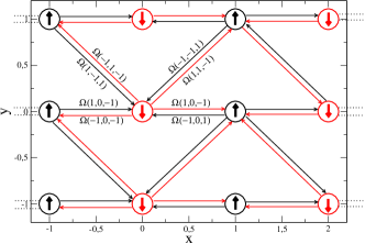
Figure 1: (Color online) A schematic of transition rates for the molecular motor corresponding to model (ii). Thick arrows indicate configurations with $\sigma$ up or down.

We illustrate the above results in two simplified systems: i) a chain of coupled non-linear oscillators with Hamiltonian $H=\frac{1}{2}\sum_{i=0}^{N}\left(mv_{i}^{2}+A_{1}\left(x_{i+1}-x_{i}\right)^{2}+\frac{2}{3}A_{2}\left(x_{i+1}-x_{i}\right)^{4}\right)$, with fixed boundary conditions $v_{0}=v_{N+1}=x_{0}=x_{N+1}=0$ where velocities evolve according to the Metropolis algorithm; ii) a model for a molecular motor driven by ATP hydrolysis introduced in Lau et al. (2007). In the latter model the evolution corresponds to an overdamped dynamics in two dimensions with transition rates for a jump $\delta x=0,\pm 1$ and $\delta y=0,\pm 1$, along the $x$ and $y$ direction respectively, given by $\Omega(\delta x,\delta y,\sigma)=\alpha\Theta(\delta x,\delta y,\sigma)e^{K\delta x\sigma+\frac{\varepsilon}{2}\sigma+\frac{\Delta\mu}{2}\Delta y}$. Here $\sigma=\pm 1$ indicates the states $b$ and $a$ of Lau et al. (2007), respectively, and $\Theta(\delta x,\delta y,\sigma)$ is a kinetic constraint that confines trajectories along the paths represented in Fig. 1. We set the parameter $\varepsilon$, corresponding to heat exchange by thermal activation, to zero and define $\delta x^{\prime}=\sigma\delta x$. This choice allows us to decouple the variables fluctuations, and in this case the evolution simply corresponds to discrete jumps in the $x^{\prime}-y$ plane, with kinetic constraints, under the action of an external force with components $\vec{f}=(K,\Delta\mu/2)$ and $\gamma=1$. As a consequence, Eq. (16) is still recovered by simply generalizing the above arguments to a two dimensional evolution.

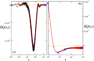
Figure 2: (Color online) The average heat exchange in (a) model (i) and (b) model (ii). Black circles are direct estimates obtained from Eq. (7) ($10^{7}$ data). The red continuous line is the estimate obtained by averaging Eq. (15). Blue crosses indicate the values of $t_{1}$ used in the next figure.

In Fig. 2 we plot the average value of the equal-time heat-exchange $\delta Q(t,t)$ for both models. In model (i) the temperature $T$, mass $m$, and $\zeta$ are fixed, time is measured in unit of Monte Carlo steps multiplied by $\zeta$ and energy is measured in units of the temperature $T$. We show results for a system with $N=32$, $T=100$, $m=10$, $\zeta=5\cdot 10^{-4}$, $A_{1}=800$ and $A_{2}=80$. In model (ii) we set $K=0.05$, $\Delta\mu=0.2$ and $\zeta_{\lambda}=1$ with initial position $x=0$, $y=0$ and $\sigma=-1$. Other parameters or initial conditions yield similar results. In both cases $\delta Q(t,t)$ is a non-monotonic function of time with both positive and negative values and relaxing to a the equilibrium value $\delta Q(t,t)=0$ for $t>t_{st}\simeq 5$ in model (i) and to a stationary asymptotic value $\delta Q_{\infty}$ smaller than zero in model (ii) with $t_{st}\simeq 200$. We wish to stress that Eq. (16) is verified for both models in the whole temporal range.

In the upper panels of Fig. 3 we plot $\delta Q(t_{1},t_{2})$ as function of $t_{2}-t_{1}$ for different values of $t_{1}$ corresponding to blue crosses in Fig 1. We observe that for model (i) (panel a) $\delta Q(t_{1},t_{2})$ is a non monotonic function with positive and negative values that converges to zero asymptotically ($t_{2}-t_{1}\gg 1$). Recalling the relationship between $\delta Q(t_{1},t_{2})$ and $T_{\textrm{eff}}$, this figure indicates that the effective temperature oscillates around the bath temperature $T$. The amplitude of the fluctutaions are controlled by the initial value of $\delta Q(t_{1},t_{1})$. In particular when $t_{1}>t_{st}$, equilibrium is reached and $\delta Q(t_{1},t_{2})=0$ in the whole temporal range. This is confirmed by the lower panel (panel c) where we plot the response function $R(t_{1},t_{2})$ versus the two-time correlation function $C(t_{1},t_{2})$ for different values of $t_{1}$. The equilibrium condition, corresponding to a straight line with slope $1$, is recovered for $t>t_{st}$. Furthermore, larger values of $|\delta Q(t_{1},t_{1})|$ also correspond to larger deviations from the equilibrium FDT. Also for model (ii) $\delta Q(t_{1},t_{2})$ presents both positive and negative values (Fig. 3b) with amplitudes controlled by the initial value $\delta Q(t_{1},t_{1})$. A fundamental difference between the two models can be observed at large times. Indeed, for $t_{2}-t_{1}\gg 1$, $\delta Q(t_{1},t_{2})$ converges to a $t_{1}$ independent asymptotic model $\delta Q_{\infty}<0$. In particular, for $t_{1}>t_{st}$ a costant heat-flux $\delta Q(t_{1},t_{2})$ is observed for all values of $t_{2}$ indicating a stationary non-equilibrium condition. This is confirmed by the parametric plot $TR$ vs $C$ (lower panel) indicating that curves reach a stationary asymptotic master curve, different from the equilibrium FDT, with $T_{\textrm{eff}}>T$.

Figure 3: (Color online) The upper panels show the generalized heat vs. time, calculated with Eq. (15) for (a) model (i) and (b) model (ii). The lower panels show the parametric plot of the response function vs. correlation function (both rescaled by $1/C(t_{1},t_{1})$) for (c) model (i) and (d) model (ii). The diagonal (black line) represents the equilibrium FDT in the form $TR=C$.

In conclusion, deriving a generalized Harada-Sasa formula (16) from a nonequilibrium FDT we have evidenced its validity for transient regimes and for systems evolving with jumps involving small entropy changes. This justifies the use of the HS relation in the framework of aging systems, as recently done with experimental results Gomez-Solano et al. (2012). Moreover, Eq. (16) includes two times rather than one, and can thus be used to define a generalized heat exchange and an effective temperature in terms of quantities that are experimentally accessible. It should be interesting to study the existence of similar relationships in processes with memory Deutsch and Narayan (2006); Maes et al. (2013), where the Markov hypothesis is violated, and in the presence of non-linear contributions in the external field Lippiello et al. (2008).

References

- Crisanti and Ritort (2003) A. Crisanti and F. Ritort, J. Phys. A 36, R181 (2003).
- Marini Bettolo Marconi et al. (2008) U. Marini Bettolo Marconi, A. Puglisi, L. Rondoni, and A. Vulpiani, Phys. Rep. 461, 111 (2008).
- Seifert and Speck (2010) U. Seifert and T. Speck, Europhys. Lett. 89, 10007 (2010).
- Baiesi and Maes (2013) M. Baiesi and C. Maes, New J. Phys. 15, 013004 (2013).
- Cugliandolo et al. (1997) L. F. Cugliandolo, J. Kurchan, and L. Peliti, Phys. Rev. E 55, 3898 (1997).
- Cugliandolo (2011) L. Cugliandolo, J. Phys. A 44, 483001 (2011).
- Harada and Sasa (2005) T. Harada and S. I. Sasa, Phys. Rev. Lett. 95, 130602 (2005).
- Harada and Sasa (2006) T. Harada and S. I. Sasa, Phys. Rev. E 73, 026131 (2006).
- Harada (2009) T. Harada, Phys. Rev. E 79, 030106(R) (2009).
- Deutsch and Narayan (2006) J. M. Deutsch and O. Narayan, Phys. Rev. E 74, 026112 (2006).
- Lander et al. (2012) B. Lander, J. Mehl, V. Blickle, C. Bechinger, and U. Seifert, Phys. Rev. E 86, 030401 (2012).
- Toyabe et al. (2007) S. Toyabe, H.-R. Jiang, T. Nakamura, Y. Murayama, and M. Sano, Phys. Rev. E 75, 011122 (2007).
- Toyabe et al. (2010) S. Toyabe, T. Okamoto, T. Watanabe-Nakayama, H. Taketani, S. Kudo, and E. Muneyuki, Phys. Rev. Lett. 104, 198103 (2010).
- Gomez-Solano et al. (2012) J. R. Gomez-Solano, A. Petrosyan, and S. Ciliberto, Europhys. Lett. 98, 10007 (2012).
- Cugliandolo et al. (1994) L. F. Cugliandolo, J. Kurchan, and G. Parisi, J. Phys. I France 4, 1641 (1994).
- Lippiello et al. (2005) E. Lippiello, F. Corberi, and M. Zannetti, Phys. Rev. E 71, 036104 (2005).
- Speck and Seifert (2006) T. Speck and U. Seifert, Europhys. Lett. 74, 391 (2006).
- Baiesi et al. (2009) M. Baiesi, C. Maes, and B. Wynants, Phys. Rev. Lett. 103, 010602 (2009).
- Gomez-Solano et al. (2009) J. R. Gomez-Solano, A. Petrosyan, S. Ciliberto, R. Chetrite, and K. Gawedzki, Phys. Rev. Lett. 103, 040601 (2009).
- Zamponi et al. (2005) F. Zamponi, F. Bonetto, L. F. Cugliandolo, and J. Kurchan, J. Stat. Mech. , P09013 (2005).
- Sekimoto (2010) K. Sekimoto, Stochastic Energetics (Springer-Verlag, Berlin, 2010).
- Lebowitz and Spohn (1999) J. L. Lebowitz and H. Spohn, J. Stat. Phys. 95, 333 (1999).
- Maes (1999) C. Maes, J. Stat. Phys. 95, 367 (1999).
- van Kampen (1961) N. van Kampen, Canad. J. Phys. 39, 551 (1961).
- Sarracino et al. (2010) A. Sarracino, D. Villamaina, G. Costantini, and A. Puglisi, J. Stat. Mech. , P04013 (2010).
- Lecomte et al. (2005) V. Lecomte, C. Appert-Rolland, and F. van Wijland, Phys. Rev. Lett. 95, 010601 (2005).
- Merolle et al. (2005) M. Merolle, J. P. Garrahan, and D. Chandler, Proc. Nat. Acad. Sci. USA 102, 10837 (2005).
- Maes and van Wieren (2006) C. Maes and M. H. van Wieren, Phys. Rev. Lett. 96, 240601 (2006).
- Note (1) In the original HS formula the correlation was computed for velocities after subtracting their steady state mean value, a step not necessary in our derivation.
- Note (2) To symmetrize at , one considers a contribution for before the transition and one following it. The correct form thus involves , which yields the correct Stratonovich convention for if the limit to diffusion processes is permormed.
- Lau et al. (2007) A. W. C. Lau, D. Lacoste, and K. Mallick, Phys. Rev. Lett. 99, 158102 (2007).
- Maes et al. (2013) C. Maes, S. Safaverdi, P. Visco, and F. van Wijland, Phys. Rev. E 87, 022125 (2013).
- Lippiello et al. (2008) E. Lippiello, F. Corberi, A. Sarracino, and M. Zannetti, Phys. Rev. E 78, 041120 (2008).