Friedel sum rule in the presence of topological defects for graphene

Baishali Chakraborty${}^{a},$    Kumar S. Gupta${}^{a},$    Siddhartha Sen${}^{b},$

^a Theory Division, Saha Institute of Nuclear Physics, 1/AF Bidhannagar, Calcutta 700064, India

^b CRANN, Trinity College Dublin, Dublin 2, Ireland

The Friedel sum rule is extended to deal with topological defects for the case of a graphene cone in the presence of an external Coulomb charge. The dependence in the way the number of states change due to both the topological defect as well as the Coulomb charge are studied. Our analysis addresses both the cases of a subcritical as well as a supercritical value of the Coulomb charge. We also discuss the experimental implications of introducing a self-adjoint extension of the system Hamiltonian. We argue that the boundary conditions following from the self-adjoint extension encode the effect of short range interactions present in the system.

1 Introduction

The Friedel sum rule provides a method for getting information about polarization charge due to an external charge impurity in the system[1, 2]. The screening charge around the impurity is directly proportional to the change in the number of states $\Delta N$ due to the Coulomb potential and Friedel sum rule shows that $\Delta N$ can be expressed in terms of a summation of scattering phase shifts at Fermi energy for all the angular momentum channels[3, 4, 5, 6, 7]. As $\Delta N$ is related to the LDOS of the system, the properties of the system which are related to LDOS can be obtained using this rule.

In this paper we analyze the Friedel sum rule in a gapless graphene cone in the presence of an external Coulomb charge[8]. The strength of the external Coulomb charge introduced in graphene can be classified as either subcritical or supercritical. The critical value of the Coulomb charge corresponds to a situation beyond which the system becomes quantum mechanically unstable[8, 9, 10, 11, 12, 13] and this leads to the 'fall to the centre'[10, 11] phenomenon. Graphene, experimentally fabricated in $2004$[14, 15, 16], provides an ideal laboratory to study this phenomenon. This is due to the fact that the Dirac type quasiparticles in graphene have a Fermi velocity which is approximately $300$ times smaller than the velocity of light. Thus the supercriticality is easily reached in graphene in presence of a relatively small external Coulomb charge impurity $Ze\sim 1$[9, 10, 11, 12, 13] and the atomic collapse[11] in this region leads to the formation of quasibound states. Recently such quasibound states have been observed experimentally[17] in gapless planer graphene. In this paper we study the supercritical Coulomb impurity in graphene in presence of a conical defect. The wavefunctions associated with the gapless Dirac type excitations in pristine graphene[18, 19, 20, 21, 22, 23, 24] pick up holonomy when the quasiparticles move around a closed path encircling a conical defect[25, 26, 27]. The holonomies due to topological defects[25, 26, 27, 28, 29, 30, 31, 32, 33, 34, 35, 36, 37, 38, 39, 40, 41, 42, 43, 44] can be realized by introducing a suitable flux tube passing through the origin[45, 46, 47, 48, 49, 50, 51]. We are thus lead to study the combined effect of the flux tube potential and the external Coulomb charge on graphene.

In addition to the supercritical region we analyze our system thoroughly for the subcritical values of the Coulomb charge. In the subcritical region for a certain range of system parameters we found that a single real parameter is required for labeling the boundary conditions at the location of the defects. To understand the physical origin of such a parameter we recall that the Coulomb charge as well as the conical defect can give rise to short range interactions in graphene. Such interactions cannot be directly incorporated in the Dirac equation as the latter is valid only in the low energy or long-wavelength limit. However the combined effect of such short range interactions can be encoded in the boundary conditions[52, 53, 54, 55] by the parameter. This additional real parameter ensures current conservation leading to a self-adjoint Hamiltonian and unitary evolution of the quantum system[56, 57, 58]. We show that the scattering phase shift and consequently $\Delta N$ depend explicitly on this parameter labeling the boundary conditions in the graphene cone. This parameter is determined empirically as it cannot be obtained by theory.

This paper is organized as follows. In the next Section we set up the Friedel sum rule for gapless graphene cone with a point charge at the apex. Then the analysis of the spectrum is done in the subcritical region, where we obtain the scattering phase shifts and change in the number of states and show how these physical quantities depend explicitly on the sample topology. After that we discuss the effect of generalized boundary conditions on the spectrum. In the next section the analysis of the corresponding spectrum is done in the supercritical region. We end this paper with some discussion and outlook.

2 Friedel Sum Rule for massless graphene cone

The low energy properties of the quasiparticles near a Dirac point in a planer gapless graphene sample[18, 19, 20, 21, 22, 23, 24] in the presence of an external Coulomb charge is given by

$$\left[-i\hbar v_{F}(\sigma_{1}\partial_{x}+\sigma_{2}\partial_{y})+\sigma_{0}\left(\frac{-\alpha}{r}\right)\right]\Psi=E\Psi,$$ (1)

where $r$ is the radial coordinate in the two-dimensional $x-y$ plane and $\alpha$ is the Coulomb interaction strength. The Pauli matrices $\sigma_{1,2,3}$ and the identity matrix $\sigma_{0}$ act on the pseudospin indices $A,B$.

When a conical defect is introduced in graphene by removing $n$ number of sectors subtending an angle $\frac{2n\pi}{6}$ at the centre and the edges of the removed sector are identified, the angular boundary condition obeyed by the Dirac spinor is modified. Due to the identification of the two edges of the removed sector the frame $\{\hat{e}_{x},\hat{e}_{y}\}$ becomes discontinuous across the joining line. Therefore we choose a new set of frames which is rotated with respect to the old frame $(\hat{e}_{x},\hat{e}_{y})$ by an angle $\omega=\theta+\frac{\pi}{2}$ [8]. The effect of the conical topology can be equivalently described by introducing a magnetic flux tube passing through the centre of the plane graphene sheet. The magnetic vector potential associated with the flux tube replaces the ordinary derivatives in the Hamiltonian by the corresponding covariant derivatives . Therefore the Dirac equation for massless graphene cone becomes

$$H\Psi_{\nu}=E_{\nu}\Psi_{\nu},$$ (2)

where

$$H=\left(\begin{array}[]{cc}-\frac{\alpha}{r}&\partial_{r}-\frac{i}{r(1-\frac{n}{6})}\partial_{\theta}\pm\frac{\frac{n}{4}}{r(1-\frac{n}{6})}+\frac{1}{2r}\\ -\partial_{r}-\frac{i}{r(1-\frac{n}{6})}\partial_{\theta}\pm\frac{\frac{n}{4}}{r(1-\frac{n}{6})}-\frac{1}{2r}&-\frac{\alpha}{r}\end{array}\right).$$ (5)

For the wave function $\Psi_{\nu}$ we use the following ansatz.

$$\Psi_{\nu}=\sum_{j}\left(\begin{array}[]{c}\Psi_{A\nu}^{(j)}(r)\\ \Psi_{B\nu}^{(j)}(r)\end{array}\right)e^{ij\theta},$$ (8)

where $j$ is the total angular momentum quantum number. The radial Dirac equation in each angular momentum channel $j$ is given by

$$\left(\begin{array}[]{cc}E_{\nu}+\frac{\alpha}{r}&-\{\partial_{r}+(\lambda+\frac{1}{2})\frac{1}{r}\}\\ \{\partial_{r}-(\lambda-\frac{1}{2})\frac{1}{r}\}&E_{\nu}+\frac{\alpha}{r}\end{array}\right)\left(\begin{array}[]{c}\Psi_{A\nu}^{(j)}(r)\\ \Psi_{B\nu}^{(j)}(r)\end{array}\right)=0,$$ (13)

where $\lambda=\frac{j\pm\frac{n}{4}}{1-\frac{n}{6}}$. In the absence of the external Coulomb potential the equations for the components of $\Psi_{\nu}^{j}(r)$ can be decoupled into Bessel equations. The equation for the Dirac spinor component $\Psi_{A\nu}^{j}(r)$ is given by

$$\frac{d^{2}}{dr^{2}}\Psi_{A\nu}+\frac{1}{r}\frac{d}{dr}\Psi_{A\nu}+\left[E_{\nu}^{2}-\frac{(\lambda-\frac{1}{2})^{2}}{r^{2}}\right]\Psi_{A\nu}=0$$ (14)

and the solution regular at the origin is

$$\Psi_{A\nu}^{j}(r)=C(E_{\nu})J_{\lambda-\frac{1}{2}}(E_{\nu}r).$$ (15)

Using a suitable normalization condition we get the expression for $C(E_{\nu})$ to be $\sqrt{\frac{E_{\nu}}{2}}$ . From $\Psi_{A\nu}$ the expression for $\Psi_{B\nu}$ can be obtained with the help of Eq.(13). When $r\rightarrow\infty$, the asymptotic expression for $\Psi_{A\nu}$ is given by

$$\Psi_{A\nu}^{j}(r)\rightarrow\frac{1}{\sqrt{\pi r}}\mbox{cos}\left(E_{\nu}r-\frac{\lambda\pi}{2}\right).$$ (16)

Substituting this expression in Eq. (13) we get,

$$\lim_{r\rightarrow\infty}\Psi_{B\nu}^{j}(r)\rightarrow\frac{1}{\sqrt{\pi r}}\mbox{sin}\left(E_{\nu}r-\frac{\lambda\pi}{2}\right).$$ (17)

To evaluate the total change in the number of states $\Delta N$ around the Coulomb charge at the apex of the massless graphene cone, now we consider a two dimensional circular area of a large radius $R$. This area has the Coulomb charge at its centre. The magnetic flux tube representing the nontrivial holonomies produced by the conical defect also passes through the centre. The asymptotic behaviors of the wave function will be used for the evaluation process. We proceed with multiplying Eq. (2) by the adjoint of the Dirac spinor and the adjoint of Eq. (2) by the Dirac spinor.

The adjoint of Eq.(2) is given by

$$(H\Psi_{\nu})^{\dagger}=E_{\nu}\Psi_{\nu}^{\dagger}.$$ (18)

Multiplying Eq.(18) by $\Psi_{\nu^{\prime}}$ and Eq. (2) for $\Psi_{\nu^{\prime}}$ by $\Psi_{\nu}^{\dagger}$ and subtracting we obtain the following .

$$(E_{\nu^{\prime}}-E_{\nu})\Psi_{\nu}^{\dagger}\Psi_{\nu^{\prime}}=[-i\vec{\nabla}\cdotp\{\Psi_{\nu}^{\dagger}\vec{\sigma}\Psi_{\nu^{\prime}}\}]+\frac{i}{r}\{\Psi_{\nu}^{\dagger}\sigma_{2}\Psi_{\nu^{\prime}}\}.$$ (19)

Now integrating Eq.(19) over the whole area we have

$$(E_{\nu^{\prime}}-E_{\nu})\iint d^{2}r\Psi_{\nu}^{\dagger}\Psi_{\nu^{\prime}}=\iint d^{2}r[-i\vec{\nabla}\cdotp\{\Psi_{\nu}^{\dagger}\vec{\sigma}\Psi_{\nu^{\prime}}\}]+\iint d^{2}r\frac{i}{r}\{\Psi_{\nu}^{\dagger}\sigma_{2}\Psi_{\nu^{\prime}}\}.$$ (20)

Application of divergence theorem gives

$$\iint d^{2}r\Psi_{\nu}^{\dagger}\Psi_{\nu^{\prime}}=\frac{R}{(E_{\nu^{\prime}}-E_{\nu})}\oint d\theta(-i)\{\Psi_{\nu}^{\dagger}(\vec{\sigma}\cdotp\hat{r})\Psi_{\nu^{\prime}}\}+\iint\frac{d^{2}r}{(E_{\nu^{\prime}}-E_{\nu})}\frac{i}{r}\{\Psi_{\nu}^{\dagger}\sigma_{2}\Psi_{\nu^{\prime}}\}.$$ (21)

At large distance, the second term on the R.H.S. of Eq. (21) gives negligible contribution. Therefore the above integral can be expanded as

$$\iint d^{2}r\Psi_{\nu}^{\dagger}\Psi_{\nu^{\prime}}=\frac{2\pi R}{(E_{\nu^{\prime}}-E_{\nu})}\sum_{j}[\Psi_{A\nu}^{j*}(r)\Psi_{B\nu^{\prime}}^{j}(r)-\Psi_{B\nu}^{j*}(r)\Psi_{A\nu^{\prime}}^{j}(r)].$$ (22)

Eq. (22) gives the local density of states at a particular energy level $E_{\nu}$. So the total change in the number of states around the Coulomb potential can be found by integrating the expression up to the Fermi energy level $E_{F}$ in the presence and in the absence of the external Coulomb potential and then by obtaining the difference between the two integrals.

$$\Delta N=\lim_{r\longrightarrow\infty}\lim_{E_{\nu^{\prime}}\longrightarrow E_{\nu}}\int_{0}^{E_{F}}dE_{\nu}\iint d^{2}r[\Psi_{\nu}^{\dagger}\Psi_{\nu^{\prime}}-\Psi_{\nu 0}^{\dagger}\Psi_{\nu^{\prime}0}].$$ (23)

Here $\Psi_{\nu 0}$ represents the Dirac spinor of the massless graphene cone in the absence of the external Coulomb potential. Now putting the asymptotic expression of the wave function in Eq. (23) we can obtain the Friedel sum rule for massless graphene cone [5]. According to the rule

$$\Delta N=\frac{1}{\pi}\sum_{j}[\delta_{j}(E_{F})-\delta_{j}(0)].$$ (24)

Here $\delta_{j}$ represents the scattering phase shift in the $j$-th angular momentum channel. As the scattering phase shift contains the term $\lambda$ both for the subcritical and supercritical region, the Friedel sum rule depends explicitly on the topological defect of the system.

This rule can also be established by calculating directly the DOS using the Green function $G_{\alpha}(\mathbf{r_{1}},\mathbf{r_{2}},E+i\epsilon)$ [6, 7] and applying the formula

$$\rho_{\alpha}(E)=-\frac{1}{\pi}\mbox{Im Tr}G_{\alpha}(\mathbf{r_{1}},\mathbf{r_{2}},E+i\epsilon).$$ (25)

The Green function can be expanded in terms of the eigenfunctions $\Psi_{\nu}(\mathbf{r},\theta)$ in polar coordinates. Using the eigenfunctions in the presence and in the absence of the Coulomb potential the change in DOS can be calculated. The change in the number of states can then be obtained by

$$\Delta N=\int_{-\infty}^{E_{F}}dE^{\prime}[\rho_{\alpha}(E^{\prime})-\rho_{0}(E^{\prime})].$$ (26)

Putting the expressions of the eigenfunctions in the Green function we can find out that the change in number of states depends on the sum of the scattering phase shifts over all the angular momentum channels.

We shall analyse the effect of conical topology on the Friedel sum rule for massless graphene for both the subcritical and supercritical region in the following two sections.

3 Subcritical region

In this section we shall obtain the expression of scattering phase shift for the massless graphene with a conical defect in presence of a subcritical Coulomb charge. To solve the Dirac equation Eq. (2) in presence of a subcritical Coulomb charge we assume

$$\Psi_{\nu}(r,\theta)=\sum_{j}\left(\begin{array}[]{c}\Psi_{A\nu}^{(j)}(r)\\ i\Psi_{B\nu}^{(j)}(r)\end{array}\right)e^{-iE_{\nu}r}{r}^{\beta-(1/2)}e^{ij\theta},$$ (29)

where $\beta=\sqrt{\lambda^{2}-\alpha^{2}}$ and we use two new functions $u_{\nu}^{(j)}(r)$ and $v_{\nu}^{(j)}(r)$ defined by $\Psi_{A\nu}^{(j)}(r)=v_{\nu}^{(j)}(r)+u_{\nu}^{(j)}(r),~{}\Psi_{B\nu}^{(j)}(r)=v_{\nu}^{(j)}(r)-u_{\nu}^{(j)}(r)$ to get the following equations.

$$r\frac{dv_{\nu}^{(j)}(r)}{dr}+(\beta+i\alpha)v_{\nu}^{(j)}(r)-\lambda u_{\nu}^{(j)}(r)=0~{}~{}~{}~{}~{}~{}~{}~{}~{}$$ (30)

and

$$r\frac{du_{\nu}^{(j)}(r)}{dr}+(\beta-i\alpha-2iE_{\nu}r)u_{\nu}^{(j)}(r)-\lambda v_{\nu}^{(j)}(r)=0.~{}~{}~{}~{}~{}~{}~{}~{}~{}$$ (31)

Combining Eqs. (30) and (31) we get

$$s\frac{d^{2}v^{(j)}(s)}{ds^{2}}+(1+2\beta-s)\frac{dv^{(j)}(s)}{ds}-\left(\beta+i\alpha\right)v^{(j)}(s)=0,$$ (32)

where $s=-2ikr$, with $k=-E_{\nu}$.

The solution of Eq. (32) which is regular at the origin is given by

$$v^{(j)}(s)=AM\left(\beta+i\alpha,~{}1+2\beta,~{}s\right),$$ (33)

where $M$ is the confluent hypergeometric function[59] and $A$ is a constant which depends on the energy of the system.

Substituting this expression of $v^{(j)}(s)$ from Eq.(33) in Eq.(30) we have

$$u^{(j)}(s)=A\frac{(\beta+i\alpha)}{\lambda}M\left(1+\beta+i\alpha,~{}1+2\beta,~{}s\right).$$ (34)

Using the asymptotic form of $v^{(j)}(s)$ and $u^{(j)}(s)$ we can find out the expression of the scattering phase shift to be

$$\delta_{j}(k)=-\alpha\ln(2kr)+\arg[\Gamma(1+\beta+i\alpha)]-\frac{\pi\beta}{2}-\frac{1}{2}\tan^{-1}\left(\frac{\alpha}{\beta}\right)+\left|\frac{\lambda\pi}{2}\right|.$$ (35)

With the help of this expression and the Friedel sum rule we have found out the dependence of $\Delta N$ on the Coulomb potential and the conical defect in massless graphene. We have plotted the dependence in Fig.(1). The change in the number of states is directly proportional to the polarization charge induced in the system by the external Coulomb charge. Therefore from Fig.(1) we can determine the dependence of polarization charge on subcritical Coulomb potential using Friedel sum rule.

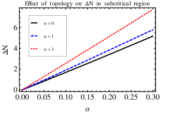
Figure 1: Dependence of change in the number of states on subcritical Coulomb potential using Friedel sum rule.

From the plot we can see that for different values of $n$ i.e. for different topology the polarization charge increases with the subcritical Coulomb potential at a different rate. It indicates that the change in the number of states around the external subcritical Coulomb charge depends on the topology of the system and with the increase in the angular deficit of the cone the rate of this change increases.

3.1 Generalized boundary conditions

The conical defect and the Coulomb charge impurity can give rise to some short range interactions in the graphene system. These interactions cannot be included as dynamical terms in the Dirac equation as the latter is valid for only low energy and long wavelength excitations. However, through the choice of suitable boundary conditions prescribed by von Neumann for systems with unitary time evolution and probability current conservation[56, 57, 58], combined effect of those interactions can be considered which is discussed below[52, 53, 54, 55].

The Dirac operator $H$ in Eq.(2) has an angular part and a radial part. The angular boundary condition is kept unchanged as the angular part operates on a domain spanned by the antiperiodic functions $e^{ij\theta}$ where $j$ is a half integer. The radial Dirac operator $H_{r}$ is given by

$$H_{r}=\left(\begin{array}[]{cc}-\frac{\alpha}{r}&\{\partial_{r}+(\lambda+\frac{1}{2})\frac{1}{r}\}\\ -\{\partial_{r}-(\lambda-\frac{1}{2})\frac{1}{r}\}&-\frac{\alpha}{r}\end{array}\right).$$ (38)

It is symmetric in the domain $\mathcal{D}_{0}=C_{0}^{\infty}(R^{+})$ consisting of infinitely differentiable functions of compact support in the real half line $R^{+}$ and its adjoint operator $H_{r}^{\dagger}$ has the same expression as $H_{r}$ but its domain can be different. The domain of self-adjointness of the operator $H_{r}$ can be determined by using the equation

$$H_{r}^{\dagger}\Psi_{\pm}=\pm\frac{i}{l}\Psi_{\pm},$$ (39)

where $l$ has the dimension of length and

$$\Psi_{\pm}(r)=\sum_{j}\left(\begin{array}[]{c}v_{\pm}^{(j)}(r)+u_{\pm}^{(j)}(r)\\ i(v_{\pm}^{(j)}(r)-u_{\pm}^{(j)}(r))\end{array}\right)e^{\pm\frac{r}{l}}r^{\beta-\frac{1}{2}}.$$ (42)

The total number of square integrable, linearly independent solutions of Equation(39) gives the deficiency indices for $H_{r}$ and they are denoted by $n_{\pm}$. The existence of imaginary eigenvalues $\pm\frac{i}{l}$ in the spectrum is a measure of the deviation of the operator $H_{r}$ from self-adjointness. The non zero deficiency indices serve as the measurement of this deviation. The deficiency indices classify $H_{r}$ in three different ways [52] : $(1)$ When $n_{+}=n_{-}=0$, $H_{r}$ is essentially self-adjoint in $\mathcal{D}_{0}(H_{\rho})$. $(2)$ When $n_{+}=n_{-}\neq 0$, $H_{r}$ is not self-adjoint in $\mathcal{D}_{0}(H_{\rho})$ but it can admit self-adjoint extensions. $(3)$ When $n_{+}\neq n_{-}$, $H_{r}$ cannot have self-adjoint extensions.

Eq. (39) leads to the following two coupled differential equations:

$$r\frac{dv_{\pm}^{(j)}(r)}{dr}+(\beta+i\alpha)v_{\pm}^{(j)}(r)-\lambda u_{\pm}^{(j)}(r)=0~{}~{}~{}~{}~{}~{}~{}~{}~{}$$ (43)

and

$$r\frac{du_{\pm}^{(j)}(r)}{dr}+(\beta-i\alpha\pm\frac{2r}{l})u_{\pm}^{(j)}(r)-\lambda v_{\pm}^{(j)}(r)=0.~{}~{}~{}~{}~{}~{}~{}~{}~{}$$ (44)

Combining Eqs. (43) and (44) we get

$$s\frac{d^{2}v_{\pm}^{(j)}(s)}{ds^{2}}+(1+2\beta-s)\frac{dv_{\pm}^{(j)}(s)}{ds}-\left(\beta+i\alpha\right)v_{\pm}^{(j)}(s)=0,$$ (45)

where $s=\mp\frac{2r}{l}$ for $E=\pm\frac{i}{l}$.

In order to solve Eq. (45) let us first consider the case where $s=-\frac{2r}{l}$ i.e. $E=\frac{i}{l}$. The solution can be written as

$$v_{+}=e^{-\frac{2r}{l}}U\left(1+\beta-i\alpha,1+2\beta,\frac{2r}{l}\right).$$ (46)

Putting this expression for $v_{+}$ in Eq. (43) we obtain

$$u_{+}=-\frac{e^{-\frac{2r}{l}}}{\lambda}U\left(\beta-i\alpha,1+2\beta,\frac{2r}{l}\right).$$ (47)

Therefore the radial part of the upper component of the wave function becomes

$$\Psi_{A+}=e^{-\frac{r}{l}}\left[U\left(1+\beta-i\alpha,1+2\beta,\frac{2r}{l}\right)-\frac{1}{\lambda}U\left(\beta-i\alpha,1+2\beta,\frac{2r}{l}\right)\right]r^{\beta-\frac{1}{2}}.$$ (48)

This component $\Psi_{A+}$ spans the $E=+\frac{i}{l}$ deficiency subspace. In order to find conditions under which $\Psi_{A+}$ and consequently $\Psi_{+}$ has square integrable solutions, we notice that as $r\rightarrow\infty,~{}\Psi_{A+}\rightarrow 0$. As a result we can say $\Psi_{A+}$ is square integrable at infinity. When $r\rightarrow 0$,

$$\int|\Psi_{A+}|^{2}rdr\sim\int r^{-2\beta}dr+\mbox{converging terms}.$$ (49)

Therefore we can say that $\Psi_{A+}$ is a square integrable function for the range $0<\beta<\frac{1}{2}$. Proceeding in the similar manner we can show that for the specified range of $\beta$ the entire radial wave function is square integrable and the deficiency index $n_{+}=1$ for a graphene cone in presence of an external Coulomb charge.

Next we consider the case where $s=\frac{2r}{l}$ i.e. $E=-\frac{i}{l}$. In this case the solution can be written as

$$v_{-}=U\left(\beta+i\alpha,1+2\beta,\frac{2r}{l}\right).$$ (50)

Putting this expression for $v_{-}$ again in Eq. (43) we obtain

$$u_{-}=\frac{(\beta+i\alpha)(-\beta+i\alpha)}{\lambda}U\left(1+\beta+i\alpha,1+2\beta,\frac{2r}{l}\right).$$ (51)

Therefore we have

$$\Psi_{A-}=e^{-\frac{r}{l}}\left[U\left(\beta+i\alpha,1+2\beta,\frac{2r}{l}\right)+\frac{(\beta+i\alpha)(-\beta+i\alpha)}{\lambda}U\left(1+\beta+i\alpha,1+2\beta,\frac{2r}{l}\right)\right]r^{\beta-\frac{1}{2}}.$$ (52)

as the radial part of the upper component of the wave function which spans the $E=-\frac{i}{l}$ deficiency subspace. Analysing as before, we notice that when $0<\beta<\frac{1}{2}$, for $E=-\frac{i}{l}$ also we have a single square integrable solution for the wave-function indicating $n_{-}=1$.

As the deficiency indices $n_{+}=n_{-}=1$, following von Neumann’s analysis we can say that the radial Hamiltonian $H_{r}$ admits a one parameter family of self-adjoint extension in this case. The domain representing the boundary conditions for which $H_{r}$ is self-adjoint is given by ${\mathcal{D}}_{\Phi}(H_{r})={\mathcal{D}}_{0}(H_{r})\oplus\{e^{i\frac{\Phi}{2}}{\Psi}_{+}+e^{-i\frac{\Phi}{2}}{\Psi}_{-}\},$ where $\Phi\in R~{}\mbox{mod}~{}2\pi$ is the self-adjoint extension parameter.

Using the properties of the confluent hypergeometric functions, at $r\rightarrow 0$ we have,

$$\Psi_{A_{+}}=\frac{\pi}{\lambda\sin\pi(1+2\beta)}\left[\frac{(\lambda+\beta+i\alpha)}{\Gamma(1-\beta-i\alpha)\Gamma(1+2\beta)}r^{\beta-\frac{1}{2}}-\left(\frac{2}{l}\right)^{-2\beta}\frac{(\lambda-\beta+i\alpha)}{\Gamma(1+\beta-i\alpha)\Gamma(1-2\beta)}r^{-\beta-\frac{1}{2}}\right]$$ (53)

and

$$\Psi_{A_{-}}=\frac{\pi}{\lambda\sin\pi(1+2\beta)}\left[\frac{(\lambda+\beta+i\alpha)}{\Gamma(-\beta+i\alpha)\Gamma(1+2\beta)}r^{\beta-\frac{1}{2}}-\left(\frac{2}{l}\right)^{-2\beta}\frac{(\lambda-\beta+i\alpha)}{\Gamma(\beta+i\alpha)\Gamma(1-2\beta)}r^{-\beta-\frac{1}{2}}\right].$$ (54)

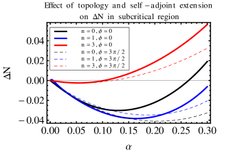
Figure 2: Dependence of $\Delta N$ on subcritical Coulomb potential using Friedel sum rule and generalized boundary condition. The solid lines correspond to $\Phi=0$ and the dashed lines correspond to $\Phi=\frac{3\pi}{2}$.

To find out the scattering phase shift using the generalized boundary conditions, we first try to obtain the solution of Eq.(32) which gives the physical scattering states. The required solution is

$$v(s)=C_{1}M\left(\beta+i\alpha,~{}1+2\beta,~{}s\right)+C_{2}s^{-2\beta}M\left(-\beta+i\alpha,~{}1-2\beta,~{}s\right),$$ (55)

where $s=-2ikr$.

Now with the help of Eq.(30) we have

$$u(s)=C_{1}\frac{(\beta+i\alpha)}{\lambda}M\left(1+\beta+i\alpha,~{}1+2\beta,~{}s\right)+C_{2}s^{-2\beta}\frac{(-\beta+i\alpha)}{\lambda}M\left(1-\beta+i\alpha,~{}1-2\beta,~{}s\right).$$ (56)

Using Eq.(55) and Eq.(56) we get the upper component of the wave-function $\Psi$ as

$$\Psi_{A}(s) = r^{\beta-\frac{1}{2}}e^{ikr}\{C_{1}\frac{(\beta+i\alpha)}{\lambda}M\left(1+\beta+i\alpha,~{}1+2\beta,~{}s\right)$$ (57)

$$+ C_{2}s^{-2\beta}\frac{(-\beta+i\alpha)}{\lambda}M\left(1-\beta+i\alpha,~{}1-2\beta,~{}s\right)+C_{1}M\left(\beta+i\alpha,~{}1+2\beta,~{}s\right)$$

$$+ C_{2}s^{-2\beta}M\left(-\beta+i\alpha,~{}1-2\beta,~{}s\right)\}.$$

In the limit $r\rightarrow 0$ we match the behaviour of this physical wave function with a typical element of ${\mathcal{D}}_{\Phi}(H_{r})$ to ensure the unitary evolution of $H_{r}$. When $r\rightarrow 0$, Eq.(57) gives

$$\Psi_{A}(r)=C_{1}\frac{\lambda+\beta+i\alpha}{\lambda}r^{\beta-\frac{1}{2}}+C_{2}\frac{(\lambda-\beta+i\alpha)}{\lambda}(-2ik)^{-2\beta}r^{-\beta-\frac{1}{2}}.$$ (58)

In the same limit a typical element of the domain ${\mathcal{D}}_{\Phi}(H_{r})$ is given by

$$\Psi(r)=\eta(e^{\frac{i\Phi}{2}}\Psi_{+}+e^{\frac{-i\Phi}{2}}\Psi_{-}).$$ (59)

Comparing Eq.(58) and Eq.(59) we have

$$C_{1}=\frac{\eta\pi}{\sin\pi(1+2\beta)}\left[\frac{e^{\frac{i\Phi}{2}}}{\Gamma(1-\beta-i\alpha)\Gamma(1+2\beta)}+\frac{e^{\frac{-i\Phi}{2}}}{\Gamma(-\beta+i\alpha)\Gamma(1+2\beta)}\right]$$ (60)

and

$$C_{2}=-(-ikl)^{2\beta}\frac{\eta\pi}{\sin\pi(1+2\beta)}\left[\frac{e^{\frac{i\Phi}{2}}}{\Gamma(1+\beta-i\alpha)\Gamma(1-2\beta)}+\frac{e^{\frac{-i\Phi}{2}}}{\Gamma(\beta+i\alpha)\Gamma(1-2\beta)}\right].$$ (61)

Now to find the scattering matrix and the phase shift we investigate the asymptotic behaviour of the wave-function $\Psi$ with the help of the properties of the confluent hypergeometric functions. When $r\rightarrow\infty$ we note that

$$\Psi_{A}(r)= \!\!\!\!\!\!\!\!\!\!(-2ik)^{-\beta}(-i)^{i\alpha}\left[C_{1}\frac{\beta+i\alpha}{\lambda}\frac{\Gamma(1+2\beta)}{\Gamma(1+\beta+i\alpha)}+C_{2}\frac{-\beta+i\alpha}{\lambda}\frac{\Gamma(1-2\beta)}{\Gamma(1-\beta+i\alpha)}\right]\frac{e^{-i[kr-\alpha\ln(2kr)]}}{\sqrt{r}}$$

$$\!\!\!\!\!\!\!\!\!\!\!\!\!\!\!\!\!\!+\ (-2ik)^{-\beta}(-i)^{-i\alpha}\left[C_{1}\frac{\Gamma(1+2\beta)}{\Gamma(1+\beta-i\alpha)}e^{-i\pi(\beta+i\alpha)}+C_{2}\frac{\Gamma(1-2\beta)}{\Gamma(1-\beta-i\alpha)}e^{-i\pi(-\beta+i\alpha)}\right]\frac{e^{i[kr-\alpha\ln(2kr)]}}{\sqrt{r}}.$$

The scattering matrix $S$ and the corresponding phase shift $\delta(k)$ is given by

$$S=e^{2i\delta(k)}=-\lambda e^{-2i\alpha\ln(2kr)}\left[\frac{F+G}{\lambda^{2}F^{*}+G^{*}}\right],$$ (63)

where

$$F=\left\{\frac{e^{-\frac{i\pi\beta}{2}}-(kl)^{2\beta}e^{\frac{i\pi\beta}{2}}}{\Gamma(1+\beta-i\alpha)\Gamma(1-\beta-i\alpha)}\right\}e^{\frac{i\Phi}{2}}$$ (64)

and

$$G=-\beta\left\{\frac{e^{-\frac{i\pi\beta}{2}}}{\Gamma(1+\beta-i\alpha)\Gamma(1-\beta+i\alpha)}+\frac{(kl)^{2\beta}e^{\frac{i\pi\beta}{2}}}{\Gamma(1-\beta-i\alpha)\Gamma(1+\beta+i\alpha)}\right\}e^{-\frac{i\Phi}{2}}.$$ (65)

From Eq.(63) we can see that the scattering matrix and the phase shift explicitly depend on the self-adjoint extension parameter $\Phi$ or equivalently the generalized boundary conditions. We should always keep in mind that the conditions are valid only for the range $0<\beta<\frac{1}{2}$. Different values of $\Phi$ corresponds to different combinations of the short range interactions induced by the external Coulomb charge which gives rise to inequivalent quantum description of the gapless graphene cone. The value of $\Phi$ cannot be determined analytically but by measuring quantities depending on the scattering data, it can be fixed empirically.

The dependence of the change in the number of states on the Coulomb potential around the Coulomb charge can be determined with the help of the Friedel sum rule, which connects the scattering phase shifts with the change in the number of states. Therefore using Eq.(63) we plot the dependence of the change in the number of states on Coulomb potential for the parameter range $0<\beta<\frac{1}{2}$ for different values of $\Phi$. From the plot we can clearly see that $\Delta N$ depends on the topology of the system as well as the boundary condition applied on it.

4 supercritical region

In this section for any given value of $n$ and $j$, we always choose $\alpha$ greater than the corresponding value of $|\lambda|$ to ensure that the coupling is in the supercritical region. We define $\beta$ as $i\eta$ where $\eta=\sqrt{\alpha^{2}-\lambda^{2}}$. Then the solution of Eq. (32) is given by

$$v^{(j)}(s)=C_{1}M\left(i(\eta+\alpha),~{}1+2i\eta,~{}s\right)+C_{2}{s}^{-2i\eta}M\left(i(\alpha-\eta),~{}1-2i\eta,~{}s\right).$$ (66)

From Eqs. (30) and (32) we get

$$u^{(j)}(s)=-iC_{1}\chi M\left(1+i(\eta+\alpha),~{}1+2i\eta,~{}s\right)-i(C_{2}/\chi){s}^{-2i\eta}M\left(1+i(\alpha-\eta),~{}1-2i\eta,~{}s\right),$$ (67)

where $\chi=\sqrt{\frac{\alpha+\eta}{\alpha-\eta}}$.

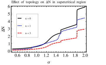
Figure 3: Dependence of change in the number of states on supercritical Coulomb potential using Friedel sum rule.

In order to proceed, we use the zigzag edge boundary condition $[u^{(j)}(l_{0})-v^{(j)}(l_{0})]=0$, where $l_{0}$ is a distance from the apex, of the order of the lattice scale in graphene. This gives

$$C_{2}=e^{2i\xi(k)}\chi e^{\pi\eta}C_{1}~{}~{}~{}~{}~{}~{}\mbox{where}~{}~{}~{}~{}~{}e^{2i\xi(k)}=\frac{i(1+i\chi)}{(1-i\chi)}e^{2i\eta\mbox{ln}(2kl_{0})}.$$ (68)

From the above, we obtain the scattering matrix $S$ as

$$S=e^{2i\delta_{j}(k)}=\left[\frac{h_{\alpha,\eta}+e^{2i\xi(k)}e^{-\pi\eta}\chi h_{\alpha,-\eta}}{e^{\pi\eta}\chi h^{*}_{\alpha,-\eta}+e^{2i\xi(k)}h^{*}_{\alpha,\eta}}\right]e^{-2i\alpha\mbox{ln}(2kr)},$$ (69)

where $h_{\alpha,\eta}=\frac{\Gamma(1+2i\eta)}{\Gamma(1+i\eta-i\alpha)}$.

From Eq. (69) we obtain the scattering phase as

$$\delta_{j}(k)=\mbox{arg}[e^{-i\xi(k)}+ce^{i\xi(k)}]-\alpha\mbox{ln}(2kr)+\mbox{arg}(h_{\alpha,\eta}),$$ (70)

where $c=e^{-\pi\eta}\chi\frac{h_{\alpha,-\eta}}{h_{\alpha,\eta}}$.

From Eq.(70) we can see that the second term $-\alpha\mbox{ln}(2kr)$ in the R.H.S. is also present in the subcritical region. It is typical for a phase coming from the Coulomb tail and does not affect the polarization at a finite distance[10]. In addition to that term the scattering phase shift in the supercritical region has a strong energy dependence through the first term in the R.H.S. of Eq.(70). Keeping in mind the relation between polarization charge and change in the number of states we can find out the dependence of the polarization charge on the supercritical Coulomb potential from the scattering phase shift at Fermi energy according to the Friedel sum rule using Eq.(70).

Though the nature of dependence of $\Delta N$ on supercritical Coulomb potential is quite different from that of the subcritical region, here also we can see that for different values of $n$, $\Delta N$ increases with the supercritical Coulomb potential in a different manner. The sharp increase in $\Delta N$ at certain values of $\alpha$ corresponds to the quasibound states formed in this region. The plot shows that the rate of change in the number of states around the external supercritical Coulomb charge changes with the angular deficit of the graphene cone.

5 Conclusion

In this paper we have studied the Friedel sum rule for graphene with a conical defect in presence of an external Coulomb charge. The eigenstates of the Dirac equation valid for the low energy excitations in graphene cone[8] have been used to obtain the relation between the change in the number of states $\Delta N$ due to the Coulomb impurity and the summation of the scattering phase shifts at Fermi energy in different angular momentum channels. As the scattering phase shifts explicitly depend on the topology of the graphene cone, we have shown $\Delta N$ will also depend on the angle of the cone.

We have plotted the dependence of $\Delta N$ on Coulomb potential using the Friedel sum rule for both subcritical and supercritical values of the Coulomb impurity. In the subcritical region from Fig.1 we can see that $\Delta N$ increases with the increase in the value of $n$ for a certain value of $\alpha$. As polarization charge is directly proportional to $\Delta N$, we can say that for a fixed value of external subcritical Coulomb charge, polarization charge increases with the decrease in opening angle of the graphene cone. The conical defect and the external charge impurity can lead to short range interactions in graphene. Those interactions cannot be directly included in the Dirac equation because the latter is valid only in the long wavelength limit[52, 53, 54, 55]. The single real parameter which labels the boundary conditions can be thought of as encoding the combined effect of all those short range interactions. This parameter is also necessary for ensuring conservation of probability current and unitary time evolution of the system[56, 57, 58]. The scattering phase shifts and $\Delta N$ depend on this parameter explicitly within the specified system parameter range. The parameter can only be determined empirically as theory cannot predict its value.

The analysis for the supercritical region[8, 9, 10, 11, 12, 13, 17] has been done using the zigzag edge boundary condition. The sharp increase in $\Delta N$ at certain values of $\alpha$ corresponds to the quasibound states formed in that region. Recently such quasibound states have been observed experimentally for plane massless graphene[17]. Here the analysis has been done for massless graphene in presence of a conical defect. Fig.3 shows that as the value of $n$ increases, $\Delta N$ decreases for a specific value of $\alpha$. Therefore for supercritical region we can say that for a fixed value of external Coulomb charge, polarization charge decreases with the decrease in opening angle of the graphene cone.

In this paper we have considered only the gapless excitations of a graphene cone. A similar analysis for the gapped excitations can also be interesting which is currently under consideration.

References

- [1] J. Friedel, Philos. Mag. 43, 153 (1952).
- [2] G. D. Mahan, Many-Particle Physics (Plenum, New York, 2000), p. 195.
- [3] D.-H. Lin, Phys. Rev. A 72, 012701 (2005).
- [4] D.-H. Lin, Phys. Rev. A 73, 052113 (2006).
- [5] D.-H. Lin, J.M.P. 47, 042302 (2006).
- [6] A. Moroz, Phys. Lett. B 358, 305 (1995).
- [7] A. Moroz, Phys. Rev. A 53, 669 (1996).
- [8] B Chakraborty, Kumar S. Gupta and S. Sen, Phys. Rev. B 83 115412 (2011).
- [9] V. M. Pereira, J. Nilsson and A. H. Castro Neto, Phys. Rev. Lett. 99, 166802 (2007).
- [10] A. V. Shytov, M. I. Katsnelson and L. S. Levitov, Phys. Rev. Lett. 99, 236801 (2007).
- [11] A. V. Shytov, M. I. Katsnelson and L. S. Levitov, Phys. Rev. Lett. 99, 246802 (2007).
- [12] A. Shytov, M. Rudner, N. Gu, M. Katsnelson and L. Levitov, Solid State Comm. 149, 1087 (2009).
- [13] Kumar S. Gupta and Siddhartha Sen, Mod. Phys. Lett. A 24, 99 (2009).
- [14] Novoselov K S, Geim A K, Morozov S V, Jiang D, Katsnelson M I, Grigorieva I V and Firsov A A 2004 Science 306 666.
- [15] Novoselov K S, Geim A K, Morozov S V, Jiang D, Katsnelson M I, Grigorieva I V, Dubonos S V and Firsov A A 2005 Nature 438 197.
- [16] Zhang Y, Tan Y-W, Stormer H L and Kim P 2005 Nature 438 201.
- [17] Wang Yang et al. Science 340, 734 (2013).
- [18] Wallace P R 1947 The band theory of graphite. Phys. Rev. 71 622.
- [19] DiVincenzo D P and Mele E J 1984 Phys. Rev. B 29 1685.
- [20] Semenoff G W 1984 Phys. Rev. Lett. 53 2449.
- [21] Geim A K and Novoselov K S 2007 Nature Materials 6 183.
- [22] Castro Neto A H, Guinea F, Peres N M R, Novoselov K S and Geim A K 2009 Rev. Mod. Phys. 81 109.
- [23] Peres N M R 2010 Rev. Mod. Phys. 82 2673.
- [24] Das Sarma S, Adam S, Hwang E H and Rossi E 2011 Rev. Mod. Phys. 83 407.
- [25] Lammert P E, Crespi V H 2000 Phys. Rev. Lett. 85 5190.
- [26] Lammert P E, Crespi V H 2004 Phys. Rev. B 69 035406.
- [27] Pachos J K, Stone M and Temme K 2008 Phys. Rev. Lett. 100 156806.
- [28] Gonzalez J, Guinea F and Vozmediano M A H 1992 Phys. Rev. Lett. 69 172.
- [29] Gonzalez J, Guinea F and Vozmediano M A H 1993 Nucl. Phys.B 406 771.
- [30] Kolesnikov D V and Osipov V A 2006 Eur. Phys. J. B 49 465.
- [31] Sitenko Y A and Vlasii N D 2007 Nuclear Physics B 787 241.
- [32] Cortijo A and Vozmediano M A H 2007 Nucl. Phys.B 763 293.
- [33] de Juan F, Cortijo A and Vozmediano M A H 2007 Phys. Rev. B 76 165409.
- [34] Hou C Y, Chamon C and Mudry C 2007 Phys. Rev. Lett. 98 186809.
- [35] Furtado C, Moraes F, Carvalho A M de M 2008 Phys. Lett. A 372 5368.
- [36] Roy A and Stone M 2010 J. Phys. A 43 015203.
- [37] Vozmediano M A H, Katsnelson M I and Guinea F 2010 Phys. Reports 496 109-148.
- [38] Gonzalez J and Herrero J 2010 Nucl. Phys. B 825 426-443.
- [39] Yazyev O V and Louie S G 2010 Phys. Rev. B 81 195420.
- [40] Fonseca J M, Moura-Melo W A and Pereira A R 2010 Phys. Lett. A 374 4359.
- [41] de Juan F, Cortijo A, Vozmediano M A H and Cano A 2011 Nature Physics 7 810.
- [42] Abedpour N, Asgari R and Guinea F 2011 Phys. Rev. B 84 115437.
- [43] Bakke K, Petrov A Y and Furtado C 2012 Annals Phys. 3272946.
- [44] Cortijo A, Guinea F and Vozmediano M A H 2012 J. Phys. A 45 383001.
- [45] de Sousa Gerbert P and Jackiw R 1989 Commun. Math. Phys. 124 229-260
- [46] de Sousa Gerbert P 1989 Phys. rev. D 40 1346-49
- [47] Yamagishi H 1983 Phys. Rev. D 27 2383
- [48] Jackiw R and Pi S Y 2007, Phys. Rev. Lett. 98 266402
- [49] Chamon C, Hou C Y, Jackiw R, Mudry C, Pi S Y and Semenoff G 2008 Phys.Rev. B 77 235431
- [50] Jackiw R and Pi S Y 2008 Phys. Rev. B 78 132104
- [51] Jackiw R, Milstein A I, Pi S Y and Terekhov I S 2009 Phys. Rev. B 80 033413
- [52] Reed M and Simon B 1972Methods of Modern Mathematical Physics,volume 2, (Academic Press, New York)
- [53] Falomir H and Pisani P A G 2001 J. Phys. A : Math. Gen. 34 4143
- [54] Kumar S. Gupta and S. Sen, Phys. Rev. B 78, 205429 (2008).
- [55] Gupta K S, Samsarov A and Sen S 2010 Eur. Phys. J. B 73 389
- [56] Sen Diptiman and Deb Oindrila, Phys. Rev. B 85, 245402 (2012).
- [57] Soori Abhiram, Deb Oindrila, Sengupta K. and Sen Diptiman, Phys. Rev. B 87, 245435 (2013).
- [58] Deb Oindrila, Soori Abhiram and Sen Diptiman, arXiv:1401.1027 (2014).
- [59] M. Abramowitz and I.A. Stegun, Handbook of Mathematical Functions (Dover, New York, 1970).