On the Gaussian Many-to-One X Channel

Abstract

In this paper, the Gaussian many-to-one X channel, which is a special case of general multiuser X channel, is studied. In the Gaussian many-to-one X channel, communication links exist between all transmitters and one of the receivers, along with a communication link between each transmitter and its corresponding receiver. As per the X channel assumption, transmission of messages is allowed on all the links of the channel. This communication model is different from the corresponding many-to-one interference channel (IC). Transmission strategies which involve using Gaussian codebooks and treating interference from a subset of transmitters as noise are formulated for the above channel. Sum-rate is used as the criterion of optimality for evaluating the strategies. Initially, a $3\times 3$ many-to-one X channel is considered and three transmission strategies are analyzed. The first two strategies are shown to achieve sum-rate capacity under certain channel conditions. For the third strategy, a sum-rate outer bound is derived and the gap between the outer bound and the achieved rate is characterized. These results are later extended to the $K\times K$ case. Next, a region in which the many-to-one X channel can be operated as a many-to-one IC without loss of sum-rate is identified. Further, in the above region, it is shown that using Gaussian codebooks and treating interference as noise achieves a rate point that is within $K/2-1$ bits from the sum-rate capacity. Subsequently, some implications of the above results to the Gaussian many-to-one IC are discussed. Transmission strategies for the many-to-one IC are formulated and channel conditions under which the strategies achieve sum-rate capacity are obtained. A region where the sum-rate capacity can be characterized to within $K/2-1$ bits is also identified. Finally, the regions where the derived channel conditions are satisfied for each strategy are illustrated for a $3\times 3$ many-to-one X channel and the corresponding many-to-one IC.

keywords: Many-to-one interference channel, interference channel, X channel, sum capacity.

A part of this work was presented at the IEEE International Conference on Communications, Sydney, Australia, June 2014.

¹Ranga Prasad and A. Chockalingam are with the Department of ECE, Indian Institute of Science, Bangalore 560012, India (e-mail:rprasadn@gmail.com, achockal@ece.iisc.ernet.in).

²Srikrishna Bhashyam is with the Department of Electrical Engineering, Indian Institute of Technology, Madras, India (e-mail: skrishna@ee.iitm.ac.in).

I Introduction

The interference network is a multi-terminal communication network introduced by Carleial [1], consisting of $M$ transmitters and $N$ receivers, where each transmitter has an independent message for each of the $2^{N}-1$ possible non-empty subsets of the receivers. The multiple access channel (MAC), broadcast channel, interference channel (IC), and X channel (XC) are all special cases of the interference network.

In the two-user interference channel, each transmitter communicates an independent message to its corresponding receiver, while the cross channels constitute interference at the receivers. The interference channel has been studied extensively in literature. Although the capacity region of the IC is unknown, several inner and outer bounds for the capacity region and sum-rate capacity have been derived in [3, 2, 4]. In [7, 5, 6], sum-rate capacity of the IC is characterized in the low-interference regime: a regime where using Gaussian inputs and treating interference as noise is optimal.

By allowing messages on all the links of the IC, we obtain the X channel, i.e., both transmitters have an independent message for each receiver, for a total of four messages in the system. In this sense, the X channel is a generalization of the IC. The best known achievable region is due to Koyluoglu, Shahmohammadi, and El Gamal [8]. This rate region when specialized to the IC was shown to reduce to the Han–Kobayashi rate region [2], which is the best known achievable region for the IC. The sum-rate capacity result for the Gaussian interference channel in the low-interference regime was extended to the Gaussian X channel in [9].

The many-to-one X channel is a special case of a $K\times K$ XC, i.e., an XC with $K$ transmitters and $K$ receivers, and can be described as a X channel with “many-to-one” connectivity. In the many-to-one channel model, communication links exist between all transmitters and one of the receivers, say receiver $k$, $k\in\{1,\ldots K\}$, along with a direct communication link between transmitter $i$ and receiver $i$, $i=1,\ldots,K$, $i\neq k$. As per the X channel model assumption, transmission of messages is assumed on all the links of the channel. The system model for the $K\times K$ many-to-one XC is shown in Fig. 1, where we have assumed communication links between all transmitters and receiver 1. Thus, for $i=2,\ldots,K$, each transmitter $i$ has two independent messages, one for receiver $i$, and the other to receiver 1 for a total of $2K-1$ messages in the channel. This model has not been studied before.

The many-to-one interference channel is a special case of the many-to-one XC, where transmitter $i$ is only interested in communicating with receiver $i$, i.e., each transmitter has only one message. The many-to-one IC is studied in [11, 7, 12, 10]. In [7, 10], sum-rate capacity of the many-to-one IC is characterized in the low-interference regime. In [11], the capacity region is characterized to within a constant number of bits. The generalized degrees of freedom of the channel is obtained in [11, 12].

We study the more general many-to-one X channel with messages on all the links. Such a channel could prove useful in the analysis of half-duplex relay networks. See [13] for examples of such networks used in optimization of unicast information flow in multistage decode-and-forward relay networks.

Figure 1: $K\times K$ many-to-one X channel system model

Figure 2: Applicability of many-to-one X channel in cellular downlink.

The many-to-one XC can also occur as a communication model in cellular downlink. Consider the illustration in Fig. 2, where user 1 is at the cell edge and receives transmissions from the nearby base stations (BS) along with BS 1, while BS 2 and BS 3 simultaneously communicate with users 2 and 3, respectively. In order to improve the system throughput, all three BSs can communicate independent messages to user 1, provided the channel conditions are conducive. The reverse links of this model for uplink transmission form the one-to-many X channel studied in [14].

Allowing messages on the cross links leads to some interesting scenarios. Each transmitter excluding the first, can now make a choice, either transmit to its own corresponding receiver, or transmit to receiver 1, or both. Instead of finding outer and inner bounds to the capacity region of the many-to-one XC, we focus on practical transmission scenarios. We define the transmission strategies for this channel as follows.

Definition 1

In strategy $\mathcal{M}k$, transmitter 1 along with $k-1$ other transmitters form a MAC at receiver 1, while interference caused by the rest of the transmitters is treated as noise, $k=1,2,\ldots,K$. All transmitters use Gaussian codebooks.

In Table I, we list all possible strategies as per the above definition for $K=3$. Thus, in strategy $\mathcal{M}1$, interference caused by transmitters 2 and 3 at receiver 1 is treated as noise, while in strategy $\mathcal{M}3$, receiver 1 does not experience any interference.

No.	Strategy
$\mathcal{M}1$	All transmitters transmit to their corresponding receivers and interference at receiver 1 is treated as noise.
$\mathcal{M}2$	Transmitter 1 and either transmitter 2 or transmitter 3 form a MAC at receiver 1, while the interference from the other transmitter is treated as noise.
$\mathcal{M}3$	All transmitters form a MAC at receiver 1.

TABLE I: Transmission strategies for a $3\times 3$ many-to-one XC

The analysis of specific transmission strategies is also motivated by applications to small cell networks. Small cells encompassing femtocells, picocells, and microcells, are used by mobile service providers to increase network capacity and/or extend the service coverage area. Consider the illustration in Fig. 3, where some femto-BSs along with their corresponding users within a small coverage area co-exist in a macro cell consisting of macro users served by the macro BS. To increase the service reliability and throughput, the users can either communicate with the femto-BS or with the macro-BS. This communication model also results in the many-to-one X channel.

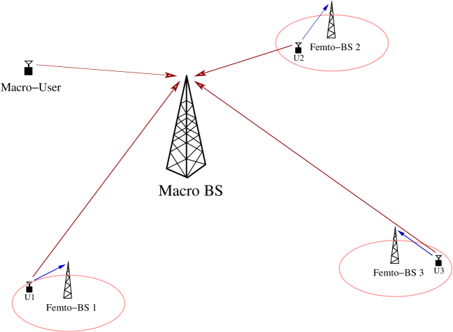
Figure 3: Modeling of uplink transmissions in a heterogeneous network (HetNet) with macro-BS and femto-BSs as a many-to-one X channel.

Small cells are seen as an effective means to achieve 3G data off-loading, and many mobile service providers consider small cells as a vital element for managing LTE Advanced spectrum more efficiently compared to using just macrocells. It is in this context that the knowledge of the optimality of different transmission strategies that the users can employ becomes valuable. Femto, pico and micro cells are also used to motivate a slightly similar channel model studied in [15], where a MAC generates interference for a single user uplink transmission. We note that the many-to-one IC was also motivated by considering a similar scenario where multiple short-range peer-to-peer communications create interference for a long-range receiver [11, 12].

We use a $3\times 3$ many-to-one XC to evaluate the different strategies. The sum-rate at all the receivers is used as the criterion for optimality. In general, we use genie-aided bounding techniques to derive the sum-rate capacity results in this paper. Specifically, for certain strategies we make use of the concepts of useful genie and smart genie introduced in [7]. A genie is said to be useful if it results in a genie-aided channel whose sum-rate capacity is achieved by Gaussian inputs, while a smart genie is one which does not increase the sum-rate when Gaussian inputs are used [7]. In [7], the genie-aided bounding technique is used to identify the regime under which all the interference can be treated as noise. In our work, we use this technique for scenarios where interference from a subset of transmitters is treated as noise. We show that strategies $\mathcal{M}1$ and $\mathcal{M}2$ achieve sum-rate capacity under certain channel conditions. For strategy $\mathcal{M}3$, we characterize the gap between the achievable sum-rate of the strategy and a sum-rate outer bound. Later, we extend these results to the $K\times K$ case.

Next, we identify a region in which the many-to-one XC can be operated as a many-to-one IC without loss of sum-rate and show that using Gaussian codebooks and treating interference as noise achieves a rate point that is within $K/2-1$ bits from the sum-rate capacity. In the last part of the paper, we observe some implications of the above results for the many-to-one IC. Firstly, we note that strategies similar to the ones defined above can be considered for the many-to-one IC as well. These involve a combination of partial interference cancellation and treating the rest of the interference as noise. We derive the sum-rate optimality of these strategies under certain channel conditions. Secondly, we identify a region for the many-to-one IC where the sum-rate capacity can be characterized to $K/2-1$ bits.

In this paper, we restrict ourselves to the many-to-one topology. In general, for the fully connected $K\times K$ XC, obtaining regions where conventional transmission strategies are sum-rate capacity optimal is difficult. However, some gap-to-capacity results have recently been obtained in [16, 17, 18, 19]. In [16], channel conditions under which treating interference as noise at the receivers (strategy $\mathcal{M}1$) achieves the entire channel capacity region of the $K$-user Gaussian interference channel to within a constant gap are obtained. This result is extended to the $K\times K$ XC in [17, 18] to show that under the same channel conditions, treating interference as noise is optimal in terms of sum-rate capacity up to a constant gap. In [19], a constant gap capacity approximation for the $2\times 2$ XC subject to an outage set has been obtained.

The rest of this paper is organized as follows. The system model is presented in Section II. In Section III, we consider the $3\times 3$ many-to-one XC and analyze the different strategies defined earlier. These results are extended to the $K\times K$ case in Section IV. Some implications of the above results for the Gaussian many-to-one IC are discussed in Section V. Numerical results and illustrations regarding the optimality of the strategies are presented in Section VI. Conclusions are presented in Section VII.

II System Model

As shown in Fig. 1, the many-to-one XC with $K$ transmitters and $K$ receivers is described by the following input-output equations

$$y_{1} = h_{11}\,\tilde{x}_{1}+\sum_{j=2}^{K}h_{1j}\,\tilde{x}_{j}+\,n_{1}$$ (1)

$$y_{i} = h_{ii}\,\tilde{x}_{i}+\,n_{i},\qquad\qquad\qquad i=2,3,\ldots,K,$$ (2)

where $\tilde{x}_{t}$ is the transmitted symbol by transmitter $t$, $h_{rt}$ denotes the channel coefficient from transmitter $t$ to receiver $r$, and $n_{r}$ is the additive Gaussian noise at receiver $r$. $h_{ii}$, $i=2,\ldots,K$, are the direct channels, while $h_{1i}$ are the cross channels. The additive noise $n_{r}$ is a zero mean Gaussian random variable with unit variance, i.e., $n_{r}\sim\mathcal{N}(0,1)$, $r=1,2,\ldots,K$.

Figure 4: Many-to-one X channel with $K$ transmitters in standard form.

II-A $K\times K$ Many-to-one X channel in standard form

The $K\times K$ many-to-one XC can be written in standard form (see Fig. 4), i.e.,

$$y_{1} = x_{1}+\sum_{j=2}^{K}h_{j}\,{x}_{j}+\,n_{1}$$ (3)

$$y_{i} = {x}_{i}+\,n_{i},\qquad i=2,3,\ldots,K,$$ (4)

where we have used $h_{j}=h_{ij}\,/\,h_{jj}$, $x_{i}=h_{ii}\,\tilde{x}_{i}$, and $P_{i}=|h_{ii}|^{2}\tilde{P}_{i}$ are the new power constraints [1].

As shown in Fig. 4, the $K\times K$ many-to-one XC has $2K-1$ independent messages, i.e., {$W_{11}$, $W_{12}$, $W_{22}$, $W_{13}$, $W_{33}$, …, $W_{1K}$, $W_{KK}$}, where $W_{ij}$ is the message transmitted from transmitter $j$ to receiver $i$.

We assume that the transmitter communicates the intended messages in $n$ channel uses. For a given block length $n$, we define a $\big{(}n,R_{11}\big{)}$ codebook at transmitter 1, and $\big{(}n,R_{ii},R_{1i}\big{)}$ codebook at transmitter $i$, $i=2,\ldots,K$, as follows:

1. Transmitter 1 communicates message $W_{11}\in\mathcal{W}_{11}=\{1,\ldots,2^{nR_{11}}\}$, while Transmitter $i$ communicates messages $W_{ii}\in\mathcal{W}_{ii}=\{1,\ldots,2^{nR_{ii}}\}$ and $W_{1i}\in\mathcal{W}_{1i}=\{1,\ldots,2^{nR_{1i}}\}$, $i=2,\ldots,K$.

2. An encoding function $f_{1}(\cdot)$ at transmitter $1$ maps the message $W_{11}$ to the transmitted codeword ${\bf x}_{1}^{n}=(x_{11},x_{12},\ldots,x_{1n})$, $f_{1}\,:\,(W_{ii},W_{1i})\rightarrow{\bf x}_{1}^{n}$ for each $W_{11}\in\mathcal{W}_{11}$. Similarly, for transmitter $i$, an encoding function $f_{i}(\cdot)$ maps the messages to the transmitted codewords, $f_{i}\,:\,(W_{ii},W_{1i})\rightarrow{\bf x}_{i}^{n}$ for each $(W_{ii},W_{1i})\in\mathcal{W}_{ii}\times\mathcal{W}_{1i}$, for $i=2,\ldots,K$.

3. The codewords in each codebook must satisfy the average power constraint $\frac{1}{n}\big{\|}{\bf x}_{i}^{n}\big{\|}_{2}^{2}\leq P_{i}$ at transmitter $i=1,\ldots,K$.

4. Receiver $i$ observes the channel outputs ${\bf y}_{i}^{n}=(y_{i1},y_{i2},\ldots,y_{in})$ and uses a decoding function $\phi_{k}(\cdot)$ at receiver $k$ which maps the received symbols to an estimate of the message: $\phi_{1}({\bf y}_{1})=(\hat{W}_{11},\hat{W}_{12},\ldots,\hat{W}_{1K})$ and $\phi_{k}({\bf y}_{k})=\hat{W}_{kk}$ for $k=2,\ldots,K$.

5. The average probability of error at receiver $k$, $P_{e,k}^{(n)}$ is given by

   $$P_{e,1}^{(n)} = \mathbb{E}\left[\text{Pr}\left(\big{(}\hat{W}_{11},\hat{W}_{12},\ldots,\hat{W}_{1K}\big{)}\neq({W}_{11},{W}_{12},\ldots,{W}_{1K}\big{)}\right)\right]$$

   $$P_{e,k}^{(n)} = \mathbb{E}\left[\text{Pr}\big{(}\hat{W}_{kk}\neq{W}_{kk}\big{)}\right],\qquad k=2,\ldots,K,$$

   where the expectation is taken with respect to the random choice of the transmitted messages.

We say that the rate vector $(R_{11},R_{12},\ldots,R_{1K},R_{22},\ldots R_{KK})$ is achievable for the $K\times K$ many-to-one XC if there exists a $\big{(}n,R_{11}\big{)}$ codebook at transmitter 1 satisfying the power constraint $P_{1}$, and $\big{(}n,R_{ii},R_{1i}\big{)}$ codebook at transmitter $i$ satisfying the power constraint $P_{i}$, $i=2,\ldots,K$, and decoding functions $(\phi_{1}(\cdot),\ldots,\phi_{K}(\cdot))$, such that the average decoding error probabilities $(P_{e,1}^{(n)},\ldots,P_{e,K}^{(n)})$ go to zero as block length $n$ goes to infinity. The capacity region is defined as the closure of the set of all achievable rate vectors $(R_{11},R_{12},\ldots,R_{1K},R_{22},\ldots R_{KK})$ and is denoted by $\mathcal{C}$. Then the sum-rate capacity $S$ of the $K\times K$ many-to-one XC is defined as

$$S = \max_{(R_{11},R_{12},\ldots,R_{1K},R_{22},\ldots R_{KK})\,\in\,\mathcal{C}}\Big{(}R_{11}+\sum_{i=2}^{K}(R_{ii}+R_{1i})\Big{)}.$$

By Fano’s inequality, we have

$$H(W_{ii}\,|\,{\bf y}_{i}^{n}) \leq n\epsilon_{n},\quad i=1,\ldots,K,$$

$$H(W_{1j}\,|\,{\bf y}_{1}^{n}) \leq n\epsilon_{n},\quad j=2,\ldots,K,$$ (5)

where $\epsilon_{n}\rightarrow 0$ as $n\rightarrow\infty$.

Next, in Lemma 1 below, we show that the $K\times K$ many-to-one XC is degraded under specific channel conditions. This lemma will later be used to prove the decodability of message sets at the receivers. In order for the result to be applicable to a more general case, we assume that the noise variance at each receiver is $\sigma_{i}^{2}$, $i=1,\ldots,K$.

Lemma 1

For the $K\times K$ many-to-one XC in standard form shown in Fig. 4 with noise variance $\sigma_{i}^{2}$ at receiver $i$, if $h_{i}^{2}\,\sigma_{i}^{2}\leq\sigma_{1}^{2}$, $i=2,\ldots,K$, then $y_{1}$ is a degraded version of $y_{i}$ with respect to message $W_{1i}$ and hence $H(W_{1i}\,|\,{\bf y}_{i}^{n})\leq n\epsilon_{n}$, where $\epsilon_{n}\rightarrow 0$ as $n\rightarrow\infty$. This implies that message $W_{1i}$ is decodable at receiver $i$. Furthermore, $H(W_{1i},W_{ii}\,|\,{\bf y}_{i}^{n})\leq 2n\epsilon_{n}$.

Proof:

At receiver 1, we have $y_{1}=x_{1}+\sum_{j=2}^{K}h_{j}\,{x}_{j}+\,n_{1}$, and at receiver $i$, we have $y_{i}=x_{i}+n_{i}$. Define $\tilde{y}_{1}=h_{i}x_{i}+n_{1}$ and $y_{1}^{\prime}=\tilde{y}_{1}/h_{i}=x_{i}+n_{1}^{\prime}$, where $n_{1}^{\prime}=n_{1}/h_{i}$. If $\sigma_{i}^{2}\leq\sigma_{1}^{2}/h_{i}^{2}$, we note that the noise variance of $n_{1}^{\prime}$ is higher than that of $n_{i}$. Hence $y_{1}^{\prime}$ is a stochastically degraded version of the signal $y_{i}$ received at receiver $i$. Thus, from the data processing inequality, we have $I(W_{1i}\,;\,{\bf y}_{i}^{n})\geq I(W_{1i}\,;\,{\bf y}_{1}^{\prime n})$. Since scaling the output of a channel does not affect its capacity, we have $I(W_{1i}\,;\,{\bf y}_{i}^{n})\geq I(W_{1i}\,;\,\tilde{\bf y}_{1}^{n})$. Therefore,

$$H(W_{1i}\,|\,{\bf y}_{i}^{n}) \leq H(W_{1i}\,|\,\tilde{\bf y}_{1}^{n})$$ (6)

$$\stackrel{{\scriptstyle(a)}}{{=}} H(W_{1i}\,|\,\tilde{\bf y}_{1}^{n},{\bf x}_{1}^{n},\ldots,{\bf x}_{i-1}^{n},{\bf x}_{i+1}^{n},\ldots,{\bf x}_{K}^{n}).$$

$$= H(W_{1i}\,|\,{\bf y}_{1}^{n},{\bf x}_{1}^{n},\ldots,{\bf x}_{i-1}^{n},{\bf x}_{i+1}^{n},\ldots,{\bf x}_{K}^{n}).$$

$$\stackrel{{\scriptstyle(b)}}{{\leq}} H(W_{1i}\,|\,{\bf y}_{1}^{n})$$

$$\stackrel{{\scriptstyle(c)}}{{\leq}} n\epsilon_{n},$$

where $(a)$ follows since $\big{(}{\bf x}_{1}^{n},\ldots,{\bf x}_{i-1}^{n},{\bf x}_{i+1}^{n},\ldots,{\bf x}_{K}^{n}\big{)}$ are independent of $W_{1i}$ and $\tilde{\bf y}_{1}^{n}$, $(b)$ follows from the fact that removing conditioning does not reduce the conditional entropy, and $(c)$ follows from (5). Thus, we conclude that $W_{1i}$ is decodable at receiver $i$ when $h_{i}^{2}\,\sigma_{i}^{2}\leq\sigma_{1}^{2}$. Note that in this case

$$H(W_{1i},W_{ii}\,|\,{\bf y}_{i}^{n}) = H(W_{1i}\,|\,{\bf y}_{i}^{n})+H(W_{ii}\,|\,{\bf y}_{i}^{n},W_{1i})$$ (7)

$${\leq} H(W_{1i}\,|\,{\bf y}_{i}^{n})+H(W_{ii}\,|\,{\bf y}_{i}^{n})$$

$$\leq 2n\epsilon_{n},$$

where (7) follows from (5) and (6). As $n\rightarrow\infty$, $\epsilon_{n}\rightarrow 0$. This shows that $(W_{ii},W_{1i})$ are decodable at receiver $i$. ∎

II-B $3\times 3$ Many-to-one X channel

In order to analyze the strategies, we first consider the $3\times 3$ many-to-one XC since the $2\times 2$ case results in the Z channel. The Z channel is obtained from the many-to-one XC by retaining only the first two transmitters and removing the rest. In this way, the many-to-one XC can be considered as one possible generalization of the Z channel. The Z channel has been studied in [20, 21].

The $3\times 3$ many-to-one XC channel can be written in standard form (See Fig. 5), i.e.,

$$y_{1} = x_{1}+ax_{2}+bx_{3}+\,n_{1}$$ (8)

$$y_{2} = \,x_{2}+\,n_{2}$$ (9)

$$y_{3} = \,x_{3}+\,n_{3},$$ (10)

where we have used $h_{2}=a$ and $h_{3}=b$.

As shown in Fig. 5, the $3\times 3$ many-to-one XC has five independent messages, $W_{11}$, $W_{12}$, $W_{13}$, $W_{22}$ and $W_{33}$, where $W_{ij}$ is the message transmitted from transmitter $j$ to receiver $i$.

Figure 5: Many-to-one X channel with $3$ transmitters in standard form.

Our motivation for considering the $3\times 3$ many-to-one XC first, instead of directly analyzing $K\times K$ case stems from three perspectives: (i) ease of presentation, (ii) understanding the proof techniques without cumbersome notational details, (iii) better visualization of the regions where the strategies are optimal (as seen in the numerical results presented in Section VI).

III Analysis of Different Strategies for the $3\times 3$ Many-to-One XC

We introduce some terminology useful in deriving the results in this section. Let ${\bf y}_{i}^{n}$ denote the vector of received symbols of length $n$ at receiver $i$. Let ${\bf x}_{i}^{n}$ denote the $n$ length vector of transmitted symbols at transmitter $i$. By Fano’s inequality, we have

$$H(W_{ii}\,|\,{\bf y}_{i}^{n}) \leq n\epsilon_{n},\quad i=1,2,3$$

$$H(W_{1j}\,|\,{\bf y}_{1}^{n}) \leq n\epsilon_{n},\quad j=2,3,$$ (11)

where $\epsilon_{n}\rightarrow 0$ as $n\rightarrow\infty$.

Before we proceed to analyze the various strategies, we provide a restatement of Lemma 5 in [7], in a form that is easier to apply to the many-to-one X channel. We make use of the following lemma to bound the sum-rate of the many-to-one XC in some cases.

Lemma 2

Let ${\bf w}_{i}^{n}$ be a sequence with average power constraint $\text{trace}(\mathbb{E}({\bf w}_{i}^{n}{\bf w}_{i}^{nT}))\leq nP_{i}$. Let ${\bf n}_{i}^{n}$, $i\neq 1$, be a random vector with components that are distributed as independent $\mathcal{N}(0,1)$ random variables. Let ${\bf n}_{1}^{n}$ denote a random vector with components that are distributed as independent $\mathcal{N}(0,\sigma^{2})$ random variables. Assume that ${\bf w}_{i}^{n}$ are independent of each other and also independent of ${\bf n}_{i}^{n}$. Let $w_{iG}\sim\mathcal{N}(0,P_{i})$. For some constants $c_{i}$, we have

$$\sum_{i=1}^{K}h({\bf w}_{i}^{n}+{\bf n}_{i}^{n})-h\Big{(}\sum_{i=1}^{K}c_{i}\,{\bf w}_{i}^{n}+{\bf n}_{1}^{n}\Big{)} \leq n\sum_{i=1}^{K}h({w}_{iG}+{n}_{i})-nh\Big{(}\sum_{i=1}^{K}c_{i}\,{w}_{iG}+{n}_{1}\Big{)},\quad$$ (12)

when $\sum_{i=1}^{K}c_{i}^{2}\leq{\sigma^{2}}$ and equality is achieved if ${\bf w}_{i}^{n}={\bf w}_{iG}^{n}$, where ${\bf w}_{iG}^{n}$ denotes a complex random vector with components that are i.i.d $\mathcal{N}(0,P_{i})$.

Proof:

Let ${\bf t}^{n}_{i}=c_{i}({\bf w}_{i}^{n}+{\bf n}_{i}^{n})$. The left-hand side of (12) can now be written as

$$\sum_{i=1}^{K}h({\bf t}^{n}_{i})-h\Big{(}\sum_{i=1}^{K}{\bf t}^{n}_{i}+\tilde{\bf n}_{1}^{n}\Big{)}+n\sum_{i=1}^{K}\log c_{i},$$

where $\tilde{\bf n}_{1}^{n}$ is a random vector with components that are i.i.d $\mathcal{N}\big{(}0,{\sigma^{2}}-\sum_{i=1}^{K}c_{i}^{2}\big{)}$. The final result follows by applying Lemma 5 in [7], i.e.,

$$\sum_{i=1}^{K}h({\bf t}^{n}_{i})-h\Big{(}\sum_{i=1}^{K}{\bf t}^{n}_{i}+\tilde{\bf n}_{1}^{n}\Big{)} \leq \;n\sum_{i=1}^{K}h({t}_{iG})-nh\Big{(}\sum_{i=1}^{K}{t}_{iG}+\tilde{n}_{1}\Big{)},$$

where $t_{iG}=c_{i}({w}_{iG}+{n}_{i})$ and equality is achieved if ${\bf w}_{i}^{n}={\bf w}_{iG}^{n}$. Since the variance of $\tilde{n}_{1}$ cannot be negative, we have the condition $\sum_{i=1}^{K}c_{i}^{2}\leq{\sigma^{2}}$. ∎

III-A Optimality of Strategy $\mathcal{M}1$

Transmitter/	Transmitted	Decoded
Receiver index	messages	messages
1	$W_{11}$	$\widehat{W}_{11}$
2	$W_{22}$	$\widehat{W}_{22}$
3	$W_{33}$	$\widehat{W}_{33}$

TABLE II: Transmitted and Decoded messages for strategy $\mathcal{M}1$

The transmitted and decoded messages in strategy $\mathcal{M}1$ are illustrated in Table II. In strategy $\mathcal{M}1$, we are interested in a region where sum-rate capacity is achieved by using Gaussian codebooks and treating interference as noise. This is usually referred to as the low-interference or the noisy-interference regime in the interference channel literature. In strategy $\mathcal{M}1$, cross messages in the channel are not utilized, i.e., $W_{12}=W_{13}=\phi$. We characterize the noisy-interference sum-rate capacity in the following theorem.

Theorem 1

For the $3\times 3$ Gaussian many-to-one XC, strategy $\mathcal{M}1$ achieves sum-rate capacity if

$$a^{2}+b^{2} \leq 1,$$ (13)

and the sum-rate capacity is given by

$$S = 0.5\log\bigg{(}1+\frac{P_{1}}{1+a^{2}P_{2}+b^{2}P_{3}}\bigg{)}+0.5\log(1+P_{2})+0.5\log(1+P_{3}).$$ (14)

Proof:

If $b^{2}\leq 1$, from Lemma 1, we have $H(W_{13}\,|\,{\bf y}_{3}^{n})\leq n\epsilon_{n}$ and $H(W_{13},W_{33}\,|\,{\bf y}_{3}^{n})\leq 2n\epsilon_{n}$. Similarly, if $a^{2}\leq 1$, $W_{12}$ is decodable at receiver 2, i.e., $H(W_{12}\,|\,{\bf y}_{2}^{n})\leq n\epsilon_{n}$ and $H(W_{12},W_{22}\,|\,{\bf y}_{2}^{n})\leq 2n\epsilon_{n}$.

Now, assume $a^{2}\leq 1$ and $b^{2}\leq 1$. The sum-rate can be bounded as follows:

$$nS \leq H(W_{11})+H(W_{12},W_{22})+H(W_{13},W_{33})$$

$$= {I(W_{11}\,;\,{\bf y}_{1}^{n})+\sum_{i=2}^{3}I(W_{1i},W_{ii}\,;\,{\bf y}_{i}^{n})+H(W_{11}\,|\,{\bf y}_{1}^{n})+\sum_{i=2}^{3}H(W_{1i},W_{ii}\,|\,{\bf y}_{i}^{n})}$$

$$\leq {I({\bf x}_{1}^{n}\,;\,{\bf y}_{1}^{n})+\sum_{i=2}^{3}I({\bf x}_{i}^{n}\,;\,{\bf y}_{i}^{n})+H(W_{11}\,|\,{\bf y}_{1}^{n})+\sum_{i=2}^{3}H(W_{1i},W_{ii}\,|\,{\bf y}_{i}^{n})}$$

$$\stackrel{{\scriptstyle(a)}}{{\leq}} h({\bf y}_{1}^{n})-h(a\;\!{\bf x}_{2}^{n}+b\;\!{\bf x}_{3}^{n}+{\bf n}_{1}^{n})+h({\bf x}_{2}^{n}+{\bf n}_{2}^{n})-h({\bf n}_{2}^{n})+h({\bf x}_{3}^{n}+{\bf n}_{3}^{n})-h({\bf n}_{3}^{n})+5\epsilon_{n}$$

$$\stackrel{{\scriptstyle(b)}}{{\leq}} nh({y}_{1G})+nh({x}_{2G}+{n}_{2})+nh({x}_{3G}+{n}_{3})-nh(a\;\!{x}_{2G}+b\;\!{x}_{3G}+{n}_{1})-nh(n_{2})$$

$$-nh(n_{3})+5\epsilon_{n}$$

$$= nI({x}_{1G};{y}_{1G})+nI({x}_{2G};{y}_{2G})+nI({x}_{3G};{y}_{3G})+5\epsilon_{n},$$

where $x_{iG}\sim\mathcal{N}(0,P_{i})$, $y_{iG}$ denotes $y_{i}$ with $x_{j}=x_{jG}$, $\forall\,i,j$, $(a)$ follows from (11), and from the application of Lemma 1, and in $(b)$, we have used Lemma 2 to bound the term $h({\bf x}_{2}^{n}+{\bf n}_{2}^{n})+h({\bf x}_{3}^{n}+{\bf n}_{3}^{n})-h(a{\bf x}_{2}^{n}+b{\bf x}_{3}^{n}+{\bf n}_{1}^{n})$, under the condition $a^{2}+b^{2}\leq 1$. As $n\rightarrow\infty$, $\epsilon_{n}\rightarrow 0$, and we have

$$S {\leq} 0.5\log\bigg{(}1+\frac{P_{1}}{1+a^{2}P_{2}+b^{2}P_{3}}\bigg{)}+\sum_{i=2}^{3}0.5\log(1+P_{i}).\quad$$ (15)

This sum-rate bound can be achieved using strategy $\mathcal{M}1$. We observe that the sum-rate bound in (15) is also achievable in the $3\times 3$ many-to-one IC by using Gaussian inputs and treating interference at receiver 1 as noise. Note that in the $3\times 3$ many-to-one IC, the cross messages $W_{12}$ and $W_{13}$ are absent. Since the many-to-one IC is a special case of the many-to-one XC, this shows that the presence of cross messages does not improve the sum-rate when $a^{2}+b^{2}\leq 1$. This means that we can set $W_{12}=W_{13}=\phi$ in the $3\times 3$ many-to-one XC without loss of sum-rate. ∎

Remark 1

Theorem 1 was proved for the many-to-one interference channel in [7, Theorem 4] using genie aided bounding techniques. The low-interference regime for the discrete memoryless many-to-one interference channels is proved in [10]. We also note that the result in [7] is a special case of a more general result in [22, Theorem 3], where the sum-rate capacity of a $K$-user Gaussian interference channel is characterized in the noisy-interference regime.

III-B Optimality of Strategy $\small\mathcal{M}2$

Transmitter/	Case I		Case II
Receiver	Transmitted	Decoded	Transmitted	Decoded
index	messages	messages	messages	messages
1	$W_{11}$	$\widehat{W}_{11}$, $\widehat{W}_{12}$	$W_{11}$	$\widehat{W}_{11}$, $\widehat{W}_{13}$
2	$W_{12}$	-	$W_{22}$	$\widehat{W}_{22}$
3	$W_{33}$	$\widehat{W}_{33}$	$W_{13}$	-

TABLE III: Transmitted and Decoded messages for strategy $\mathcal{M}2$

The transmitted and decoded messages in strategy $\mathcal{M}2$ are illustrated in Table III. Here, we ask the following question: are there channel conditions such that the sum-rate capacity is achieved by a two-user MAC at receiver 1 formed by transmitter 1 and either transmitter 2 (case I) or transmitter 3 (case II), while the interference from the other transmitter is treated as noise? Observe that the other transmitter forms a point-to-point channel and is a source of interference for the two-user MAC. We characterize the sum-rate capacity in the following theorem.

Theorem 2

For the $3\times 3$ Gaussian many-to-one XC, the sum-rate capacity is achieved by strategy $\mathcal{M}2$, where a two-user MAC is formed by transmitter 1 and either transmitter 2 or transmitter 3 at receiver 1, for the following channel conditions, respectively

1. $a^{2}\;\;\geq\;\;\displaystyle\frac{(1+b^{2}P_{3})^{2}}{{1-b^{2}}},\quad\;\,b^{2}\;<\;1$

2. $b^{2}\;\;\geq\;\;\displaystyle\frac{(1+a^{2}P_{2})^{2}}{1-a^{2}},\quad\;\,a^{2}\;<\;1$.

Proof:

We prove statement (i) below. This represents case I in Table III, where transmitters 1 and 2 form a MAC at receiver 1 while interference from transmitter 3 is treated as noise. The proof for the second statement which corresponds to case II in Table III follows along similar lines.

We use genie-aided bounding techniques to derive the optimality of strategy $\mathcal{M}2$. Specifically, we use the concept of useful genie and smart genie introduced in [7] to obtain the sum-rate capacity for strategy $\mathcal{M}2$. Let a genie provide the following side information to receiver 1:

$$s_{1} = x_{1}+a\,x_{2}+\eta\,z_{1},$$ (16)

where $z_{1}\sim\mathcal{N}(0,1)$ and $\eta$ is a positive real number. We allow $z_{1}$ to be correlated to $n_{1}$ with correlation coefficient $\rho$.

A genie is said to be useful if it results in a genie-aided channel whose sum-rate capacity is achieved by Gaussian inputs, i.e., the sum-rate capacity of the genie-aided channel equals $I({x}_{1G},\,{x}_{2G}\,;\,{y}_{1G},{s}_{1G})+I({x}_{3G}\,;\,{y}_{3G})$, where $x_{iG}\sim\mathcal{N}(0,P_{i})$, $y_{iG}$, $s_{1G}$ are $y_{i}$ and $s_{1}$ with $x_{j}=x_{jG}$, $\forall\,i,j$.

Lemma 3

(Useful Genie) The sum-rate capacity of the genie-aided channel with side information (16) given to receiver 1 is achieved by using Gaussian inputs and by treating interference from transmitter 3 as noise at receiver 1, if the following conditions hold:

$$\eta^{2}\;\leq\;a^{2}, b^{2}\;\leq\;1-\rho^{2},$$ (17)

and the sum-rate of the genie-aided channel is bounded as

$$S \leq I({x}_{1G},\,{x}_{2G}\,;\,{y}_{1G},{s}_{1G})+I({x}_{3G}\,;\,{y}_{3G}).$$ (18)

Proof:

The sum-rate of the genie-aided channel can be bounded as

$$nS \leq H(W_{11},W_{12},W_{22})+H(W_{13},W_{33})$$ (19)

$$= I(W_{11},W_{12},W_{22}\,;\,{\bf y}_{1}^{n},\,{\bf s}_{1}^{n})+H(W_{11}\,|\,{\bf y}_{1}^{n},\,{\bf s}_{1}^{n})+H(W_{12}\,|\,{\bf y}_{1}^{n},\,{\bf s}_{1}^{n},{\bf x}_{1}^{n})$$

$$+\,H(W_{22}\,|\,{\bf y}_{1}^{n},\,{\bf s}_{1}^{n},{\bf x}_{1}^{n},W_{12})+I(W_{13},W_{33};{\bf y}_{3}^{n})\!+\!H(W_{13}|{\bf y}_{3}^{n})\!+\!H(W_{33}|{\bf y}_{3}^{n},W_{13})$$

$$\stackrel{{\scriptstyle(a)}}{{\leq}} I({\bf x}_{1}^{n},\,{\bf x}_{2}^{n}\,;\,{\bf y}_{1}^{n},\,{\bf s}_{1}^{n})+{H(W_{11}\,|\,{\bf y}_{1}^{n})}+\,H(W_{12}\,|\,{\bf y}_{1}^{n})$$

$$+\,H(W_{22}\,|\,{\bf s}_{1}^{n},\,{\bf x}_{1}^{n})+I({\bf x}_{3}^{n}\,;\,{\bf y}_{3}^{n})+\,H(W_{13}\,|\,{\bf y}_{3}^{n})+H(W_{33}\,|\,{\bf y}_{3}^{n}),$$

where $(a)$ follows from the fact that removing conditioning cannot reduce the conditional entropy.

We bound the term $H(W_{22}\,|\,{\bf s}_{1}^{n},\,{\bf x}_{1}^{n})$. If $\eta^{2}\leq a^{2}$, then we have $I(W_{22}\,;\,{\bf s}_{1}^{n}\,|\,{\bf x}_{1}^{n})\geq I(W_{22}\,;\,{\bf y}_{2}^{n})$. Thus,

$$H(W_{22}\,|\,{\bf s}_{1}^{n},\,{\bf x}_{1}^{n}) \leq H(W_{22}\,|\,{\bf y}_{2}^{n})$$ (20)

$$\leq n\epsilon_{n}.$$

From Lemma 1, we have $H(W_{13}\,|\,{\bf y}_{3}^{n})\leq n\epsilon_{n}$ when $b^{2}\leq 1$. Using (11) and (20) in (19), we have

$$nS \leq I({\bf x}_{1}^{n},{\bf x}_{2}^{n}\,;\,{\bf y}_{1}^{n},\,{\bf s}_{1}^{n})+I({\bf x}_{3}^{n}\,;\,{\bf y}_{3}^{n})+5n\epsilon_{n}$$

$$= I({\bf x}_{1}^{n},{\bf x}_{2}^{n};{\bf s}_{1}^{n})\!+I({\bf x}_{1}^{n},{\bf x}_{2}^{n};{\bf y}_{1}^{n}\,|\,{\bf s}_{1}^{n})\!+I({\bf x}_{3}^{n};{\bf y}_{3}^{n})+5n\epsilon_{n}$$

$$= h({\bf s}_{1}^{n})-h({\bf s}_{1}^{n}\,|\,{\bf x}_{1}^{n},{\bf x}_{2}^{n})+h({\bf y}_{1}^{n}\,|\,{\bf s}_{1}^{n})$$

$$-\,h({\bf y}_{1}^{n}\,|\,{\bf s}_{1}^{n},{\bf x}_{1}^{n},{\bf x}_{2}^{n})+h({\bf y}_{3}^{n})-h({\bf y}_{3}^{n}\,|\,{\bf x}_{3}^{n})+5n\epsilon_{n}$$

$$= h({\bf s}_{1}^{n})-h(\eta\,{\bf z}_{1}^{n})+h({\bf y}_{1}^{n}\,|\,{\bf s}_{1}^{n})-h(b\,{\bf x}_{3}^{n}+{\bf n}_{1}^{n}\,|\,{\bf z}_{1}^{n})+\,h({\bf y}_{3}^{n})-h({\bf n}_{3}^{n})+5n\epsilon_{n}$$

$$\stackrel{{\scriptstyle(b)}}{{\leq}} nh({s}_{1G})-nh(\eta\,{z}_{1})+{nh({y}_{1G}\,|\,{s}_{1G})}$$

$$-\,h(b\,{\bf x}_{3}^{n}+\tilde{\bf n}_{1}^{n})+h({\bf x}_{3}^{n}+{\bf n}_{3}^{n})-nh({n}_{3})+5n\epsilon_{n}$$

$$\stackrel{{\scriptstyle(c)}}{{\leq}} nh({s}_{1G})-nh(\eta\,{z}_{1})+{nh({y}_{1G}\,|\,{s}_{1G})}$$

$$+\,nh({x}_{3G}+{n}_{3})-nh(b\,{x}_{3G}+\tilde{n}_{1})-nh({n}_{3})+5n\epsilon_{n}$$

$$= n\,I({x}_{1G},{x}_{2G}\,;\,{y}_{1G},\,{s}_{1G})+n\,I({x}_{3G}\,;\,{y}_{3G})+5n\epsilon_{n},$$

where $\tilde{n_{1}}\sim\mathcal{N}(0,1-\rho^{2})$, $(b)$ follows since Gaussian inputs maximize differential entropy for a given covariance constraint and from the application of Lemmas 1 and 6 in [7], $(c)$ follows from applying Lemma 1 in [6] (which is a special case of the extremal inequality considered in [23]) to the term $h({\bf x}_{3}^{n}+{\bf n}_{3}^{n})-\,h(b\,{\bf x}_{3}^{n}+\tilde{\bf n}_{1}^{n})$, and using the condition $b^{2}\;\leq\;1-\rho^{2}$. ∎

Next, we show that the genie is smart. A smart genie is one which does not improve the sum-rate when Gaussian inputs are used, i.e., $I({x}_{1G},\,{x}_{2G}\,;\,{y}_{1G},{s}_{1G})=I({x}_{1G},\,{x}_{2G}\,;\,{y}_{1G})$.

Lemma 4

(Smart Genie) If Gaussian inputs are used, and interference is treated as noise, then, under the condition

$$\eta\rho=1\;+\;b^{2}P_{3},$$ (21)

the genie does not increase the sum rate, i.e.,

$$I({x}_{1G},\,{x}_{2G}\,;\,{y}_{1G},\,{s}_{1G})=I({x}_{1G},\,{x}_{2G}\,;\,{y}_{1G}).$$ (22)

Proof:

Note that

$$I({x}_{1G},\,{x}_{2G}\,;\,{y}_{1G},{s}_{1G}) = I({x}_{1G},\,{x}_{2G}\,;\,{y}_{1G})+I({x}_{1G},\,{x}_{2G}\,;\,{s}_{1G}\,|\,{y}_{1G}).$$

The second term on the right hand side can be expanded as

$$I({x}_{1G}\,;\,{s}_{1G}\,|\,{y}_{1G})+I({x}_{2G}\,;\,{s}_{1G}\,|\,{y}_{1G},\,{x}_{1G}).$$

Consider

$$I({x}_{1G};{s}_{1G}\,|\,{y}_{1G}) = I({x}_{1G}\,;\,x_{1G}+a\,x_{2G}+\eta z_{1}\,|\,x_{1G}+a\,x_{2G}+b\,x_{3G}+n_{1}).$$

From Lemma 8 in [7], if $x$, $n$, $z$ are Gaussian with $x$ being independent of the two zero-mean random variables $n$, $z$, then $I(x\,;\,x+z\,|\,x+n)=0$, iff $\mathbb{E}(z\,n)=\mathbb{E}(n^{2})$. Thus, $I({x}_{1G};{s}_{1G}\,|\,{y}_{1G})$ becomes zero if $a^{2}P_{2}+\eta\,\rho=1+a^{2}P_{2}+b^{2}P_{3}$ which reduces to (21). Now, consider

$$I({x}_{2G}\,;\,{s}_{1G}\,|\,{y}_{1G},\,{x}_{1G}) = \;I({x}_{2G}\,;\,a\,x_{2G}+\eta\,z_{1}\,|\,a\,x_{2G}+b\,x_{3G}+n_{1})$$

$$\stackrel{{\scriptstyle(d)}}{{=}} 0.$$

where $(d)$ follows from [7, Lemma 8] and (21). ∎

Combining conditions (17) and (21), we have

$$a^{2}\;\;\geq\;\;\frac{(1+b^{2}P_{3})^{2}}{\rho^{2}} b^{2}\;\leq\;{1-\rho^{2}}.$$ ; (23)

For a fixed value of $b$, we have the constraint $\rho^{2}\leq{1-b^{2}}$. Note that choosing $\rho^{2}={1-b^{2}}$ results in the best bound for $a^{2}$. From (21), we infer that $\rho>0$, and using (17), this implies that $b^{2}<1$. Thus, (23) can be rewritten as statement (i) in Theorem 2. ∎

III-C Gap from optimality of Strategy $\small\mathcal{M}3$

Transmitter/	Transmitted	Decoded
Receiver index	messages	messages
1	$W_{11}$	$\widehat{W}_{11}$, $\widehat{W}_{12}$, $\widehat{W}_{13}$
2	$W_{12}$	-
3	$W_{13}$	-

TABLE IV: Transmitted and Decoded messages for strategy $\mathcal{M}3$

The transmitted and decoded messages in strategy $\mathcal{M}3$ are illustrated in Table IV. In strategy $\mathcal{M}3$, all transmitters form a MAC at receiver 1. We derive a sum-rate outer bound to the many-to-one XC and characterize the gap between the outer bound and the achievable sum-rate of strategy $\mathcal{M}3$.

Theorem 3

For the $3\times 3$ Gaussian many-to-one XC, when strategy $\mathcal{M}3$ is employed, if

$$a^{2}\,\,\geq\,\,\displaystyle\frac{(1+b^{2}P_{3})^{2}}{\rho^{2}} \;\,b^{2}\,\,\geq\,\,1,$$ and (24)

then the gap between the sum-rate outer bound and the sum-rate of strategy $\small\mathcal{M}3$ is given by

$$0.5\log\left(\frac{1-({1+b^{2}P_{3}})^{-1}\rho^{2}}{1-\rho^{2}}\right),$$ (25)

where $\rho$ denotes a constant with $\rho\in[-1,1]$.

Proof:

We use genie-aided techniques to derive the sum-rate outer bound. Let a genie provide the side information given in (16) to receiver 1. We prove below that the genie is useful.

Lemma 5

(Useful Genie) The sum-rate capacity of the genie-aided channel with side information (16) given to receiver 1 is achieved by using Gaussian inputs when all transmitters transmit to receiver 1, if the following conditions hold:

$$\eta^{2}\;\;\leq\;\;a^{2}, b^{2}\;\;\geq\;\;1,$$ (26)

and the sum-rate of the genie-aided channel is bounded as

$$S \leq I({x}_{1G},\,{x}_{2G},\,{x}_{3G}\,;\,{y}_{1G},{s}_{1G}).$$ (27)

Proof:

The sum-rate $S$ of the genie-aided channel is bounded as

$$nS \leq H(W_{11},W_{12},W_{13},W_{22},W_{33})$$ (28)

$$= {I(W_{11},W_{12},W_{13},W_{22},W_{33}\,;\,{\bf y}_{1}^{n},{\bf s}_{1}^{n})+H(W_{11},W_{12},W_{13},W_{22},W_{33}\,|\,{\bf y}_{1}^{n},{\bf s}_{1}^{n})}$$

$$= {I(W_{11},W_{12},W_{13},W_{22},W_{33}\,;\,{\bf y}_{1}^{n},{\bf s}_{1}^{n})}+H(W_{11}\,|\,{\bf y}_{1}^{n},{\bf s}_{1}^{n})+H(W_{12}\,|\,{\bf y}_{1}^{n},{\bf s}_{1}^{n},{\bf x}_{1}^{n})$$

$$+\,H(W_{22}|{\bf y}_{1}^{n},{\bf s}_{1}^{n},{\bf x}_{1}^{n},W_{12})+H(W_{13}|{\bf y}_{1}^{n},{\bf s}_{1}^{n},{\bf x}_{1}^{n},{\bf x}^{n}_{2})+H(W_{33}|{\bf y}_{1}^{n},{\bf s}_{1}^{n},{\bf x}_{1}^{n},{\bf x}^{n}_{2},W_{13})$$

$$\leq I({\bf x}_{1}^{n},{\bf x}_{2}^{n},{\bf x}_{3}^{n};{\bf y}_{1}^{n},{\bf s}_{1}^{n})+H(W_{11}|{\bf y}_{1}^{n})+H(W_{12}|{\bf y}_{1}^{n})+H(W_{22}|{\bf s}_{1}^{n},{\bf x}_{1}^{n})\!+\!H(W_{13}|{\bf y}_{1}^{n})$$

$$+H(W_{33}|{\bf y}_{1}^{n},{\bf x}_{1}^{n},{\bf x}^{n}_{2}).$$

We bound the term $H(W_{33}\,|\,{\bf y}_{1}^{n},{\bf x}_{1}^{n},{\bf x}_{2}^{n})$. If $b^{2}\geq 1$, then $I(W_{33};{\bf y}_{1}^{n}\,|\,{\bf x}_{1}^{n},{\bf x}_{2}^{n})\geq I(W_{33}\,;\,{\bf y}_{3}^{n})$. Therefore,

$$H(W_{33}\,|\,{\bf y}_{1}^{n},\,{\bf x}_{1}^{n},{\bf x}_{2}^{n}) \leq H(W_{33}\,|\,{\bf y}_{3}^{n})$$ (29)

$$\leq n\epsilon_{n}.$$

Note that the term $H(W_{22}\,|\,{\bf s}_{1}^{n},{\bf x}_{1}^{n})$ is again bounded as in (20) if $\eta^{2}\;\leq\;a^{2}$. Using (11), (20), and (29) in (28), we have

$$nS \leq I({\bf x}_{1}^{n},{\bf x}_{2}^{n},{\bf x}_{3}^{n};{\bf y}_{1}^{n},{\bf s}_{1}^{n})+5n\epsilon_{n}$$

$$= I({\bf x}_{1}^{n},{\bf x}_{2}^{n},{\bf x}_{3}^{n};{\bf y}_{1}^{n})+I({\bf x}_{1}^{n},{\bf x}_{2}^{n},{\bf x}_{3}^{n};{\bf s}_{1}^{n}\,|\,{\bf y}_{1}^{n})+5n\epsilon_{n}$$

$$\stackrel{{\scriptstyle(a)}}{{\leq}} nI({x}_{1G},{x}_{2G},{x}_{3G};{y}_{1G})+h({\bf s}_{1}^{n}\,|\,{\bf y}_{1}^{n})-h({\bf s}_{1}^{n}\,|\,{\bf y}_{1}^{n},{\bf x}_{1}^{n},{\bf x}_{2}^{n},{\bf x}_{3}^{n})+5\epsilon_{n}$$

$$\stackrel{{\scriptstyle(b)}}{{\leq}} nI({x}_{1G},{x}_{2G},{x}_{3G};{y}_{1G})+nh({s}_{1G}\,|\,{y}_{1G})-nh(\eta z_{1}\,|\,n_{1})+5\epsilon_{n}$$

$$= nI({x}_{1G},\,{x}_{2G},\,{x}_{3G}\,;\,{y}_{1G},{s}_{1G})+5\epsilon_{n},$$

where $(a)$ follows from the optimality of Gaussian inputs for Gaussian MAC, $(b)$ follows from Lemma 1 in [7]. Here, ${y}_{1G}$ denotes $y_{1}$ with $x_{i}$ being Gaussian distributed, i.e., ${y}_{1G}={x}_{1G}+a{x}_{2G}+b{x}_{3G}+{n}_{1}$. As $n\rightarrow\infty$, $\epsilon_{n}\rightarrow 0$ and we get the desired bound. ∎

Unlike in the case of strategy $\small\mathcal{M}2$, here the genie does in fact increase the sum-rate and hence is not smart. However, we can choose the parameters $\rho$ and $\eta$ to get a good sum-rate outer bound as follows. Consider

$$I({x}_{1G},\,{x}_{2G},\,{x}_{3G}\,;\,{y}_{1G},{s}_{1G}) = \;I({x}_{1G},{x}_{2G},{x}_{3G};{y}_{1G})+I({x}_{1G},{x}_{2G},{x}_{3G};{s}_{1G}\,|\,{y}_{1G}).$$

The second term on the right hand side can be expanded as

$$I({x}_{1G},\,{x}_{2G};{s}_{1G}\,|\,{y}_{1G})+I({x}_{3G}\,;\,{s}_{1G}\,|\,{y}_{1G},{x}_{1G},\,{x}_{2G}).$$ (30)

Strategy	Channel conditions	Gap from Outer-bound
$\normalsize\mathcal{M}1$	$a^{2}+b^{2}\leq 1$	0
$\normalsize\mathcal{M}2$	(i) $a^{2}\geq\displaystyle\frac{(1+b^{2}P_{3})^{2}}{1-b^{2}},\;\,{b^{2}<1}$	0
	(ii) $b^{2}\geq\displaystyle\frac{(1+a^{2}P_{2})^{2}}{1-a^{2}},\;\,{a^{2}<1}$	0
$\normalsize\mathcal{M}3$	(i) $a^{2}\,\geq\displaystyle\frac{(1+b^{2}P_{3})^{2}}{\rho^{2}},\;\,b^{2}\geq 1$	$0.5\log\Bigg{[}\displaystyle\frac{1-\displaystyle\frac{\rho^{2}}{1+b^{2}\,P_{3}}}{1-\rho^{2}}\Bigg{]}$
	(ii) $b^{2}\,\geq\displaystyle\frac{(1+a^{2}P_{2})^{2}}{\rho^{2}},\;\,a^{2}\geq 1$	$0.5\log\Bigg{[}\displaystyle\frac{1-\displaystyle\frac{\rho^{2}}{1+a^{2}\,P_{2}}}{1-\rho^{2}}\Bigg{]}$

TABLE V: Summary of results for many-to-one X channel

In the proof of Lemma 4, we showed that by choosing $\eta\,\rho=1+b^{2}P_{3}$, we can make $I({x}_{1G},\,{x}_{2G};{s}_{1G}\,|\,{y}_{1G})=0$. Now, consider

$$I({x}_{3G};{s}_{1G}\,|\,{y}_{1G},\,{x}_{1G},{x}_{2G}) = I({x}_{3G};\eta\,z_{1}\,|\,b\,x_{3G}+n_{1})$$ (31)

$$= h(\eta\,z_{1}\,|\,b\,x_{3G}+n_{1})-h(\eta\,z_{1}\,|\,n_{1})$$

$$\stackrel{{\scriptstyle(c)}}{{=}} h(\eta\,z_{1}\,|\,b\,x_{3G}+n_{1})-h(\eta\,\tilde{z}_{1})$$

$$= 0.5\log\left(\frac{\eta^{2}(1+b^{2}\,P_{3})-\eta^{2}\rho^{2}}{(1+b^{2}P_{3})\eta^{2}(1-\rho^{2})}\right)$$

$$= 0.5\log\left(\frac{1-({1+b^{2}P_{3}})^{-1}\rho^{2}}{1-\rho^{2}}\right)\!,$$

where $\tilde{z}_{1}\sim\mathcal{N}(0,1-\rho^{2})$ and $(c)$ follows from [7, Lemma 6]. Note that (31) represents the gap between the sum-rate outer bound and the sum-rate of strategy $\small\mathcal{M}3$. Combining condition (26) with $\eta\,\rho=1+b^{2}P_{3}$, we get (24). ∎

Due to the underlying symmetry in the MAC at receiver 1, a result corresponding to Theorem 3 with the channel coefficients $a$, $b$ and power levels $P_{2}$, $P_{3}$ interchanged is also true and further can be proved along similar lines. The results of this section are succinctly summarized in Table V.

III-D Recovering known results for the Z channel

We specialize the results in this section to the Z channel. The Z channel is obtained from the many-to-one X channel by retaining only the first two transmitters and removing the rest [20, 21]. In the $3\times 3$ many-to-one XC shown in Fig. 5, this is equivalent to setting $b=0$, and considering the outputs at the first two receivers alone. In this case, Theorem 1 reduces to the channel condition $a^{2}\leq 1$, which is identical to that obtained in [20] for the low-interference regime. Theorem 2 reduces to the condition $a^{2}\geq 1$, which is same as that obtained in [21] for the MAC sum-rate at receiver 1 to be the sum-rate capacity of the Z channel.

IV Extension to the $K\times K$ Many-to-One X Channel

Since the results for the $K\times K$ many-to-one XC follow more or less along similar lines as the $3\times 3$ case, we state the results along with a brief outline of the proof for each strategy, with additional details provided in places where the proofs differ.

IV-A Conditions for the sum-rate optimality of strategies $\mathcal{M}1$, $\mathcal{M}2$ and $\mathcal{M}3$

The optimality of strategy $\small\mathcal{M}1$ follows using similar arguments as in Theorem 1, under the condition $\sum_{i\,=\,2}^{K}h_{i}^{2}\leq 1$. This condition arises from the use of Lemma 2, as in inequality $(b)$ of Theorem 1. To avoid repeating the details, we omit the proof.

Next, we consider the optimality of strategy $\small\mathcal{M}2$. Here, we are interested in a region where the sum-rate capacity is achieved by a two-user MAC at receiver 1 formed by transmitter 1 and transmitter $k$, $k=2,\ldots,K$, while the interference from the other transmitters is treated as noise. In strategy $\small\mathcal{M}2$, the transmitted messages are $W_{ii}$ at transmitter $i$, $i\neq k$, and $W_{1k}$ at transmitter $k$. The decoded messages are $(\widehat{W}_{11},\widehat{W}_{1k})$ at receiver 1, and $\widehat{W}_{jj}$ at receiver $j$, $j\neq(1,k)$. We characterize the sum-rate capacity in the following theorem.

Theorem 4

For the $K\times K$ Gaussian many-to-one XC, the sum-rate capacity is achieved by the two-user MAC formed by transmitter 1 and transmitter $k$ to receiver 1, for the following channel conditions

$$h_{k}^{2} \geq \frac{\Big{(}1+\sum_{\begin{subarray}{c}j=2,\,j\neq k\end{subarray}}^{K}h_{j}^{2}P_{j}\Big{)}^{2}}{1-\sum_{\begin{subarray}{c}j=2,\,j\neq k\end{subarray}}^{K}h_{j}^{2}},$$

$${\sum_{\begin{subarray}{c}j=2,\,j\neq k\end{subarray}}^{K}h_{j}^{2}} < 1.$$ (32)

Proof:

Let a genie provide the following side information to receiver 1:

$$s_{k} = x_{1}+h_{k}\,x_{k}+\eta_{k}\,z_{k},$$ (33)

where $z_{k}\sim\mathcal{N}(0,1)$ and $\eta_{k}$ is a positive real number. We allow $z_{k}$ to be correlated to $n_{1}$ with correlation coefficient $\rho_{k}$.

Lemma 6

(Useful Genie) The sum-rate capacity of the genie-aided channel with side information (33) given to receiver 1 is achieved by using Gaussian inputs and by treating interference as noise at receiver 1, if the following conditions hold:

$$\eta_{k}^{2}\;\leq\;h_{k}^{2}, \sum_{\begin{subarray}{c}j=2,\,j\neq k\end{subarray}}^{K}h_{j}^{2}\;\leq\;1-\rho_{k}^{2}.$$ (34)

Proof:

The sum-rate of the genie-aided channel can be bounded as

$$nS \leq H(W_{11},W_{1k},W_{kk})+\sum_{j=2,j\neq k}^{K}H(W_{1j},W_{jj})$$ (35)

$$= I(W_{11},W_{1k},W_{kk}\,;\,{\bf y}_{1}^{n},\,{\bf s}_{k}^{n})+H(W_{11}\,|\,{\bf y}_{1}^{n},\,{\bf s}_{k}^{n})+H(W_{1k}\,|\,{\bf y}_{1}^{n},\,{\bf s}_{k}^{n},{\bf x}_{1}^{n})$$

$$+\,H(W_{kk}\,|\,{\bf y}_{1}^{n},\,{\bf s}_{k}^{n},{\bf x}_{1}^{n},W_{1k})+\sum_{j=2,j\neq k}^{K}I(W_{1j},W_{jj}\,;\,{\bf y}_{j}^{n})+\sum_{j=2,j\neq k}^{K}\big{[}H(W_{1j}\,|\,{\bf y}_{j}^{n})$$

$$+\,H(W_{jj}\,|\,{\bf y}_{j}^{n},\,W_{1j})\big{]}$$

$$\stackrel{{\scriptstyle(a)}}{{\leq}} I({\bf x}_{1}^{n},\,{\bf x}_{k}^{n}\,;\,{\bf y}_{1}^{n},\,{\bf s}_{k}^{n})+{H(W_{11}\,|\,{\bf y}_{1}^{n})}+\,H(W_{1k}\,|\,{\bf y}_{1}^{n})$$

$$+\,H(W_{kk}\,|\,{\bf s}_{k}^{n},\,{\bf x}_{1}^{n})+\sum_{j=2,j\neq k}^{K}I({\bf x}_{j}^{n}\,;\,{\bf y}_{j}^{n})+\!\!\sum_{j=2,j\neq k}^{K}\!\!\big{[}H(W_{1j}\,|\,{\bf y}_{j}^{n})+H(W_{jj}\,|\,{\bf y}_{j}^{n})\big{]},$$

where $(a)$ follows from the fact that removing conditioning cannot reduce the conditional entropy.

As in Lemma 3, if $\eta^{2}\leq a^{2}$, we have

$$H(W_{kk}\,|\,{\bf s}_{k}^{n},\,{\bf x}_{1}^{n}) \leq H(W_{kk}\,|\,{\bf y}_{k}^{n})\;\leq\;n\epsilon_{n}.$$ (36)

From Lemma 1, if $h_{j}^{2}\leq 1$, we have $H(W_{1j}\,|\,{\bf y}_{j}^{n})\leq n\epsilon_{n}$. Using this along with (11) and (36) in (35), we have

$$nS \leq I({\bf x}_{1}^{n},{\bf x}_{k}^{n}\,;\,{\bf y}_{1}^{n},\,{\bf s}_{k}^{n})+\sum_{j=2,\,j\neq k}^{K}I({\bf x}_{j}^{n}\,;\,{\bf y}_{j}^{n})+(2K-1)n\epsilon_{n}$$ (37)

$$= I({\bf x}_{1}^{n},{\bf x}_{k}^{n}\,;\,{\bf s}_{k}^{n})+I({\bf x}_{1}^{n},{\bf x}_{k}^{n}\,;\,{\bf y}_{1}^{n}\,|\,{\bf s}_{k}^{n})+\sum_{j=2,\,j\neq k}^{K}I({\bf x}_{j}^{n}\,;\,{\bf y}_{j}^{n})+(2K-1)n\epsilon_{n}$$

$$= h({\bf s}_{k}^{n})-h({\bf s}_{k}^{n}\,|\,{\bf x}_{1}^{n},{\bf x}_{k}^{n})+h({\bf y}_{1}^{n}\,|\,{\bf s}_{k}^{n})-h({\bf y}_{1}^{n}\,|\,{\bf s}_{k}^{n},{\bf x}_{1}^{n},{\bf x}_{k}^{n})$$

$$+\sum_{j=2,\,j\neq k}^{K}\big{[}h({\bf y}_{j}^{n})-h({\bf y}_{j}^{n}\,|\,{\bf x}_{j}^{n})\big{]}+(2K-1)n\epsilon_{n}$$

$$= h({\bf s}_{k}^{n})-h(\eta_{k}\,{\bf z}_{k}^{n})+h({\bf y}_{1}^{n}\,|\,{\bf s}_{k}^{n})-h\Big{(}\sum_{j=2,\,j\neq k}^{K}h_{j}\,{\bf x}_{j}^{n}+{\bf n}_{1}^{n}\,|\,{\bf z}_{k}^{n}\Big{)}$$

$$+\,\sum_{j=2,\,j\neq k}^{K}\big{[}h({\bf y}_{j}^{n})-h({\bf n}_{j}^{n})\big{]}+(2K-1)n\epsilon_{n}$$

$$\stackrel{{\scriptstyle(b)}}{{\leq}} nh({s}_{kG})-nh(\eta_{k}\,{z}_{k})+nh({y}_{1G}\,|\,{s}_{kG})-h\Big{(}\sum_{j=2,\,j\neq k}^{K}h_{j}\,{\bf x}_{j}^{n}+\tilde{\bf n}_{1}^{n}\Big{)}$$

$$+\sum_{j=2,\,j\neq k}^{K}\big{[}h({\bf x}_{j}^{n}+{\bf n}_{j}^{n})-nh({n}_{j})\big{]}+(2K-1)\epsilon_{n}$$

$$\stackrel{{\scriptstyle(c)}}{{\leq}} nh({s}_{kG})-nh(\eta_{k}\,{z}_{k})+nh({y}_{1G}\,|\,{s}_{kG})+\sum_{j=2,\,j\neq k}^{K}nh({x}_{jG}+{n}_{j})$$

$$-nh\Big{(}\sum_{j=2,\,j\neq k}^{K}h_{j}\,{x}_{jG}+\tilde{n}_{1}\Big{)}-\sum_{j=2,\,j\neq k}^{K}nh({n}_{j})+(2K-1)\epsilon_{n}$$

$$= n\,I({x}_{1G},{x}_{kG}\,;\,{y}_{1G},\,{s}_{kG})+\sum_{j=2,\,j\neq k}^{K}n\,I({x}_{jG}\,;\,{y}_{jG})+(2K-1)\epsilon_{n},$$

where $\tilde{n_{1}}\sim\mathcal{N}(0,1-\rho_{k}^{2})$, $(b)$ follows since Gaussian inputs maximize differential entropy for a given covariance constraint and from the application of Lemma 1 and Lemma 6 in [7], $(c)$ follows from applying Lemma 2 to the term $\sum_{j=2,\,j\neq k}^{K}h({\bf x}_{j}^{n}+{\bf n}_{j}^{n})-\,h\big{(}\sum_{j=2,\,j\neq k}^{K}h_{j}\,{\bf x}_{j}^{n}+\tilde{\bf n}_{1}^{n}\big{)}$, and using the condition $\sum_{j=2,\,j\neq k}^{K}h_{j}^{2}\;\leq\;1-\rho_{k}^{2}$. ∎

Using similar arguments as in Lemma 4, the genie is smart if

$$\eta_{k}\rho_{k}=1\;+\;\sum_{\begin{subarray}{c}j=2,\,j\neq k\end{subarray}}^{K}h_{j}^{2}P_{j},$$ (38)

which ensures that the genie does not increase the sum rate, i.e., $I({x}_{1G},\,{x}_{kG}\,;\,{y}_{1G},\,{s}_{kG})=I({x}_{1G},\,{x}_{kG}\,;\,{y}_{1G})$. As before, the conditions (34) and (38) can be combined to get (32). ∎

The characterization of the optimality of strategies where more than two transmitters form a MAC at receiver 1 can theoretically be obtained using similar techniques as in Theorem 3 and Theorem 4. However, we note that as in Theorem 3, the genie is no longer smart and results in a sum-rate outer bound for the $K\times K$ many-to-one XC. As before, the gap between this outer bound and achievable sum-rate of the strategy can be characterized. However, we defer this to a future work as the characterization of the gap from the outer bound is decidedly more complicated.

IV-B A region in which the many-to-one XC can be operated as a many-to-one IC

We identify a region in which the many-to-one XC can be operated as a many-to-one IC without loss of sum-rate. To accomplish this, we need to show that the absence of cross messages does not lead to a decrease in the sum-rate. We have the following result.

Theorem 5

The $K\times K$ many-to-one XC can be operated as a $K$-user many-to-one IC without loss of sum-rate in the following sub-region

$$h_{i}^{2} \leq 1,\qquad i=2,\ldots,K.$$ (39)

Proof:

Let $h_{i}^{2}\leq 1$, $i=2,\ldots,K$. The sum-rate can be bounded as follows:

$$nS = H(W_{11})+\sum_{k=2}^{K}H(W_{1k},W_{kk})$$ (40)

$$= I(W_{11}\,;\,{\bf y}_{1}^{n})+\sum_{k=2}^{K}I(W_{1k},W_{kk}\,;\,{\bf y}_{k}^{n})+{H(W_{11}\,|\,{\bf y}_{1}^{n})+\sum_{k=2}^{K}H(W_{1k},W_{kk}\,|\,{\bf y}_{k}^{n})}$$

$$\leq \sum_{k=1}^{K}I({\bf x}_{k}^{n}\,;\,{\bf y}_{k}^{n})+(2K-1)n\epsilon_{n},$$

where (40) follows from (5) and the application of Lemma 1 when $h_{i}^{2}\leq 1,i=2,\ldots,K$. We note that (40) is in fact the sum-rate of the corresponding $K\times K$ many-to-one IC. From (40), it is clear that we can set $W_{1k}=\phi$, $k=2,\ldots,K$ (without loss of sum-rate). Thus, we have shown that the absence of cross messages does not diminish the sum-rate when $h_{i}^{2}\leq 1$, $i=2,\ldots,K$. ∎

IV-C Conditions for sum-rate of strategy of $\mathcal{M}1$ to be within $K/2-1$ bits from sum-rate capacity

In the following theorem, we show that in sub-region (39), strategy $\mathcal{M}1$, i.e., using Gaussian codebooks and treating interference as noise, can achieve a sum-rate to within $K/2-1$ bits from the sum-rate capacity of the Gaussian many-to-one XC.

Theorem 6

For the $K\times K$ Gaussian many-to-one XC, in sub-region (39), the rate point achieved by strategy $\mathcal{M}1$, i.e., using Gaussian codebooks and treating interference as noise is within $K/2-1$ bits from the sum-rate capacity of Gaussian many-to-one XC.

Proof:

Assume $h_{i}^{2}\leq 1$, $i=2,\ldots,K$, i.e., sub-region (39) is true. Let a genie provide the following side-information to receiver $i$, $i=2,\ldots,K-1$

$$s_{i} = \sum_{j\,=\,i}^{K}h_{j}\,x_{j}+n_{1}.$$ (41)

Using Theorem 5, receiver $i$ is able to decode $(W_{ii},W_{1i})$ in sub-region (39), with or without the genie signals. Hence, the sum-rate of the genie-aided channel is bounded as follows:

$$nS \leq I({\bf x}_{1}^{n}\,;\,{\bf y}_{1}^{n})+\sum_{i=2}^{K-1}I({\bf x}_{i}^{n}\,;\,{\bf y}_{i}^{n},\,{\bf s}_{i}^{n})+I({\bf x}_{K}^{n}\,;\,{\bf y}_{K}^{n})+(2K-1)n\epsilon_{n}$$ (43)

$$= h({\bf y}_{1}^{n})-h({\bf y}_{1}^{n}\,|\,{\bf x}_{1}^{n})+\sum_{i=2}^{K-1}\big{[}I({\bf x}_{i}^{n}\,;\,{\bf s}_{i}^{n})+I({\bf x}_{i}^{n}\,;\,{\bf y}_{i}^{n}\,|\,{\bf s}_{i}^{n})\big{]}+h({\bf y}_{K}^{n})$$

$$-\,h({\bf y}_{K}^{n}\,|\,{\bf x}_{K}^{n})+(2K-1)n\epsilon_{n}$$

$$= h({\bf y}_{1}^{n})-h({\bf y}_{1}^{n}\,|\,{\bf x}_{1}^{n})+\sum_{i=2}^{K-1}\big{[}h({\bf s}_{i}^{n})-h({\bf s}_{i}^{n}\,|\,{\bf x}_{i}^{n})+h({\bf y}_{i}^{n}\,|\,{\bf s}_{i}^{n})-h({\bf y}_{i}^{n}\,|\,{\bf s}_{i}^{n},{\bf x}_{i}^{n})\big{]}+h({\bf y}_{K}^{n})$$

$$-\,h({\bf y}_{K}^{n}\,|\,{\bf x}_{K}^{n})+(2K-1)n\epsilon_{n}.$$

Using the definition of the genie signals in (41), we note that the following are true

$$h({\bf y}_{1}^{n}\,|\,{\bf x}_{1}^{n}) = h({\bf s}_{2}^{n})$$

$$h({\bf s}_{k}^{n}\,|\,{\bf x}_{k}^{n}) = h({\bf s}_{k+1}^{n}),\qquad k=2,\ldots,K-2.$$ (44)

Using (44) in (43), we have

$$nS \leq h({\bf y}_{1}^{n})-h({\bf s}_{K-1}^{n}\,|\,{\bf x}_{K-1}^{n})+\sum_{i=2}^{K-1}\big{[}h({\bf y}_{i}^{n}\,|\,{\bf s}_{i}^{n})-h({\bf n}_{i}^{n}\,|\,{\bf s}_{i}^{n},\,{\bf x}_{i}^{n})\big{]}$$ (45)

$$+\,h({\bf x}_{K}^{n}+{\bf n}_{K}^{n})-h({\bf n}_{K}^{n})+(2K-1)n\epsilon_{n}$$

$$\stackrel{{\scriptstyle(a)}}{{\leq}} nh({y}_{1G})-{h(h_{K}{\bf x}_{K}^{n}+{\bf n}_{1}^{n})}+\sum_{i=2}^{K-1}n\big{[}h({y}_{iG}\,|\,{s}_{iG})-h({n}_{i})\big{]}$$

$$+\,h({\bf x}_{K}^{n}+{\bf n}_{K}^{n})-nh({n}_{K})+(2K-1)n\epsilon_{n}$$

$$\stackrel{{\scriptstyle(b)}}{{\leq}} nh({y}_{1G})+\sum_{i=2}^{K-1}n\big{[}h({y}_{iG}\,|\,{s}_{iG})-h({n}_{i})\big{]}+\,nh({x}_{KG}+{n}_{K})$$

$$-\,{h(h_{K}\,{x}_{KG}+{n}_{1})}-nh({n}_{K})+(2K-1)n\epsilon_{n},$$

where $x_{iG}\sim\mathcal{N}(0,P_{i})$, $y_{iG}$ denotes $y_{i}$ with $x_{j}=x_{jG}$, $\forall\,i,j$, $(a)$ follows from Lemma 1 in [7] and the fact that Gaussian inputs maximize the differential entropy for a given covariance constraint, $(b)$ follows from applying Lemma 1 in [6] to the term $h({\bf x}_{K}^{n}+{\bf n}_{K}^{n})-\,h(h_{K}\,{\bf x}_{K}^{n}+{\bf n}_{1}^{n})$, and using the condition $h_{k}^{2}\;\leq\;1$. Let $t_{i}$ denote the following quantity

$$t_{i} = 1+\sum_{j\,=\,i}^{K}h_{j}^{2}P_{j}.$$ (46)

Using (46), we rewrite (45) as

$$nS \leq \frac{n}{2}\log\pi e(t_{2}+P_{1})+\frac{n}{2}\sum_{i\,=\,2}^{K-1}\log\left[\frac{(1+P_{i})t_{i}-h_{i}^{2}P_{i}^{2}}{t_{i}}\right]+\frac{n}{2}\log\pi e(1+P_{K})$$ (47)

$$-\,\frac{n}{2}\log\pi e(t_{K})-\frac{n}{2}\log\pi e+(2K-1)n\epsilon_{n}$$

$$= 0.5\log\left(1+\frac{P_{1}}{t_{2}}\right)+0.5n\sum_{i\,=\,2}^{K-1}\log\left[\frac{(1+P_{i})\,t_{i}-h_{i}^{2}P_{i}^{2}}{t_{i+1}}\right]$$

$$+\,0.5n\log(1+P_{K})+(2K-1)n\epsilon_{n}.$$

The achievable sum-rate of a scheme that employs Gaussian codebooks and treats interference as noise is given by

$$S_{ach} {=} 0.5\log\left(1+\frac{P_{1}}{1+\sum_{j=2}^{K}h_{j}^{2}P_{j}}\right)+0.5\sum_{i=2}^{K}\log(1+P_{i})$$ (48)

$$= 0.5\log\left(1+\frac{P_{1}}{t_{2}}\right)+0.5\sum_{i=2}^{K}\log(1+P_{i}).$$

Subtracting (48) from (47), the gap $\delta$ between the genie-aided outer bound and the achievable sum-rate is given by

$$\delta = \sum_{i\,=\,2}^{K-1}0.5\log\left[\frac{(1+P_{i})\,t_{i}-h_{i}^{2}P_{i}^{2}}{t_{i+1}(1+P_{i})}\right]+(2K-1)\epsilon_{n}$$ (49)

$$= \sum_{i\,=\,2}^{K-1}0.5\log\left[\frac{(1+P_{i})\,(h_{i}^{2}P_{i}+t_{i+1})-h_{i}^{2}P_{i}^{2}}{t_{i+1}(1+P_{i})}\right]+(2K-1)\epsilon_{n}$$

$$= \sum_{i\,=\,2}^{K-1}0.5\log\left[1+\frac{h_{i}^{2}P_{i}}{t_{i+1}(1+P_{i})}\right]+(2K-1)\epsilon_{n}$$

$$\stackrel{{\scriptstyle(c)}}{{\leq}} K/2-1+(2K-1)\epsilon_{n},$$ (50)

where we have used $h_{i}^{2}P_{i}\leq(1+P_{i})$ and $t_{i+1}\geq 1$ to write $(c)$. As $n\rightarrow\infty$, $\epsilon_{n}\rightarrow 0$ and therefore $\delta\leq K/2-1$. We note that if $K=3$, $\delta\leq 0.5$, which implies that the total gap is within half a bit. ∎

Remark 2

A similar result is proved for the $K\times K$ XC in [18], where they show that under certain channel conditions, strategy $\mathcal{M}1$, i.e., treating interference as noise at the receivers is sum generalized degrees-of-freedom (GDoF) optimal and also achieves a constant gap to the sum-rate capacity. This result can be specialized to the many-to-one XC, and after some manipulations, the channel conditions in [18, Theorem 2] essentially boil down to sub-region (39), where it is shown that the gap from the sum-rate capacity is within $\frac{K}{2}\log_{2}\big{[}K(K+1)\big{]}$ bits. Note that the gap from the sum-rate capacity is larger than that in Theorem 6, owing to the fact that the bounding techniques as well as the results in [18] are applicable to the general fully connected $K\times K$ XC.

V $K$-user Gaussian many-to-one Interference channel

In this section, we observe some implications of the above results for the $K$-user Gaussian many-to-one IC. The system model for the $K$-user Gaussian many-to-one IC written in standard form is same as that of the many-to-one XC shown in Fig. 4, with the exception that the cross messages are now absent, i.e., $W_{1j}=\phi$, $j=2,\ldots,K$. From Fano’s inequality, we have

$$H(W_{ii}\,|\,{\bf y}_{i}^{n}) \leq n\epsilon_{n},\qquad$$ (51)

Note that in the Gaussian many-to-one IC, all transmitters excluding the first cause interference for the reception of the intended signal at receiver 1. Transmission strategies can similarly be defined for the Gaussian many-to-one IC and lead to characterization of sum-rate capacity in some sub-regions. The strategies naturally involve a combination of decoding a part of the interference and treating the rest of the interference as noise. This leads to the following definition.

Definition 2

In Strategy $\mathcal{MI}{\small k}$, interference resulting from transmissions from $k-1$ transmitters is decoded and canceled at receiver 1, while the rest of the interference from other transmitters is treated as noise, $k\in\{1,\ldots,K\}$.

Thus, strategy $\mathcal{MI}1$ refers to the case where interference from all transmitters is treated as noise at receiver 1. Strategy $\small\mathcal{MI}K$ refers to the case where interference from all transmitters is decoded and canceled at receiver 1.

V-A Conditions for the sum-rate optimality of strategy $\mathcal{MI}k$

We use sum-rate as the criterion of optimality for evaluating the strategies. In the $K\times K$ Gaussian many-to-one XC studied in Section IV-A, we characterized the sum-rate optimality of strategies $\mathcal{M}1$, $\mathcal{M}2$ and also characterized the gap from the optimality of strategy $\mathcal{M}3$. However, in the Gaussian many-to-one IC, we characterize the sum-rate optimality of all strategies, $\mathcal{MI}1$ to $\mathcal{MI}K$. Without loss of generality, we assume that strategy $\mathcal{MI}k$ refers to decoding interference from transmitters 2 through $k$, while interference from transmitters $k+1$ through $K$ is treated as noise. The result for the general case where interference from any subset of transmitters of cardinality $k-1$ is decoded can be obtained from a reordering of the transmitters without any loss in sum-rate.

Let $\mathcal{Q}$ denote the set of integers $\{2,3,\ldots,k\}$. Let $\pi^{\mathcal{Q}}$ denote any permutation of the set $\mathcal{Q}$ with $\pi^{\mathcal{Q}}(i)$ denoting the $i$th element of the permutation. We have the following result on the sum-rate optimality of strategy $\mathcal{MI}k$, $k\in\{1,\ldots,K\}$.

Theorem 7

For a $K$-user Gaussian many-to-one IC satisfying the following channel conditions

$$h_{\pi^{\mathcal{Q}}(i)}^{2} \geq 1+P_{1}+\sum_{\begin{subarray}{c}j\in\pi^{\mathcal{Q}}\\ j>i\end{subarray}}h_{\pi^{\mathcal{Q}}(j)}^{2}P_{\pi^{\mathcal{Q}}(j)}+\sum_{j=k+1}^{K}h_{j}^{2}P_{j},\qquad i=1,\ldots,k-1,$$ (52)

$$\sum_{j=k+1}^{K}h_{j}^{2} \leq 1,$$ (53)

for some permutation $\pi^{\mathcal{Q}}$, decoding interference from transmitters 2 to $k$ and treating interference from the rest of the transmitters as noise achieves the sum-rate capacity, and is given by

$$S \leq \log\bigg{(}1+\frac{P_{1}}{1+\sum_{j=k+1}^{K}h_{j}^{2}\,P_{j}}\bigg{)}+\sum_{i=2}^{K}\log(1+P_{i}).$$

Proof:

First, we prove the converse. Let a genie provide the following genie signals to receiver 1

$${\bf s}_{1} = (x_{2},x_{3},x_{4},\ldots,x_{k}).$$

The sum-rate of the genie-aided channel is given by

$$nS = \sum_{i\,=\,1}^{K}H(W_{ii})$$ (54)

$$= {I(W_{11}\,;\,{\bf y}_{1}^{n},{\bf s}_{1}^{n})+\sum_{i=2}^{K}I(W_{ii}\,;\,{\bf y}_{i}^{n})+H(W_{11}\,|\,{\bf y}_{1}^{n},\,{\bf s}_{1}^{n})+\sum_{i=2}^{K}H(W_{ii}\,|\,{\bf y}_{i}^{n})}$$

$$\stackrel{{\scriptstyle(a)}}{{\leq}} {I({\bf x}_{1}^{n}\,;\,{\bf y}_{1}^{n},\,{\bf s}_{1}^{n})+\sum_{i=2}^{K}I({\bf x}_{i}^{n}\,;\,{\bf y}_{i}^{n})+\sum_{i=1}^{K}H(W_{ii}\,|\,{\bf y}_{i}^{n})}$$

$$\stackrel{{\scriptstyle(b)}}{{\leq}} I({\bf x}_{1}^{n}\,;\,{\bf s}_{1}^{n})+I({\bf x}_{1}^{n}\,;\,{\bf y}_{1}^{n}\,|\,{\bf s}_{1}^{n})+\sum_{i=2}^{K}I({\bf x}_{i}^{n}\,;\,{\bf y}_{i}^{n})+nK\epsilon_{n}$$

$$\stackrel{{\scriptstyle(c)}}{{\leq}} I({\bf x}_{1}^{n}\,;\,{\bf y}_{1}^{n}\,|\,{\bf s}_{1}^{n})+\sum_{i=2}^{K}I({\bf x}_{i}^{n}\,;\,{\bf y}_{i}^{n})+nK\epsilon_{n}$$

$$= h({\bf y}_{1}^{n}\,|\,{\bf s}_{1}^{n})-h({\bf y}_{1}^{n}\,|\,{\bf s}_{1}^{n},{\bf x}_{1}^{n})+\sum_{i=2}^{K}\left[h({\bf y}_{i}^{n})-h({\bf y}_{i}^{n}\,|\,{\bf x}_{i}^{n})\right]+nK\epsilon_{n}$$

$$= h\bigg{(}{\bf x}_{1}^{n}+\sum_{j=k+1}^{K}h_{j}\,{\bf x}_{j}^{n}+{\bf n}_{1}^{n}\bigg{)}-h\bigg{(}\sum_{j=k+1}^{K}h_{j}\,{\bf x}_{j}^{n}+{\bf n}_{1}^{n}\bigg{)}+\sum_{i=2}^{K}\left[h({\bf y}_{i}^{n})-h({\bf n}_{i}^{n})\right]+nK\epsilon_{n}$$

$$= h({\bf y}_{1}^{n}\,|\,{\bf s}_{1}^{n})-h({\bf y}_{1}^{n}\,|\,{\bf s}_{1}^{n},{\bf x}_{1}^{n})+\sum_{i=2}^{K}\left[h({\bf y}_{i}^{n})-h({\bf y}_{i}^{n}\,|\,{\bf x}_{i}^{n})\right]+nK\epsilon_{n}$$

$$= {h\bigg{(}{\bf x}_{1}^{n}+\sum_{j=k+1}^{K}h_{j}\,{\bf x}_{j}^{n}+{\bf n}_{1}^{n}\bigg{)}-h\bigg{(}\sum_{j=k+1}^{K}h_{j}\,{\bf x}_{j}^{n}+{\bf n}_{1}^{n}\bigg{)}+\sum_{i=2}^{k}h({\bf y}_{i}^{n})}$$

$${+\sum_{i=k+1}^{K}h({\bf y}_{i}^{n})-\sum_{i=2}^{K}h({\bf n}_{i}^{n})+nK\epsilon_{n}}$$

$$\stackrel{{\scriptstyle(d)}}{{\leq}} nh\bigg{(}{x}_{1G}+\sum_{j=k+1}^{K}h_{j}\,{x}_{jG}+{n}_{1}\bigg{)}-h\bigg{(}\sum_{j=k+1}^{K}h_{j}\,{\bf x}_{j}^{n}+{\bf n}_{1}^{n}\bigg{)}+\sum_{i=2}^{k}nh({y}_{iG})$$

$$+\,\sum_{i=k+1}^{K}h({\bf x}_{i}^{n}+{\bf n}_{i}^{n})-\sum_{i=2}^{K}nh({n}_{i})+nK\epsilon_{n}$$

$$\stackrel{{\scriptstyle(e)}}{{\leq}} nh\bigg{(}{x}_{1G}+\sum_{j=k+1}^{K}h_{j}\,{x}_{jG}+{n}_{1}\bigg{)}+\sum_{i=2}^{K}nh({y}_{iG})-nh\bigg{(}\sum_{j=k+1}^{K}h_{j}\,{x}_{jG}+{n}_{1}\bigg{)}$$

$$-\,\sum_{i=2}^{K}nh({n}_{i})+nK\epsilon_{n}$$

$$= nI({x}_{1G}\,;\,{y}_{1G},\,{s}_{1G})+\sum_{i=2}^{K}nI({x}_{iG}\,;\,{y}_{iG})+nK\epsilon_{n}$$

$$= \frac{n}{2}\log\bigg{(}1+\frac{P_{1}}{1+\sum_{j=k+1}^{K}h_{j}^{2}\,P_{j}}\bigg{)}+\sum_{i=2}^{K}\frac{n}{2}\log(1+P_{i})+nK\epsilon_{n},$$

where $(a)$ follows from the fact that removing conditioning cannot reduce the conditional entropy, $(b)$ follows from (51), $(c)$ follows from the independence of ${\bf s}_{1}^{n}$ and ${\bf x}_{1}^{n}$, $(d)$ follows since Gaussian inputs maximize differential entropy for given covariance constraints, and $(e)$ follows from the application of Lemma 2 to bound the term $\sum_{i=k+1}^{K}h({\bf x}_{i}^{n}+{\bf n}_{i}^{n})-h\bigg{(}\sum_{j=k+1}^{K}h_{j}\,{\bf x}_{j}^{n}+{\bf n}_{1}^{n}\bigg{)}$, under the condition $\sum_{j=k+1}^{K}h_{j}^{2}\leq 1$.

For achievability, note that the sum-rate outer bound in (54) can be achieved by using Gaussian inputs, decoding and canceling interference from transmitters 2 to $k$ and treating interference from transmitters $k+1$ to $K$ as noise. Assume Gaussian inputs are used at each transmitter, i.e., $x_{i}=x_{iG}$, $i=1,\ldots,K$. The order in which the signals from transmitters 2 to $k$ are decoded at receiver 1 determines the channel conditions that must be satisfied for achievability. Here, we use $\pi^{\mathcal{Q}}$ to denote the decoding order at receiver 1, with $\pi^{\mathcal{Q}}(i)$ decoded and canceled out before decoding $\pi^{\mathcal{Q}}(j)$ for $i<j$.

For ease of presentation, we use $\pi^{\mathcal{Q}}=\{2,3,\ldots,k\}$ with no permutation, i.e., $x_{2G}$ is decoded and cancelled out before decoding $x_{3G}$ and so on.

Notice that,

$$I(x_{2G}\,;\,y_{1G})=I\left(x_{2G}\,;\,x_{2G}+\frac{x_{1}+\sum_{j=3}^{K}h_{j}\,x_{jG}+n_{1}}{h_{2}}\right) \geq I(x_{2G}\,;\,y_{2G}),$$

if $h_{2}^{2}\geq 1+P_{1}+\sum_{j=3}^{K}h_{j}^{2}P_{j}$. Similarly, for some $2<l\leq k$, we have

$$I(x_{lG}\,;\,y_{1G}\,|\,x_{2G},\ldots,x_{(l-1)G})=I\left(x_{lG}\,;\,x_{lG}+\frac{x_{1}+\sum_{j=l+1}^{K}h_{j}\,x_{jG}+n_{1}}{h_{l}}\right) \geq I(x_{lG}\,;\,y_{lG}),$$

if $h_{l}^{2}\geq 1+P_{1}+\sum_{j=l+1}^{K}h_{j}^{2}P_{j}$. Combining the above channel conditions, we have

$$h_{i}^{2} \geq 1+P_{1}+\sum_{j=i+1}^{K}h_{j}^{2}P_{j},\qquad i=2,\ldots,k.$$ (55)

Thus, (52) represents the above condition for a random permutation of $\mathcal{Q}$ and (53) is needed to prove the sum-rate outer bound in (54). This completes the proof of the theorem. ∎

V-B Conditions for sum-rate of strategy of $\mathcal{MI}1$ to be within $K/2-1$ bits from sum-rate capacity

Here, we obtain a region for the Gaussian many-to-one IC, where the sum-rate capacity can be characterized to within $K/2-1$ bits . In Theorem 5, we showed that in sub-region (39), the Gaussian many-to-one XC can be operated as a Gaussian many-to-one IC without loss of sum-rate. Further, in Theorem 6, we showed that in the above sub-region, the sum-rate of strategy $\mathcal{M}1$ is within $K/2-1$ bits from the sum-rate capacity. Notice that strategy $\mathcal{M}1$ for the Gaussian many-to-one XC, which involves using Gaussian codebooks and treating interference as noise, corresponds to strategy $\mathcal{MI}1$ in many-to-one IC. Since the sum-rate capacity of the Gaussian many-to-one XC forms an outer bound on the sum-rate capacity of Gaussian many-to-one IC, we conclude that strategy $\mathcal{MI}1$ is within $K/2-1$ bits from the sum-rate capacity of Gaussian many-to-one IC in sub-region (39).

In the following theorem, we show that strategy $\mathcal{MI}1$ achieves a rate point that is within $K/2-1$ bits from the sum-rate capacity of Gaussian many-to-one IC in a region that is much larger than sub-region (39). Let $\mathcal{S}$ denote the set of integers $\mathcal{S}=\{2,3,\ldots,K\}$. Let $\pi^{S}$ denote any permutation of the elements of the set $\mathcal{S}$, with $\pi^{S}(k)$ denoting the $k$th element of the permutation.

Theorem 8

For the $K$-user Gaussian many-to-one IC, the rate point achieved by using Gaussian codebooks and treating interference as noise is within $K/2-1$ bits from the sum-rate capacity of Gaussian many-to-one IC in the following sub-regions

$$h_{\pi^{S}(i)}^{2} \leq \bigg{(}1+\frac{1}{P_{\!\pi^{S}(i)}}\bigg{)}{\bigg{(}1\;\,+}\sum_{j\,=\,\pi^{S}(i+1)}^{{\pi^{S}(K-1)}}h_{j}^{2}P_{j}\bigg{)},\quad\qquad i=1,\ldots,K-2,$$

$$h_{\pi^{S}(K-1)}^{2} \leq 1.$$ (56)

Proof:

Without loss of generality, we assume $\pi^{S}=\mathcal{S}$, i.e., no permutation of the elements of the set $\mathcal{S}$ is assumed. Thus, $\pi^{S}(1)=2$, $\pi^{S}(2)=3$ and so on till $\pi^{S}(K-1)=K$.

Let a genie provide the side-information given in (41) to receiver $i$, $i=2,\ldots,K-1$. The sum-rate of the genie-aided channel is bounded as

$$nS = \sum_{i\,=\,1}^{K}H(W_{ii})$$ (57)

$$= I(W_{11}\,;\,{\bf y}_{1}^{n})+\sum_{i=2}^{K-1}I(W_{ii}\,;\,{\bf y}_{i}^{n},\,{\bf s}_{i}^{n})+I(W_{KK}\,;\,{\bf y}_{K}^{n})+{H(W_{11}\,|\,{\bf y}_{1}^{n})}$$

$${+\,\sum_{i=2}^{K-1}H(W_{ii}\,|\,{\bf y}_{i}^{n},\,{\bf s}_{i}^{n})+H(W_{KK}\,|\,{\bf y}_{K}^{n})}$$

$$\stackrel{{\scriptstyle(a)}}{{\leq}} I({\bf x}_{1}^{n}\,;\,{\bf y}_{1}^{n})+\sum_{i=2}^{K-1}I({\bf x}_{i}^{n}\,;\,{\bf y}_{i}^{n},\,{\bf s}_{i}^{n})+I({\bf x}_{K}^{n}\,;\,{\bf y}_{K}^{n}){+\,\sum_{i=1}^{K}H(W_{ii}\,|\,{\bf y}_{i}^{n})}$$

$$\stackrel{{\scriptstyle(b)}}{{\leq}} I({\bf x}_{1}^{n}\,;\,{\bf y}_{1}^{n})+\sum_{i=2}^{K-1}I({\bf x}_{i}^{n}\,;\,{\bf y}_{i}^{n},\,{\bf s}_{i}^{n})+I({\bf x}_{K}^{n}\,;\,{\bf y}_{K}^{n})+nK\epsilon_{n},$$

where $(a)$ follows from the fact that removing conditioning cannot reduce the conditional entropy, and $(b)$ follows from (51). We recognize that (57) is similar to (43). Notice that the constraint $h_{i}^{2}\leq 1$, needed to write (43) for the many-to-one XC is not required in the case of many-to-one IC.

By following essentially the same set of steps as in the Theorem 6, and letting $\delta^{\prime}$ denote the gap between the genie-aided outer bound and the achievable sum-rate for the many-to-one IC, it follows that $\delta^{\prime}$ is bounded by (49) if $h_{k}^{2}\leq 1$. Note that the condition $h_{k}^{2}\leq 1$ is required to write the inequality (45) in Theorem 6.

Using (49), we conclude that for a gap of $K/2-1$ bits, if $h_{i}^{2}P_{i}\leq t_{i+1}(1+P_{i})$, along with $h_{k}^{2}\leq 1$, then $\delta^{\prime}\leq(K/2-1)+K\epsilon_{n}\Rightarrow\delta^{\prime}\leq K/2-1$. We again note that for $K=3$, $\delta^{\prime}\leq 0.5$, implying that a total gap of within half a bit is obtained from the sum-rate capacity. The above conditions can be rewritten as

$$h_{i}^{2} \leq \bigg{(}1+\frac{1}{P_{i}}\bigg{)}{\bigg{(}1\;+}\sum_{j\,=\,i+1}^{K}h_{j}^{2}P_{j}\bigg{)},\qquad\quad i=2,\ldots,K-1,$$

$$h_{K}^{2} \leq 1.$$

Note that the above region is much larger than sub-region (39), i.e., $h_{i}^{2}\leq 1,i=2,\ldots,K$, obtained for the many-to-one XC in Theorem 6. We illustrate the above region for $K=3$ in Fig. 9.

The general case for any permutation $\pi^{S}$ of $\mathcal{S}$ can be proved by giving the following genie signal to receiver $\pi^{S}(i)$, $i=1,\ldots,K-2$

$$s_{\pi^{S}(i)} = \sum_{j\,=\,\pi^{S}(i)}^{K}h_{j}\,x_{j}+n_{1}.$$

and following the steps given above. ∎

Remark 3

In [11], inner and outer bounds to the capacity region of the Gaussian many-to-one IC are presented. The inner bound is based on an achievable scheme which uses lattice codes for alignment of interfering signals at receiver 1. The outer bound is proved by giving an appropriately chosen side information to receiver 1. It is shown that the gap between the inner and outer bounds is approximately $5K\log K$ bits per user with $K+1$ users in the system. In Theorem 8, we have strengthened the above result for the sub-region in (56), by showing that using Gaussian codebooks and treating interference as noise is within $K/2-1$ bits from the sum-rate capacity of the many-to-one IC.

VI Numerical results

In this section, we illustrate the regions where the derived channel conditions are satisfied for each strategy. For ease of presentation, we consider the $3\times 3$ many-to-one XC for evaluating the strategies.

First, we numerically analyze the sum-rate outer bound for the optimality of strategy $\small\mathcal{M}3$, given in Theorem 3. Let the gap between the sum-rate outer bound and the achievable sum-rate of strategy $\small\mathcal{M}3$ given in (31) be denoted by $\Delta$. Using (31) and solving for $\rho$ in terms of $\Delta$, we get

$$\rho^{2} \leq \frac{2^{2\Delta}-1}{2^{2\Delta}-1/(1+b^{2}\,P_{3})}.$$ (58)

In Fig. 6, we plot $\rho^{2}$ as a function of $\Delta$ for different values of $P_{3}$ for fixed value of $b=1.5$. It can be observed that $\rho^{2}$ is a monotonically increasing function of $\Delta$. Thus, to obtain a lower gap from the outer bound, a lower value of $\rho^{2}$ must be chosen. This in turn makes the sub-region in (24) smaller. This relationship is explored further is the next two plots.

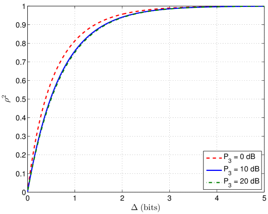
Figure 6: Variation of $\rho^{2}$ as a function of the gap $\Delta$ in bits. $b=1.5$.

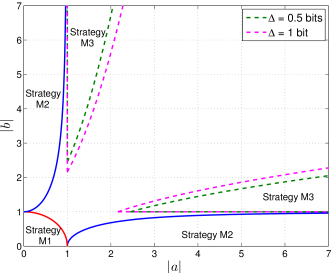
Figure 7: A plot of the channel conditions in Table V for a $3\times 3$ many-to-one XC for the three strategies. $P_{1}=P_{2}=P_{3}=0$ dB.

In Fig. 7 and Fig. 8, we plot the sub region in (24) for the sum-rate optimality of strategy $\small\mathcal{M}3$ as a graph in the $|a|\!-\!|b|$ plane for various values of $\Delta$, along with the sub-regions in Table V for strategies $\small\mathcal{M}1$ and $\small\mathcal{M}2$. We assume $P_{1}=P_{2}=P_{3}=0$ dB. As mentioned above, the sub-region in (24) shrinks for increasing values of $\Delta$.

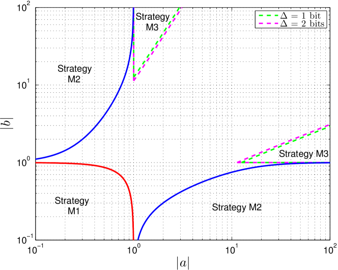
Figure 8: A plot of the channel conditions in Table V for a $3\times 3$ many-to-one XC for the three strategies. $P_{1}=P_{2}=P_{3}=10$ dB.

Strategy	Channel conditions
$\normalsize\mathcal{MI}1$	$a^{2}+b^{2}\leq 1$
$\normalsize\mathcal{MI}2$	(i) $a^{2}\geq 1+P_{1}+b^{2}P_{3},\;\,b^{2}\leq 1$
	(ii) $b^{2}\geq 1+P_{1}+a^{2}P_{2},\;\,a^{2}\leq 1$
$\normalsize\mathcal{MI}3$	(i) $a^{2}\geq 1+P_{1}+b^{2}P_{3},\;\,b^{2}\geq 1+P_{1}$
	(ii) $b^{2}\geq 1+P_{1}+a^{2}P_{2},\;\,a^{2}\geq 1+P_{1}$

TABLE VI: Sum-rate capacity results for a $3\times 3$ many-to-one IC in Theorem 7.

In Fig. 9, we plot the characterization of sum-rate capacity for the Gaussian many-to-one IC obtained in Theorem 8 for a $3\times 3$ many-to-one IC. Also plotted are the channel conditions determined in Theorem 7 for strategies $\mathcal{MI}1$, $\mathcal{MI}2$, and $\mathcal{MI}3$ to achieve sum-rate capacity. For $K=3$, and using same notation as in many-to-one XC with $a=h_{2}$, $b=h_{3}$, sub-region (56) becomes

1. $a^{2}\;\leq\;(1+b^{2}P_{3})\left(\displaystyle 1+\frac{1}{P_{2}}\right);\quad b^{2}\leq 1$

2. $b^{2}\;\leq\;(1+a^{2}P_{2})\left(\displaystyle 1+\frac{1}{P_{3}}\right);\quad a^{2}\leq 1$.

The above region is illustrated in the figure for $P_{1}=P_{2}=P_{3}=3$ dB. As mentioned earlier, for $K=3$, the total gap between the sum-rate of strategy $\mathcal{MI}1$ and the sum-rate capacity of the $3\times 3$ many-to-one IC is less than one bit. Thus, as long as the channel coefficients lie within this region, the sum-rate capacity can be characterized to within one bit. The channel conditions in (52) and (53) in Theorem 7 for $K=3$ are summarized in Table VI. The sum-rate capacity in the low-interference regime, i.e., strategy $\mathcal{MI}1$ was proved in [7].

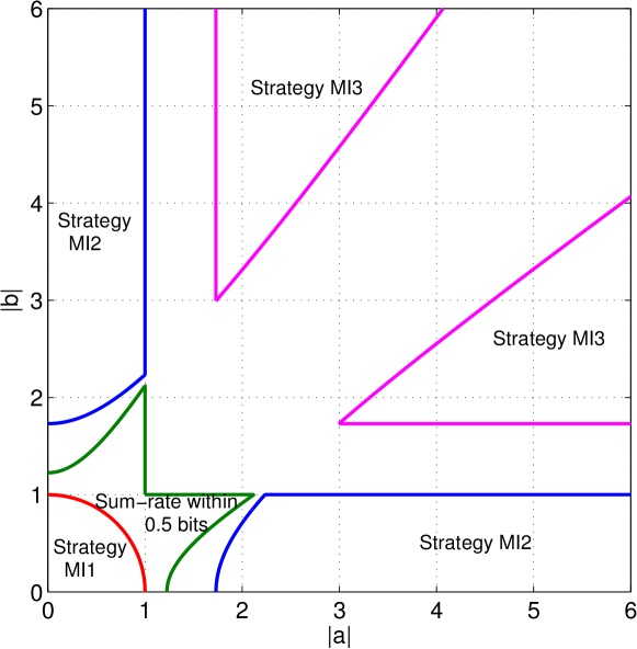
Figure 9: A plot of the channel conditions in Theorem 7 (summarized in Table VI) and Theorem 8 for a $3\times 3$ many-to-one IC. $P_{1}=P_{2}=P_{3}=3$ dB.

VII Conclusions

We considered the Gaussian many-to-one X channel with messages on all the links. We formulated different transmission strategies and obtained sufficient channel conditions under which the strategies were either optimal or within a gap from an outer bound. In the process, sum-rate capacity was characterized in some sub-regions of the many-to-one X channel. Subsequently, we identified a region in which the many-to-one X channel can be operated as a many-to-one interference channel without loss of sum-rate and further showed that in this region, the sum-rate capacity can be characterized to within a constant number of bits. We next formulated transmission strategies for the Gaussian many-to-one interference channel and obtained channel conditions under which the strategies achieved sum-rate capacity. We also identified a region where sum-rate capacity can be characterized to within a constant number of bits. This region is larger than the region implied by the corresponding result for the Gaussian many-to-one X channel.

We have restricted ourselves to the Gaussian many-to-one XC, since it is much harder to obtain exact sum-rate capacity results for the general fully connected $K\times K$ XC. The main difficulty lies in proving the decodability of intended message sets at the receivers for the various transmission strategies. For example, in case of the $K\times K$ many-to-one XC in standard form, we made use of Lemma 1 to show that under certain channel conditions, $y_{1}$ is a degraded version of $y_{i}$ with respect to message $W_{1i}$ and hence $H(W_{1i},W_{ii}\,|\,{\bf y}_{i}^{n})\leq 2n\epsilon_{n}$. We subsequently made use of this result in Theorem 1 to prove the sum-rate optimality of strategy $\mathcal{M}1$, which involves using Gaussian codebooks and treating interference as noise. However, extending this result to the general $K\times K$ XC is not easy. It is not clear if identification of a smart genie is possible for this setting. In [17, 18], it has been shown that treating interference as noise (strategy $\mathcal{M}1$ in this paper) is optimal for the $K\times K$ XC for the sum-rate capacity up to a constant gap. It would be interesting to study the applicability of techniques used in [17, 18] to analyze strategy $\mathcal{M}2$.

References

• [1] A. B. Carleial, “Interference channels,” IEEE Trans. Inform. Theory, vol. IT-24, pp. 60–70, Jul. 1978.
• [2] T. Han and K. Kobayashi, “A new achievable rate region for the interference channel,” IEEE Trans. Inform. Theory, vol. 27, no. 1, pp. 49–60, Jan. 1981.
• [3] G. Kramer, “Outer bounds on the capacity of Gaussian interference channels,” IEEE Trans. Inform. Theory, vol. 50, no. 3, pp. 581–586, Mar. 2004.
• [4] R. H. Etkin, D. N. C. Tse, and H. Wang, “Gaussian interference channel capacity to within one bit,” IEEE Trans. Inform. Theory, vol. 54, no. 12, pp. 5534–5562, Dec. 2008.
• [5] X. Shang, G. Kramer, and B. Chen, “A new outer bound and the noisy-interference sum-rate capacity for the Gaussian interference channels,” IEEE Trans. Inform. Theory, vol. 55, no. 2, pp. 689–699, Feb. 2009.
• [6] A. S. Motahari and A. K. Khandani, “Capacity bounds for the Gaussian interference channel,” IEEE Trans. Inform. Theory, vol. 55, no. 2, pp. 620–643, Feb. 2009.
• [7] V. S. Annapureddy and V. Veeravalli, “Gaussian interference networks: sum capacity in the low-interference regime and new outer bounds on the capacity region,” IEEE Trans. Inform. Theory, vol. 55, no. 7, pp. 3032–3050, Jul. 2009.
• [8] O. Koyluoglu, M. Shahmohammadi, and H. El Gamal, “A new achievable rate region for the discrete memoryless X channel,” Proc. IEEE ISIT’2009, pp. 2427–2431, Jul. 2009.
• [9] C. Huang, S. A. Jafar, and V. R. Cadambe, “Interference alignment and the generalized degrees of freedom of the X channel,” IEEE Trans. Inform. Theory, vol. 58, no. 8, pp. 5130–5150, Aug. 2012.
• [10] V. R. Cadambe and S. A. Jafar, “Interference alignment and a noisy interference regime for many-to-one interference channels,” e-print arXiv:0912.3029 [cs.IT], Dec. 2009. [Online]. http://arxiv.org/pdf/0912.3029.pdf
• [11] G. Bresler, A. Parekh, and D.  Tse, “The approximate capacity of the many-to-one and one-to-many Gaussian interference channels,” IEEE Trans. Inform. Theory, vol. 56, no. 9, pp. 4566–4592, Sep. 2010.
• [12] A. Jovicic, H. Wang, and P. Viswanath, “On network interference management,” IEEE Trans. Inform. Theory, vol. 56, no. 10, pp. 4941–4955, Oct. 2010.
• [13] B. Muthuramalingam, S. Bhashyam, and A. Thangaraj, “A decode and forward protocol for two-stage Gaussian relay networks,” IEEE Trans. on Comm., vol. 60, no. 1, pp. 68–73, Jan. 2012.
• [14] R. Prasad, S. Bhashyam, and A. Chockalingam, “Optimum transmission strategies for the one-to-many interference network,” in Proc. IEEE WCNC’2014, Istanbul, Turkey, Apr. 2014, pp. 12–17.
• [15] F. Zhu, X. Shang, B. Chen, and H. V. Poor, “On the capacity of multiple-access-Z-interference channels,” IEEE Trans. Inform. Theory, vol. 60, no. 12, pp. 7732–7750, Dec. 2014.
• [16] C. Geng, N. Naderializadeh, A. Avestimeher, and S. A. Jafar, “On the optimality of treating interference as noise,” IEEE Trans. Inform. Theory, vol. 61, no. 4, pp. 1753–1767, Apr. 2015.
• [17] C. Geng, H. Sun, and S. A. Jafar, “On the optimality of treating interference as noise: general message sets,” in Proc. IEEE ISIT’2014, Honolulu, USA, Jul. 2014, pp. 1777–1781.
• [18] C. Geng, H. Sun, and S. A. Jafar, “On the optimality of treating interference as noise: general message sets,” e-print arXiv:1401.2592 [cs.IT], Jan 2014, [Online]. http://arxiv.org/pdf/1401.2592v1.pdf
• [19] U. Niesen and M. Maddah-Ali, “Interference alignment: from degrees of freedom to constant-gap capacity approximations,” IEEE Trans. Inform. Theory, vol. 59, no. 8, pp. 4855–4888, Aug. 2013.
• [20] N. Liu and S. Ulukus, “On the capacity region of the Gaussian Z-channel,” in Proc. IEEE GLOBECOM’2004, vol. 1, Texas, USA, Dec. 2004, pp. 415–419.
• [21] H. F. Chong, M. Motani, and H. K. Garg, “Capacity theorems for the “Z” channel,” IEEE Trans. Inform. Theory, vol. 53, no. 4, pp. 1348–1365, Apr. 2007.
• [22] X. Shang, G. Kramer, and B. Chen, “New outer bounds on the capacity region of Gaussian interference channels,” in Proc. IEEE ISIT’2008, Toronto, Canada, Jul. 2008, pp. 245–249.
• [23] T. Liu and P. Viswanath, “An extremal inequality motivated by multiterminal information-theoretic problems,” IEEE Trans. Inform. Theory, vol. 53, no. 5, pp. 1839–1851, May 2007.