Modeling and Estimation of the Humans’ Effect on the CO₂ Dynamics Inside a Conference Room

Abstract

We develop a data-driven, Partial Differential Equation-Ordinary Differential Equation (PDE-ODE) model that describes the response of the Carbon Dioxide (CO₂) dynamics inside a conference room, due to the presence of humans, or of a user-controlled exogenous source of CO₂. We conduct two controlled experiments in order to develop and tune a model whose output matches the measured output concentration of CO₂ inside the room, when known inputs are applied to the model. In the first experiment, a controlled amount of CO₂ gas is released inside the room from a regulated supply, and in the second, a known number of humans produce a certain amount of CO₂ inside the room. For the estimation of the exogenous inputs, we design an observer, based on our model, using measurements of CO₂ concentrations at two locations inside the room. Parameter identifiers are also designed, based on our model, for the online estimation of the parameters of the model. We perform several simulation studies for the illustration of our designs.

1 Introduction

1.1 Motivation

Reducing energy demand is an important component of smart building research. Building energy use is responsible for an increasing proportion of the total energy demand. In the United States, the proportion of building electricity consumption has raised to 40% in 2005, from 33% in 1980 [19] and in Singapore, buildings accounted for 31% of the total electricity consumption for the year 2007 [38]. Thus, the problem of reducing building energy demand through advanced technologies and finer-tuned services has been the focus of ongoing research. The knowledge of occupancy levels in discrete zones within a building offers the potential of significant energy savings when coupled with zonal control of building services [1, 15, 20], which is a motivation for the work presented in the present article.

A relatively unexplored approach for estimating the number of humans occupying discrete zones of office spaces, such as, for example, a conference room within a larger office space, is to model and estimate the effect of the CO₂ that is produced from humans on the total CO₂ concentration in the specific discrete zone (i.e., the conference room). The reason is that humans are the primary producers of CO₂ inside a building [41] and that CO₂ sensors are widely deployed in smart buildings (since CO₂ is an important quantity to observe in order to manage occupant comfort [41] and since this quantity can be measured using sensors which are cheap).

Modeling CO₂ dynamics is challenging, due to the complexity of air dynamics. Most recently, two categories of models are used: Zonal models and Computational Fluid Dynamics (CFD) models. CFD models provide the most rich and detailed view of air motion in a space, however, they are beset by arduous work in modeling the physical space (e.g. providing locations of all walls, furniture, and occupants) and identifying all parameters that are needed for the model. CFD models also suffer from lengthy computation times to solve the necessary PDEs at a high resolution, especially near boundaries [32], [40]. Zonal models relate the movement of air between discrete and well-mixed spaces, such as rooms and parts of rooms. Generally, zonal models rely on ODE mass-balance laws between these spaces, which, in comparison to CFD models, can be solved very quickly [32]. However, this comes at the expense of not modeling the distributed nature of airborne contaminant transfer within a single space, and complex local phenomena such as jets of air coming from a vent [33].

Yet, for designing and implementing estimation algorithms for the CO₂ concentration, one has to develop a simple, and at the same time, accurate PDE-based model that retains the distributed character of the system. Based on this model, one can then design an observer for estimating the unknown CO₂ input that is produced from humans. The observer design has to be developed using the minimum number of sensors, in order to reduce cost and increase reliability. It is also crucial to develop online identifiers for the parameters of the model, since these parameters change with time due to their dependency on time-varying quantities such as heat generation [4].

1.2 Literature

Boundary observers for some classes of PDEs are constructed in [17], [18], [25], [26], [44] via backstepping. In [35], this methodology is applied for the estimation of the state-of-charge of batteries. Observer designs for time-delay systems with unknown inputs are presented in [2], [5], [23]. Swapping identifiers, originally developed for parameter estimation of ODE systems [21], [24], are constructed for parabolic PDEs in [43], [45], [46], [47]. In [34] this class of identifiers is employed for the identification of the state-of-health of batteries. Update laws for the estimation of unknown plant parameters and delays, in adaptive control of linear and nonlinear systems with input delays, are developed in [7], [8], [10], [11], [12], [13].

1.3 Results

We model the dynamics of the CO₂ concentration in the room using a convection PDE with a source term which is the output of a first-order ODE system driven by an unknown input which models the human’s emission rate of CO₂. The source term represents the effect of the humans on the CO₂ concentration in the room. In our experiments, we observe a delay in the response of the CO₂ concentration in the room to changes in the human’s input. For this reason, the source term is a filtered version of the unknown input rather than the actual input. We assume that the unmeasured input from the humans has the form of a piecewise constant signal. This formulation is based on our experimental observation that humans contribute to the rate of change of the CO₂ concentration of the room with a filtered version of step-like changes in the rate of CO₂.

The value of the PDE at the one boundary of its spatial domain indicates the CO₂ concentration inside the room at the location of the air supply. At this location, incoming air is entering the room, and hence, one can view the CO₂ concentration of the fresh incoming air as an input to the system. The value of the PDE at the other boundary of its spatial domain indicates the CO₂ concentration at the air return of the ventilation system. The air at this point is mixed with CO₂ that convects from the air supply towards the air return, and with CO₂ that is produced from humans. We consider the CO₂ concentration at this point as the output of our system. Any value of the PDE on an interior point of its spatial domain is an indicator of the concentration of CO₂ at the ceiling in a (non-ratiometric) normalized distance along an axis from the supply to the return vent.

We design an observer for the overall PDE-ODE system using boundary measurements (at the air supply and the air return). The observer estimates the unknown input from the humans, as well as the overall PDE state of our model. Our observer design and the proof of exponential stability of the observation error is based on the observer design from [6] for linear systems with distributed sensor delays. We design PDE and ODE swapping identifiers for the three constant parameters of the overall PDE-ODE system, namely the convection speed of the PDE, the coefficient that multiplies the source term which affects the PDE state on its whole spatial domain, and the time constant of the ODE. We prove that all the identifiers are stable and that the identifier of the time constant of the ODE converge to its true value when the input from the humans is not zero. For the case in which the convection speed is known, we also prove that both the identifiers for the coefficient that multiplies the source term in the PDE and the time constant of the ODE converge to their true vales when the input from the humans is not zero.

1.4 Structure of the Article

In Section 2, we derive a coupled PDE-ODE model for the dynamics of the CO₂ concentration in the room. In Section 3, we design an observer for the estimation of the total CO₂ that is generated by humans. We design parameter identifiers in Section 4, which are used for online estimation of the values of the model’s parameters.

Notation: The spatial $L_{2}(0,1)$ norm is denoted by $\|\cdot\|$. The temporal norms are denoted by $\mathcal{L}_{\infty}$ and $\mathcal{L}_{2}$ for $t\geq 0$.

2 Model of the CO₂ Dynamics

Our model consists of a PDE and an ODE part. The ODE part is given by

$$\dot{X}(t) = -aX(t)+V(t)$$ (1)

$$\dot{V}(t) = 0,$$ (2)

where, $X(t)$, in ppm, models the source term of human CO₂ production on the relative concentration (in ppm) of the room in the local vicinity of the human (the evolution of which is described later on by a PDE), and $V(t)$ is a step-valued function, in ppm $\cdot$ s^-1, representing the level of the human CO₂ production rate within the vicinity of humans. Parameter, $\frac{1}{a}$, in units of $100$s, represents a time constant specifying how fast changes in occupancy affect the CO₂ concentration in the room, in the local vicinity of the human.

The ODE is coupled with a PDE that models the CO₂ concentration in the room given by

$$u_{t}(x,t) = bu_{x}(x,t)+b_{X}X(t)$$ (3)

$$u(0,t) = U_{\rm e}-\Delta U(t),$$ (4)

with $\Delta U(t)=U(t)-U_{\rm e}$, where $u(x,t)$, in ppm, is the concentration of CO₂ in the room at a time $t\geq 0$ s and for $0\leq x\leq 1$, $-b>0$, in $\frac{1}{100\textrm{s}}$, represents the rate of air movement in the room, and $b_{X}>0$, in $\frac{1}{10^{4}\textrm{s}}$, specifies the rate of diffusion of CO₂ from the local vicinity of the human to the room. The spatial variable $x$ is unitless and represents a normalized distance along a horizontal axis that connects the air supply and air return. The air supply and air return are located at $x=0$ and $x=1$ respectively. Therefore, $u(0,t)$ is the CO₂ concentration inside the room at the location of the air supply and $u(1,t)$ is the CO₂ concentration inside the room at the location of the air return. The input $U(t)$ is the measured $\mathrm{p}\mathrm{p}\mathrm{m}$ concentration of the fresh incoming air. We do not simply specify the boundary condition at $x=0$ as $u(0,t)=U(t)$. The reason is that during our experiments we observe that a sudden drop in the measured CO₂ concentration at the air supply results in an increase of the CO₂ concentration at the air return. Our explanation for this effect is that a drop in CO₂ concentration at the supply from its equilibrium value corresponds to increased airflow at the vent, i.e. more fresh air gets mixed in the local vicinity. The increased airflow has the effect of pushing pockets of CO₂ air out of the return vent. One way to capture this effect is to multiply the difference of the CO₂ concentration from its equilibrium value $\Delta U(t)=U(t)-U_{\rm e}$ with minus one, where $U_{\rm e}$, in ppm, is the steady state input CO₂ concentration at the supply ventilation.

In Fig. 1,

\begin{overpic}[width=260.17464pt,tics=5]{PDEdrawing.eps} \put(32.0,15.0){Input from humans} \put(29.0,60.0){Direction of convection} \put(29.0,57.0){} \put(85.0,73.0){Supply} \put(2.0,73.0){Return} \put(47.0,10.0){$V$} \put(44.0,49.0){$u(x,t)$} \put(5.0,36.0){$u(1,t)$} \put(86.0,36.0){$u(0,t)$} \put(86.0,26.0){$X$} \put(3.0,60.0){$u(1,t)$} \put(88.0,60.0){$U(t)$} \end{overpic}

Figure 1: The geometrical representation of our model. Fresh air ($U$) enters the room from the supply ventilation. Air near the ceiling ($u$) convects from the air supply to the air return vent. The humans produce CO₂ ($V$) which rises ($X$) to the ceiling.

we illustrate the geometrical representation of our model. The PDE portion of the model, $u(x,t)$, represents convection of air from the air supply to the air return vent near the ceiling. Note the absence of a diffusive term, which we have omitted since it plays a relatively minor role in dispersing indoor pollutants [4]. We choose to model the CO₂ concentrations near the ceiling since this is where we see most effect from human-generated CO₂ . This is explained by the fact that a warm breath from a human occupant acts as a “bubble” of gas that rises to the ceiling, since it is more buoyant than the ambient, cooler air. Thus, the air coming from lower in the room is modeled as a source term on the PDE across its entire length. The ODE portion of the model is intended to model the fact that this bubble of air does not immediately rise to the ceiling but only gradually.

In Fig. 2

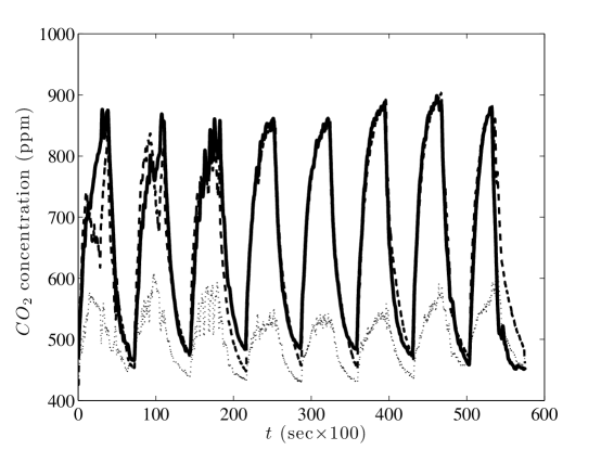
Figure 2: Solid line: The simulated concentration of CO₂ at the air return $u(1,t)$ given by the model (1)–(4) for Experiment I. Dashed line: The concentration of the CO₂ at the air return measured by the CO₂ sensor. Dotted line: The concentration of CO₂ at the air supply measured by the CO₂ sensor.

we show the concentration of CO₂ at the air return and the air supply measured by the CO₂ sensors for our first experiment in which we periodically release CO₂ every one hour. We also show the output $u(1,t)$ of our model with parameters as shown in Table 1 and initial condition $u(x,0)=400$ ppm.

Table 1: Parameters of the Model (1)–(4) for Experiment I.

Physical Paramater	Model parameter	Value
Convection coefficient $\left(\frac{1}{100\rm{s}}\right)$	$-b$	$0.8$
Source term coefficient $\left(\frac{1}{10^{4}\rm{s}}\right)$	$b_{X}$	$0.2$
Time constant of the human’s effect $\left({100\rm{s}}\right)$	$\frac{1}{a}$	$10$
Equilibrium concentration at the air return (ppm)	$U_{\rm e}$	$450$

The input $V$ to our model, with which we emulate the behavior of the CO₂ that is released from the pump, is the square wave that is shown in Fig. 3.

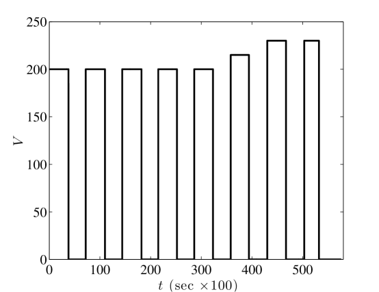
Figure 3: The input $V$ to the model (1)–(4) from Experiment I modeling the concentration of CO₂ that is released from the pump. When $V=0$ the CO₂ pump is turned off and when $V\neq 0$ the CO₂ pump is turned on.

In Fig. 4 we show the CO₂ concentration from Experiment II measured from the CO₂ sensor and predicted from model (1)–(4) with parameters shown in Table 2, initial condition $u(x,0)=400$ ppm, and input $V$ that is shown in Fig. 5, with which we emulate the behavior of the CO₂ that is produced by humans.

Table 2: Parameters of the Model (1)–(4) for Experiment II.

Physical Paramater	Model parameter	Value
Convection coefficient $\left(\frac{1}{100\rm{s}}\right)$	$-b$	$0.8$
Source term coefficient $\left(\frac{1}{10^{4}\rm{s}}\right)$	$b_{X}$	$0.16$
Time constant of the human’s effect $\left({100\rm{s}}\right)$	$\frac{1}{a}$	$10$
Equilibrium concentration at the air return (ppm)	$U_{\rm e}$	$370$

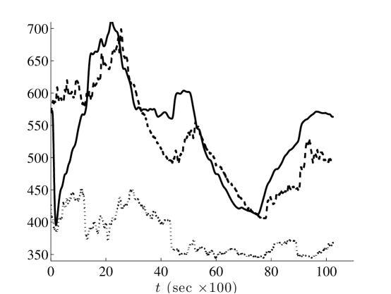
Figure 4: Solid line: The simulated concentration of the CO₂ at the air return $u(1,t)$ given by the model (1)–(4) for Experiment II. Dashed line: The concentration of the CO₂ at the air return measured by the CO₂ sensor. Dotted line: The concentration of CO₂ at the air supply measured by the CO₂ sensor.

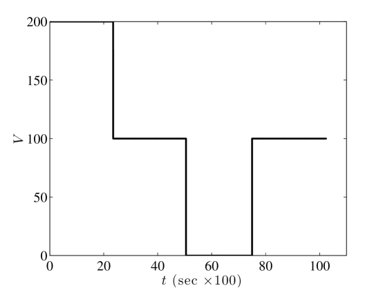
Figure 5: The input $V$ to the model (1)–(4) from Experiment II modeling the input concentration of CO₂ from the humans.

3 Estimation of the Humans’ Effect

We construct an observer for the plant (1)–(4) assuming measurements of $u(1,t)$ and $U(t)$. We assume that the parameters of the model are known, since they can either be manually identified (as in Section 2), or they can be identified using parameter identifiers (as in Section 4).

3.1 Observer Design

We consider the following observer which is a copy of the plant plus output injection

$$\hat{u}_{t}(x,t) = b\hat{u}_{x}(x,t)+b_{X}\hat{X}(t)+p(x)\left(u(1,t)-\hat{u}(1,t)\right)$$ (5)

$$\hat{u}(0,t) = -U(t)+2U_{\rm e}$$ (6)

$$\dot{\hat{X}}(t) = -a\hat{X}(t)+\hat{V}(t)+L_{1}\left(u(1,t)-\hat{u}(1,t)\right)$$ (7)

$$\dot{\hat{V}}(t) = L_{2}\left(u(1,t)-\hat{u}(1,t)\right).$$ (8)

The following corollary is a consequence of Theorem 2 in [6].

Corollary 1

Consider the system (1)–(4) and the observer (5)–(8) with

$$p(x) = L_{1}\gamma_{1}(x)+L_{2}\gamma_{2}(x)$$ (9)

$$\gamma_{1}(x) = \frac{b_{X}}{a}\left(e^{-\frac{a}{b}x}-1\right)$$ (10)

$$\gamma_{2}(x) = -\frac{b_{X}}{ba}x+\frac{b_{X}}{a^{2}}\left(1-e^{-\frac{a}{b}x}\right).$$ (11)

Let $b_{X}\neq 0$ and choose $L_{1}$, $L_{2}$ such that the matrix $A-\left[\begin{array}[]{ll}L_{1}\\ L_{2}\end{array}\right]C$, where

$$A = \left[\begin{array}[]{ll}-a&1\\ 0&0\end{array}\right]$$ (14)

$$C = \left[\begin{array}[]{ll}\gamma_{1}(1)&\gamma_{2}(1)\end{array}\right],$$ (16)

is Hurwitz. Then for any $u(x,0),\hat{u}(x,0)\in L_{2}(0,1)$, $X(0),\hat{X}(0),V(0),\hat{V}(0)\in\mathbb{R}$, there exist positive constants $\kappa$ and $\lambda$ such that the following holds for all $t\geq 0$

$$\Omega(t) \leq \kappa\Omega(0)e^{-\lambda t}$$ (17)

$$\Omega(t) = \int_{0}^{1}\left(u(x,t)-\hat{u}(x,t)\right)^{2}dx+\left(X(t)-\hat{X}(t)\right)^{2}+\left(V(t)-\hat{V}(t)\right)^{2}.$$ (18)

Proof 1

It is sufficient to show that if $b_{X}\neq 0$ then the pair $\left(A,C\right)$ is observable (in which case one can choose $L_{1}$ and $L_{2}$ such that the matrix $A-\left[\begin{array}[]{ll}L_{1}\\ L_{2}\end{array}\right]C$ is Hurwitz), which allow one to then use Theorem 2 in [6]. The determinant of the observability matrix $O$ of the pair $(A,C)$ is $\textrm{det}(O)=\gamma_{1}(1)\left(\gamma_{1}(1)+a\gamma_{2}(1)\right)$. Using (10), (11) it follows that $\rm{det}\neq 0$ whenever $b_{X}\neq 0$.

4 Online Parameter Identification

We design swapping identifiers (see [21], [24] for the case of ODEs and [34], [43] for the case of parabolic PDEs) for online identification of the parameters $b$, $b_{X}$ and $a$. We now assume that the ODE and PDE states are measured. Directly measuring these quantities in an actual implementation might be impractical. Yet, our online parameter identifiers can be in principle combined with a state-estimation algorithm in order to simultaneously perform state estimation and parameter identification, i.e., in order to design an adaptive observer (although, as it is discussed in Section 5, for PDE systems this is highly nontrivial and there is no systematic approach for such a design).

4.1 Identifier Design

We deal first with the identification of $b$ and $b_{X}$. Define the “estimation” error

$$e(x,t)=u(x,t)-bv(x,t)-b_{X}p(x,t)-\eta(x,t),$$ (19)

between the measured state $u$ and the signals $v$, $p$, $\eta$, where $v$ is a filter for $u_{x}$, $p$ a filter for $X$ and $\eta$ is an input filter, given by

$$v_{t}(x,t) = \hat{b}v_{x}(x,t)+u_{x}(x,t)$$ (20)

$$v(0,t) = 0$$ (21)

$$p_{t}(x,t) = \hat{b}p_{x}(x,t)+X(t)$$ (22)

$$p(0,t) = 0$$ (23)

$$\eta_{t}(x,t) = \hat{b}\eta_{x}(x,t)-\hat{b}u_{x}(x,t)$$ (24)

$$\eta(0,t) = -U(t)+2U_{e}.$$ (25)

The goal of the filters (20)–(25) is to convert the dynamic parametrization of the plant into a static one. This is the main attribute of the swapping identification method [21], [24], [43]. Using the static relationship (19) as a parametric model and defining the “prediction error”

$$\hat{e}(x,t)=u(x,t)-\hat{b}v(x,t)-\hat{b}_{X}p(x,t)-\eta(x,t),$$ (26)

the identifiers for $b$ and $b_{X}$ are given by the following gradient update laws with normalization

$$\dot{\hat{b}}(t) = -\gamma_{1}\hat{b}(t)\textrm{Proj}_{\bar{b}}\left\{\frac{\int_{0}^{1}\hat{e}(x,t)v(x,t)dx}{1+\int_{0}^{1}v(x,t)^{2}dx+\int_{0}^{1}p(x,t)^{2}dx}\right\}$$ (27)

$$\dot{\hat{b}}_{X}(t) = -\gamma_{2}\hat{b}(t)\frac{\int_{0}^{1}\hat{e}(x,t)p(x,t)dx}{1+\int_{0}^{1}v(x,t)^{2}dx+\int_{0}^{1}p(x,t)^{2}dx},$$ (28)

where the projector operator is defined as

$$\mbox{Proj}_{\bar{b}}\{\tau\} = \left\{\begin{array}[]{cc}0,&\mbox{if $\hat{b}=\bar{b}$ and $\tau>0$}\\ \tau,&\mbox{otherwise}\end{array}\right..$$ (31)

and $\gamma_{1},\gamma_{2}>0$, $\bar{b}<0$. The goal of the projection operator is to ensure that $\hat{b}<\bar{b}$. We design next an online identifier for $a$. Define the filters

$$\dot{\Omega}_{0}(t) = \bar{A}\left(\Omega_{0}(t)-X(t)\right)+V(t)$$ (32)

$$\dot{\Omega}(t) = \bar{A}\Omega(t)-X(t),$$ (33)

where $\bar{A}<0$. Defining the error

$$\epsilon(t)=X(t)-\Omega_{0}(t)-\Omega(t){a},$$ (34)

the identifier for $a$ is

$$\dot{\hat{a}}(t) = \gamma_{3}\frac{\hat{\epsilon}(t)\Omega(t)}{1+\Omega(t)^{2}}$$ (35)

$$\hat{\epsilon}(t) = X(t)-\Omega_{0}(t)-\Omega(t)\hat{a}(t),$$ (36)

where $\gamma_{3}>0$. Defining the estimation error of a parameter $m$ as

$$\tilde{m}=m-\hat{m},$$ (37)

the following can be proved.

Theorem 1

Consider system (1)–(4) with the update laws (20)–(31), (32), (33), (35), (36), and let $b<\bar{b}$, where $\bar{b}$ is known. Then for all $V(0)$, $X(0)$, $\hat{b}(0)$, $\hat{b}_{X}(0)$, $\hat{a}(0)$, $\Omega(0)$, $\Omega_{0}(0)$, $\in\mathbb{R}$, $v(x,0)$, $p(x,0)$, $\eta(x,0)$ $\in L_{2}(0,1)$, $u(x,0)\in H_{1}(0,1)$, and $U,\dot{U}\in\mathcal{L}_{\infty}$,

$$\|u_{x}\|,\|u\|,V,X,\|v\|,\|p\|,\|\eta\|,\Omega,\Omega_{0},\tilde{b},\tilde{b}_{X},\tilde{a}\in\mathcal{L}_{\infty},$$ (38)

$$\dot{\hat{b}},\dot{\hat{b}}_{X},\dot{\hat{a}},\frac{\|\hat{e}\|}{\sqrt{1+\|v\|^{2}+\|p\|^{2}}},\frac{|\hat{\epsilon}|}{\sqrt{1+\Omega^{2}}}\in\mathcal{L}_{2}\cap\mathcal{L}_{\infty}.$$ (39)

Moreover, if $\lim_{t\to\infty}V(t)\to c$, with $c\neq 0$, then $\lim_{t\to\infty}\hat{a}(t)\to a$.

Proof 2

See Appendix A.

In the special case in which $b$ is known, one does not need to design an update law for $b$ and the following can be proved.

Lemma 1

Let $b$ be known. Consider the update law for $a$ given by (35) and the update law for $b_{X}$ given by

$$\dot{\hat{b}}_{X}(t) = \gamma\frac{\int_{0}^{1}\hat{\zeta}(x,t)\mu(x,t)dx}{1+\int_{0}^{1}\mu(x,t)^{2}dx},$$ (40)

where

$$\hat{\zeta}(x,t) = u(x,t)-\hat{b}_{X}\mu(x,t)-\xi(x,t)$$ (41)

$$\mu_{t}(x,t) = b\mu_{x}(x,t)+X(t)$$ (42)

$$\mu(0,t) = 0$$ (43)

$$\xi_{t}(x,t) = b\xi_{x}(x,t)$$ (44)

$$\xi(0,t) = -U(t)+2U_{e}.$$ (45)

Then for all $V(0)$, $X(0)$, $\hat{b}_{X}(0)$, $\hat{a}(0)$, $\Omega(0)$, $\Omega_{0}(0)$, $\in\mathbb{R}$, $u(x,0)$, $\mu(x,0)$, $\xi(x,0)$ $\in L_{2}(0,1)$, and $U\in\mathcal{L}_{\infty}$,

$$\|u\|,V,X,\|\mu\|,\|\xi\|,\Omega,\Omega_{0},\tilde{b}_{X},\tilde{a}\in\mathcal{L}_{\infty},\quad\mbox{and}\quad\dot{\hat{b}}_{X},\dot{\hat{a}}\in\mathcal{L}_{2}\cap\mathcal{L}_{\infty},$$ (46)

$$\frac{\|\hat{\zeta}\|}{\sqrt{1+\|\mu\|^{2}}},\frac{|\hat{\epsilon}|}{\sqrt{1+\Omega^{2}}}\in\mathcal{L}_{2}\cap\mathcal{L}_{\infty}.$$ (47)

Moreover, if $V(0)=c$ with $c\neq 0$, then $\lim_{t\to\infty}\hat{b}_{X}(t)\to b_{X}$ and $\lim_{t\to\infty}\hat{a}(t)\to a$.

Proof 3

See Appendix B.

5 Conclusions

In this article, we develop a PDE-ODE model that describes the dynamics of the CO₂ concentration in a conference room. We validate our model by conducting two different experiments. We design and validate an observer for the estimation of the unknown CO₂ input that is generated by humans. We also design online parameter identifiers for the online estimation of the parameters of the model.

Future work will address the problem of estimation of the actual human occupancy level using measurements of CO₂. This is a highly nontrivial problem because humans’ CO₂ generation rates can vary widely between different persons depending on current activity, diet, and body size [40].

Another topic for future research is to combine the observer design with the update laws for the estimation of the parameters of the model. In other words, to design an adaptive observer [21]. Yet, in contrast to the finite-dimensional case, in the case of PDE systems this is far from trivial due to the lack of systematic procedures for the construction of state-transformations that can transform the original system to a system having an observer canonical form [21], [43]. For this reason designing adaptive observers for PDE systems is possible only in special cases [43]. As an alternative one could resort to finite-dimensional approximations as it is done, for example, in [36].

Appendix A

Proof of Theorem 1

Using (3), (4) together with (20), (25) one can show that the error (19) satisfies

$$e_{t}(x,t) = \hat{b}e_{x}(x,t)$$ (A.1)

$$e(0,t) = 0.$$ (A.2)

Analogously, using (1), along with (32), (33), it is shown that the error (34) satisfies

$$\dot{\epsilon}(t)=\bar{A}\epsilon(t).$$ (A.3)

Consider the Lyapunov function

$$V(t) = \int_{0}^{1}(2-x)e(x,t)^{2}dx+\frac{1}{2}\epsilon(t)^{2}+\frac{1}{2\gamma_{1}}\tilde{b}(t)^{2}+\frac{1}{2\gamma_{2}}\tilde{b}_{X}(t)^{2}$$ (A.4)

$$-\frac{\bar{A}}{2\gamma_{3}}\tilde{a}(t)^{2}.$$

Taking the derivative of $V$, using the fact that for a constant parameter $\dot{\tilde{m}}=-\dot{\hat{m}}$, the update laws (27), (28), (35), the properties of the projector operator (see for example [24]) and relations (A.1), (A.2), (A.3) we get that

$$\dot{V}(t) \leq \hat{b}(t)e(1,t)^{2}+\hat{b}(t)\int_{0}^{1}e(x,t)^{2}dx+\bar{A}\epsilon(t)^{2}+\hat{b}(t)\tilde{b}(t)$$ (A.5)

$$\times\frac{\int_{0}^{1}\hat{e}(x,t)v(x,t)dx}{1+\int_{0}^{1}v(x,t)^{2}dx+\int_{0}^{1}p(x,t)^{2}dx}+\hat{b}(t)\tilde{b}_{X}(t)$$

$$\times\frac{\int_{0}^{1}\hat{e}(x,t)p(x,t)dx}{1+\int_{0}^{1}v(x,t)^{2}dx+\int_{0}^{1}p(x,t)^{2}dx}+\bar{A}\tilde{a}(t)\frac{\hat{\epsilon}(t)\Omega(t)}{1+\Omega(t)^{2}}.$$

Using definitions (19), (26), and (34), (36) we get that

$$\hat{e}(x,t) = e(x,t)+\tilde{b}(t)v(x,t)+\tilde{b}_{X}(t)p(x,t)$$ (A.6)

$$\hat{\epsilon}(t) = \epsilon(t)+\tilde{a}(t)\Omega(t),$$ (A.7)

and hence,

$$\dot{V}(t) \leq \hat{b}(t)e(1,t)^{2}+\hat{b}(t)\int_{0}^{1}e(x,t)^{2}dx+\bar{A}\epsilon(t)^{2}$$ (A.8)

$$+\hat{b}(t)\frac{\int_{0}^{1}\hat{e}(x,t)^{2}dx-\int_{0}^{1}\hat{e}(x,t)e(x,t)dx}{1+\int_{0}^{1}v(x,t)^{2}dx+\int_{0}^{1}p(x,t)^{2}dx}-\bar{A}\frac{-\hat{\epsilon}(t)^{2}+\hat{\epsilon}(t)\epsilon(t)}{1+\Omega(t)^{2}}.$$

Using Young’s inequality and the fact that $\hat{b}(t)\leq\bar{b}<0$, for all $t\geq 0$, we arrive at

$$\dot{V}(t) \leq \bar{b}e(1,t)^{2}+\frac{\bar{b}}{2}\int_{0}^{1}e(x,t)^{2}dx+\frac{\bar{A}}{2}\epsilon(t)^{2}+$$ (A.9)

$$+\frac{\bar{b}}{2}\frac{\int_{0}^{1}\hat{e}(x,t)^{2}dx}{1+\int_{0}^{1}v(x,t)^{2}dx+\int_{0}^{1}p(x,t)^{2}dx}+\frac{\bar{A}}{2}\frac{\hat{\epsilon}(t)^{2}}{1+\Omega(t)^{2}}.$$

Using relation (A.9) we conclude that $\|e(t)\|$, $\epsilon$, $\tilde{b}$, $\tilde{b}_{X}$, $\tilde{a}$ are bounded, and that also $\frac{\sqrt{\int_{0}^{1}\hat{e}(x,t)^{2}dx}}{\sqrt{1+\int_{0}^{1}v(x,t)^{2}dx+\int_{0}^{1}p(x,t)^{2}dx}}$, $\frac{\left|\hat{\epsilon}(t)\right|}{\sqrt{1+\Omega(t)^{2}}}$ are square integrable. Therefore, using (27), (28), (35), and the boundness of $\tilde{b}$ (which implies also the boundness of $\hat{b}$) one can conclude that $\dot{\hat{b}}$, $\dot{\hat{b}}_{X}$, $\dot{\hat{a}}$ are square integrable, and using (A.6), (A.7) that $\frac{\|\hat{e}(t)\|}{\sqrt{1+\|v(t)\|^{2}+\|p(t)\|^{2}}}$ and $\frac{\left|\hat{\epsilon}(t)\right|}{\sqrt{1+\Omega(t)^{2}}}$ are bounded. Therefore, using the update laws (27), (28), (35) one can conclude that $\dot{\hat{b}}$, $\dot{\hat{b}}_{X}$, $\dot{\hat{a}}$ are also bounded. Using relations (1), (2), (32), (33) one can conclude that $V,X,\Omega,\Omega_{0}\in\mathcal{L}_{\infty}$. Using (3), (4) one can conclude that

$$u_{xt}(x,t) = bu_{xx}(x,t)$$ (A.10)

$$u_{x}(0,t) = -\frac{\dot{U}(t)+b_{X}X(t)}{b}.$$ (A.11)

With a Lyapunov functional as

$$V^{*}(t) = \int_{0}^{1}(2-x)u(x,t)^{2}dx+\int_{0}^{1}(2-x)u_{x}(x,t)^{2}dx$$ (A.12)

$$+\frac{b\bar{b}}{16}\int_{0}^{1}(2-x)v(x,t)^{2}dx+\int_{0}^{1}(2-x)p(x,t)^{2}dx,$$

we get along (3), (4), (A.10), (A.11), (20), (23), after using integration by parts and Young’s inequality that

$$\dot{V}^{*}(t) \leq \frac{b}{2}\int_{0}^{1}u(x,t)^{2}dx+\frac{b}{2}\int_{0}^{1}u_{x}(x,t)^{2}dx+\frac{\bar{b}}{2}\int_{0}^{1}v(x,t)^{2}dx$$ (A.13)

$$+\frac{\bar{b}}{2}\int_{0}^{1}p(x,t)^{2}dx-\frac{8}{\bar{b}}X(t)^{2}\left(b_{X}+1\right)-b\left(-U(t)+2U_{\rm e}\right)^{2}$$

$$-\frac{\left(\dot{U}(t)+b_{X}X(t)\right)^{2}}{\bar{b}},$$

and hence,

$$\dot{V}^{*}(t) \leq \frac{\bar{b}}{4}V^{*}(t)+M\left(X(t)^{2}+U(t)^{2}+\dot{U}(t)^{2}+U_{\rm e}^{2}\right),$$ (A.14)

where $M=-\frac{8}{\bar{b}}\left(b_{X}+1\right)-8b-2\frac{b_{X}^{2}+1}{\bar{b}}$. It follows since $U,X,\dot{U}\in\mathcal{L}_{\infty}$ that $\|u\|$, $\|u_{x}\|$, $\|v\|$, $\|p\|$, $\in\mathcal{L}_{\infty}$. Using (19) it follows that $\|\eta\|\in\mathcal{L}_{\infty}$.

We show next that $\lim_{t\to\infty}\tilde{a}(t)=0$ when $\lim_{t\to\infty}V(t)=c\neq 0$. Using (1), (33), and the fact that $a>0$, $\bar{A}<0$, one can conclude that $\Omega$ is bounded, when $V$ is bounded, with $\lim_{t\to\infty}\Omega(t)=\frac{c}{a\bar{A}}$, and hence, it is sufficient to show that $\lim_{t\to\infty}\hat{\epsilon}(t)=0$, since then, one can conclude using (A.3) and (A.7) that $\lim_{t\to\infty}\tilde{a}(t)=0$. Using an alternative to Barbalat’s Lemma from [30] it is sufficient to show that $\frac{dG(t)}{dt}$, where $G(t)=\frac{\hat{\epsilon}(t)^{2}}{{1+\Omega(t)^{2}}}$, is bounded. We have that $G$ satisfies the relation $\frac{dG(t)}{dt}=2\frac{\hat{\epsilon}(t)}{\sqrt{1+\Omega(t)^{2}}}\frac{\left(\bar{A}\epsilon(t)-\dot{\hat{a}}(t)\Omega(t)+\tilde{a}(t)\left(\bar{A}\Omega(t)-X(t)\right)\right)}{\sqrt{1+\Omega(t)^{2}}}-\frac{\hat{\epsilon}(t)^{2}}{1+\Omega(t)^{2}}\frac{\Omega(t)\left(\bar{A}\Omega(t)-X(t)\right)}{1+\Omega(t)^{2}}$. Since $\frac{\hat{\epsilon}(t)}{\sqrt{1+\Omega(t)^{2}}}$, $\epsilon$, $\dot{\hat{a}}$, $\tilde{a}$ are bounded, using (1) one can conclude that $X$ is also bounded (when $V$ is bounded), and hence, $\frac{dG(t)}{dt}$ is bounded.

Appendix B

Proof of Lemma 1

Using (3), (4) together with (42), (45) it is shown that for the error

$$\zeta(x,t) = u(x,t)-b_{X}\mu(x,t)-\xi(x,t),$$ (B.1)

it holds that

$$\zeta_{t}(x,t) = b\zeta_{x}(x,t)$$ (B.2)

$$\zeta(0,t) = 0.$$ (B.3)

Similarly to the proof of Theorem 1, using the fact that $\zeta(x,t)-\hat{\zeta}(x,t)=-\tilde{b}_{X}\mu(x,t)$, for the Lyapunov function

$$V(t) = -\frac{1}{b}\int_{0}^{1}(2-x)\zeta(x,t)^{2}dx+\frac{1}{2}\epsilon(t)^{2}+\frac{1}{2\gamma}\tilde{b}_{X}(t)^{2}-\frac{\bar{A}}{2\gamma_{3}}\tilde{a}(t)^{2},$$ (B.4)

along the solutions of (B.2), (B.3), (A.3), (40), (35) it holds that

$$\dot{V}(t) \leq -\zeta(1,t)^{2}-\frac{1}{2}\int_{0}^{1}\zeta(x,t)^{2}dx+\frac{\bar{A}}{2}\epsilon(t)^{2}-\frac{1}{2}\frac{\int_{0}^{1}\hat{\zeta}(x,t)^{2}dx}{1+\int_{0}^{1}\mu(x,t)^{2}dx}$$ (B.5)

$$+\frac{\bar{A}}{2}\frac{\hat{\epsilon}(t)^{2}}{1+\Omega(t)^{2}}.$$

We only prove that $\lim_{t\to\infty}b_{X}(t)\to b_{X}$. The rest of the lemma is proved using the same arguments with the proof of Theorem 1. Using (42), (43) it is shown that the variable $\bar{\mu}(x,t)=\mu(x,t)+\frac{c}{ab}x$ satisfies $\bar{\mu}_{t}(x,t)=b\bar{\mu}_{x}(x,t)+X(t)-\frac{c}{a}$, $\bar{\mu}(0,t)=0$. Using the fact that $V(0)=c$ we get from (1), (2) that $\tilde{X}(t)=e^{-at}\tilde{X}(0)$, where $\tilde{X}=X-\frac{c}{a}$. Therefore, $\tilde{X}\in\mathcal{L}_{2}$. For the function $V_{2}(t)=V_{1}(t)+\frac{9}{-2ab}\tilde{X}(t)^{2}$, where $V_{1}(t)=\int_{0}^{1}(2-x)\bar{\mu}(x,t)^{2}dx$ it holds that

$$\dot{V}_{2}(t)\leq\frac{b}{4}V_{1}(t)+\frac{1}{b}\tilde{X}(t)^{2}.$$ (B.6)

Therefore, $\sqrt{V_{1}}\in\mathcal{L}_{2}\cap\mathcal{L}_{\infty}$, and hence $\sqrt{\int_{0}^{1}\bar{\mu}(x,t)^{2}dx}\in\mathcal{L}_{2}$. Using the facts that $\int_{0}^{1}\hat{\zeta}(x,t)^{2}dx=\frac{\int_{0}^{1}\hat{\zeta}(x,t)^{2}dx}{1+\int_{0}^{1}\mu(x,t)^{2}dx}\left(1+\int_{0}^{1}\mu(x,t)^{2}dx\right)$, that $\sqrt{V_{1}}\in\mathcal{L}_{\infty}$, and that $\frac{\sqrt{\int_{0}^{1}\hat{\zeta}(x,t)^{2}dx}}{\sqrt{1+\int_{0}^{1}\mu(x,t)^{2}dx}}\in\mathcal{L}_{2}$, it also follows that $\sqrt{\int_{0}^{1}\hat{\zeta}(x,t)^{2}dx}\in\mathcal{L}_{2}$. Writing $\zeta(x,t)-\hat{\zeta}(x,t)+\tilde{b}_{X}\bar{\mu}(x,t)=\frac{c}{ab}x\tilde{b}_{X}$ we get that $\frac{c}{2ab}\left|\tilde{b}_{X}\right|\leq\sqrt{\int_{0}^{1}\zeta(x,t)^{2}dx}+\sqrt{\int_{0}^{1}\hat{\zeta}(x,t)^{2}dx}+\left|\tilde{b}_{X}\right|\sqrt{\int_{0}^{1}\bar{\mu}(x,t)^{2}dx}$, and hence, since also $\sqrt{\int_{0}^{1}\zeta(x,t)^{2}dx}\in\mathcal{L}_{2}$ and $\tilde{b}_{X}\in\mathcal{L}_{\infty}$, and $c\neq 0$ we get that $\tilde{b}_{X}\in\mathcal{L}_{2}$. Since $\tilde{b}_{X},\dot{\tilde{b}}_{X}\in\mathcal{L}_{\infty}$, one can conclude that $\frac{d\tilde{b}_{X}^{2}(t)}{dt}\in\mathcal{L}_{\infty}$, and hence, from the alternative to Barbalat’s Lemma from [30] we conclude that $\lim_{t\to\infty}\tilde{b}_{X}(t)\to 0$.

References

- [1] Y. Agarwal, B. Balaji, S. Dutta, R. K. Gupta, and T. Weng, “Duty-cycling buildings aggressively: The next frontier in HVAC control”, IEEE Conference on Information Processing in Sensor Networks, 2011.
- [2] S. Amin, X. Litrico, S. Sastry, and A. Bayen, “Cyber security of water SCADA systems: (II) Attack detection using enhanced hydrodynamic models,” IEEE Transactions on Control Systems Technology , vol. 21, pp. 1679–1693, 2012.
- [3] A. Bastani, F. Haghighat, J. A. Kozinski, “Contaminant source identification within a building: toward design of immune buildings,”, Building and Environment, vol. 51, pp. 320–329, 2012.
- [4] A. Baughman, A. Gadgil, and W. Nazaroff, “Mixing of a point source pollutant by natural convection flow within a room,” Indoor Air, vol. 4, pp. 114–122, 1994.
- [5] N. Bedjaoui, X. Litrico, D. Koenig, and P.O. Malaterre, “ observer for time-delay systems: Application to FDI for irrigation canal,” IEEE Conference on Decision and Control, San Diego, CA, 2006.
- [6] N. Bekiaris-Liberis and M. Krstic, “Lyapunov stability of linear predictor feedback for distributed input delays”, IEEE Transactions on Automatic Control, vol. 56, pp. 655–660, 2011.
- [7] N. Bekiaris-Liberis and M. Krstic, “Delay-adaptive feedback for linear feedforward systems,” Systems and Control Letters, vol. 59, pp. 277–283, 2010.
- [8] N. Bekiaris-Liberis, M. Jankovic, and M. Krstic, “Adaptive stabilization of LTI systems with distributed input delay,” International Journal of Adaptive Control and Signal Processing, vol. 27, pp. 46–65, 2013.
- [9] J. S. Bendat, A. G. Piersol, Engineering Applications of Correlation and Spectral Analysis, Wiley, 1980.
- [10] D. Bresch-Pietri and M. Krstic, “Delay-adaptive control for nonlinear systems,” IEEE Transactions on Automatic Control, in press, 2014.
- [11] D. Bresch-Pietri, J. Chauvin and N. Petit, “Adaptive control scheme for uncertain time-delay systems,” Automatica, vol. 48, pp. 1536–1552, 2012.
- [12] D. Bresch-Pietri and M. Krstic, “Delay-adaptive predictor feedback for systems with unknown long actuator delay,” IEEE Transactions on Automatic Control, vol. 55, pp. 2106–2112, 2010.
- [13] D. Bresch-Pietri and M. Krstic, “Adaptive trajectory tracking despite unknown input delay and plant parameters,” Automatica, vol. 45, pp. 2074–2081, 2009.
- [14] H. Cai, X. Li, Z. Chen, L. Kong, “Multiple indoor constant contaminant sources by ideal sensors: A Theoretical model and numerical validation,” Indoor and Built Environment, vol. 22, pp. 897–909, 2013.
- [15] C. Chao and J. Hu, “Development of a dual-mode demand control ventilation strategy for indoor air quality control and energy saving”, Building and Environment, vol. 39, pp. 385–397, 2004.
- [16] Q. Chen, “Ventilation performance prediction for buildings: A method overview and recent applications”, Building and Environment, vol. 44, pp. 848–858, 2009.
- [17] F. Di Meglio, R. Vazquez, and M. Krstic, “Stabilization of a system of coupled first-order hyperbolic linear PDEs with a single boundary input,” IEEE Transactions on Automatic Control, vol. 58, pp. 3097–3111, 2013.
- [18] F. Di Meglio, D. Bresch-Pietri and U. J. F. Aarsnes, “An adaptive observer for hyperbolic systems with application to underbalanced drilling,” IFAC World Congress, Cape Town, 2014.
- [19] Department of Energy (DoE), “Energy efficiency trends in residential and commercial buildings”, 2010. Available at: http://apps1.eere.energy.gov/buildings/publications/pdfs/corporate/building_trends _2010.pdf
- [20] V. L. Erickson, M. Carreira-Perpinan, and A. E. Cerpa, “Observe: Occupancy-based system for efficient reduction of HVAC energy”, IEEE Conference on Information Processing in Sensor Networks, 2011.
- [21] P. Ioannou and J. Sun, Robust Adaptive Control, Prentice-Hall, 1996.
- [22] C. C. Federspiel, “Estimating the inputs of gas transport processes in buildings”, IEEE Control Systems Technology, vol. 5, pp. 480–489, 1997.
- [23] D. Koenig, N. Bedjaoui and X. Litrico, “Unknown input observers design for time-delay systems: Application to An Open-Channel”, IEEE Conference on Decision and Control, Seville, Spain, 2005.
- [24] M. Krstic, I. Kanellakopoulos, and P. V. Kokotovic, Nonlinear and Adaptive Control Design, Wiley, 1995.
- [25] M. Krstic and A. Smyshlyaev, Boundary Control of PDEs: A Course on Backstepping Designs, SIAM, 2008.
- [26] M. Krstic and A. Smyshlyaev, “Backstepping boundary control for first order hyperbolic PDEs and application to systems with actuator and sensor delays,” Systems & Control Letters, vol. 57, pp. 750–758, 2008.
- [27] K-30 10,000 ppm CO2 sensor, 2013. Available at: http://co2meters.com/Documentation/Datasheets/DS30-01%20-%20K30.pdf
- [28] K. P. Lam, M. Hoynck, B. Dong, B. Andrews, Y. Chiou, R. Zhang, D. Benitez, J. Choi, “Occupancy detection through an extensive environmental sensor network in an open-plan office building”, IBPSA Building Simulation, pp. 1452–1459, 2009.
- [29] Y. Li and P. V. Nilsen, “Commemorating 20 years of Indoor Air: CFD and ventilation research”, Indoor Air, vol. 21, pp. 442–453, 2011.
- [30] W.-J. Liu, M. Krstic, “Adaptive control of Burgers equation with unknown viscosity”, International Journal of Adaptive Control and Signal Processing, vol. 15, pp. 745 766, 2001.
- [31] X. Liu and Z.-J. Zhai, “Protecting a whole building from critical indoor contamination with optimal sensor network design and source identification methods”, Building and Environment, vol. 44, pp. 2276–2283, 2009.
- [32] A. C. Megri and F. Haghighat, “Zonal modeling for simulating indoor environment of buildings: Review, recent developments, and applications,” HVAC & R Research, vol. 13, pp. 887–905, 2007.
- [33] L. Mora, A. Gadgil, and E. Wurtz, “Comparing zonal and CFD model predictions of isothermal indoor airflows to experimental data,” Indoor Air, vol. 13, pp. 77–85, 2003.
- [34] S. J. Moura, N. A. Chaturvedi, and M. Krstic, “PDE estimation techniques for advanced battery management systems–Part II: SOH identification”, American Control Conference, 2012.
- [35] S. J. Moura, N. A. Chaturvedi, and M. Krstic, “PDE Estimation Techniques for Advanced Battery Management Systems - Part I: SOC Estimation,” American Control Conference, 2012.
- [36] S. Moura, M. Krstic, and N. Chaturvedi, “Adaptive PDE observer for battery SOC/SOH estimation via an electrochemical model,” ASME Journal of Dynamic Systems, Measurement, and Control, vol. 136, paper 011015, 2014.
- [37] W. W. Nazaroff and G. R. Cass, “Mathematical modeling of indoor aerosol dynamics”, Environmental Science & Technology, vol. 23, pp. 157–166, 1989.
- [38] National Environment Agency (NEA), “E2 Singapore,” 2007. Available at: http://www.nea.gov.sg/cms/ccird/E2%20Singapore%20%28for%20upload%29.pdf.
- [39] S.-T. Parker and V. Bowman, “State-space methods for calculating concentration dynamics inmultizone buildings”, Building and Environment, vol. 46, pp. 1567–1577, 2011.
- [40] A. K. Persily, “Evaluating building IAQ and ventilation with indoor carbon dioxide,” Transactions of American Society of Heating Refrigerating and Air Conditioning Engineers, vol. 103, pp. 193–204, 1997.
- [41] O. Seppanen, W. Fisk, and M. Mendell, “Association of ventilation rates and CO2 concentrations with health and other responses in commercial and institutional buildings,” Indoor Air, vol. 9, pp. 226–252, 1999.
- [42] M. D. Sohn, P. Reynolds, N. Singh, A. J. Gadgil, “Rapidly locating and characterizing pollutant releases in buildings,” Journal of the Air and Waste Management Association, vol. 52, pp. 1422–1432, 2002.
- [43] A. Smyshlyaev and M. Krstic, Adaptive Control of Parabolic PDEs, Princeton University Press, 2010.
- [44] A. Smyshlyaev and M. Krstic, “Backstepping observers for a class of parabolic PDEs,” Systems and Control Letters, vol. 54, pp. 613–625, 2005.
- [45] A. Smyshlyaev and M. Krstic, “Adaptive boundary control for unstable parabolic PDEs - Part II: Estimation-based designs,” Automatica, vol. 43, pp. 1543–1556, 2007.
- [46] A. Smyshlyaev and M. Krstic, “Adaptive boundary control for unstable parabolic PDEs - Part III: Output-feedback examples with swapping identifiers,” it Automatica, vol. 43, pp. 1557–1564, 2007.
- [47] A. Smyshlyaev, Y. Orlov, and M. Krstic, “Adaptive identification of two ustable PDEs with boundary sensing and actuation,” International Journal of Adaptive Control and Signal Processing, vol. 23, pp. 131–149, 2009.
- [48] V. Vukovic, J. Srebric, “Application of neural networks trained with multizone models for fast detection of contaminant source position in buildings,” ASHRAE Transactions, vol. 113, pp. 154–162, 2007.
- [49] S. Wang and X. Jin, “CO2-based occupancy detection for on-line outdoor air flow control”, Indoor and Built Environment, vol. 7, pp. 165–181, 1998.
- [50] T. F. Zhang and Q. Chen, “Identification of contaminant sources in enclosed environments by inverse CFD modeling”, Indoor Air, vol. 17, pp. 167–177, 2007.