Data augmentation in Rician noise model and Bayesian Diffusion Tensor Imaging.

Abstract

Mapping white matter tracts is an essential step towards understanding brain function. Diffusion Magnetic Resonance Imaging (dMRI) is the only noninvasive technique which can detect in vivo anisotropies in the 3-dimensional diffusion of water molecules, which correspond to nervous fibers in the living brain. In this process, spectral data from the displacement distribution of water molecules is collected by a magnetic resonance scanner. From the statistical point of view, inverting the Fourier transform from such sparse and noisy spectral measurements leads to a non-linear regression problem. Diffusion tensor imaging (DTI) is the simplest modeling approach postulating a Gaussian displacement distribution at each volume element (voxel). Typically the inference is based on a linearized log-normal regression model that can fit the spectral data at low frequencies. However such approximation fails to fit the high frequency measurements which contain information about the details of the displacement distribution but have a low signal to noise ratio. In this paper, we directly work with the Rice noise model and cover the full range of $b$-values. Using data augmentation to represent the likelihood, we reduce the non-linear regression problem to the framework of generalized linear models. Then we construct a Bayesian hierarchical model in order to perform simultaneously estimation and regularization of the tensor field. Finally the Bayesian paradigm is implemented by using Markov chain Monte Carlo.

Key words and phrases: Markov chain Monte Carlo, Poissonization, Tensor-valued Gaussian Random Field, Isotropy, Generalized Linear Model, Statistical Inverse Problem.

1 Introduction

Diffusion as a physical phenomenon has been an essential part of the history and development of magnetic resonance imaging. Hahn E. (1950) observed the effect of diffusion to spin-echoes, Carr H.Y., Purcell E.M. (1954) studied the effects of diffusion on free precession, and Torrey H. (1956) modified the Bloch equations to include diffusion term with spatially varying magnetic field. Stejskal E.O., Tanner J.E. (1965), in their seminal paper, introduced the pulsed gradient spin echo sequence and showed the potential of diffusion related signal attenuation to probe the motion of molecules and to define the diffusion coefficient. In 1973 P. Lauterbur (who shared the Nobel Prize with Sir Peter Mansfield in 2003) made history publishing his groundbreaking paper entitled “Image formation by induced local interactions: Examples employing nuclear magnetic resonance” In his experiment Lauterbur superimposed a magnetic field gradient on the static uniform magnetic field. Because of the Larmor principle, different parts of the sample would have different resonance frequencies and so a given resonance frequency could be associated with a given position. He also pointed out that it is possible to measure molecular diffusion from the decay of the MR-signal. Diffusion weighted magnetic resonance imaging was introduced by Le Bihan D et al. (1986) measuring the displacement of protons. Moseley ME et al. (1990) observed that diffusion in the white matter was anisotropic. In anisotropic media the mobility of the molecules is orientation dependent and can not be represented by one single diffusion coefficient. The three dimensional process of diffusion modeled by diffusion tensors was introduced by Basser PJ, Mattiello J, Le Bihan D. (1994).

Without going into the physics of dMRI, we sketch the idea from the statistical point of view. After applying two consecutive and opposite gradient pulses with amplitude $|{\bf q}|$ in the direction ${\bf u}={\bf q}/|{\bf q}|\in S^{2}$, with time delay $t$, MR produces at every spatial location $v$ a signal

$$S_{v}({\bf q})\;=\;S_{v}({\bf 0})E_{v}\biggl{(}\exp\bigl{(}i\;{\bf q}\cdot{\bf V}_{t}\bigr{)}\biggr{)}\;=\;S_{v}({\bf 0})\exp\biggl{(}-\frac{1}{2}\;{\bf q}{D}_{v}{\bf q^{\top}}\biggr{)}=S_{v}({\bf 0})\exp\biggl{(}-b{\bf u}{D}_{v}{\bf u^{\top}}\biggr{)}$$ (1.1)

where $S_{v}({\bf 0})$ is the concentration of water molecules at $v$, and ${\bf q}$ is the 3-dimensional pulse gradient, $b=|{\bf q}|^{2}/2$. In eq. (1.1) appears the characteristic function of a centered Gaussian random vector ${\bf V}_{t}$ with covariance matrix ${D}_{v}$, which is interpreted as the displacement of a water molecule with initial position $v$ in the time interval $[0,t]$ between the two pulses. The symmetric and positive definite matrix-valued field $({D}_{v})$ describes the geometry of the media and it is the object of interest. Note that for an eigenvector ${\bf q}$ with eigenvalue $\lambda>0$ satisfying $D_{v}{\bf q}=\lambda{\bf q}$, the MR signal

$$S_{v}({\bf q})=S_{v}({\bf 0})\exp\bigl{(}-\frac{1}{2}\lambda|{\bf q}|^{2})$$ (1.2)

is highest when ${\bf q}$ belongs to the eigenspace of the smallest eigenvalue of $D_{v}$, and lowest in the principal direction. In neuroimaging, we measure restricted diffusion within neuron cells, and the principal diffusion eigenvector corresponds to the direction of a nervous fiber.

It is well known that the noise in an MR measurement has a Rice distribution instead of Gaussian (Jones D.K., Basser P.J., 2004; Henkelman R.M., 1985; Zhu H. et al., 2007; Assemlal, H.E. et al., 2009; Landman B. et al, 2007). Several authors (e.g. Zhu H. et al., 2007; Salvador, R. et al., 2004), add the noise-induced bias into the measurement so that a simple Gaussian noise model can be fitted to the data. But none of them can easily gain the potential important information (e.g. Mori S., Tournier J.D., 2014; Burdette, J.H. et al., 2001) from the high-frequency data, because in the high $b$-value range the corrected data does not fit the Gaussian distribution. Also the Rice noise model is used (e.g. Gudbjartsson H., Patz S., 2005; Veraart, J. et al., 2011; Andersson J.L.R., 2008; Lauwers L. et al., 2010), but in all cases the methods dealing with Rice noise are computationally intensive.

Our work also deals directly with the Rice noise distribution. By using data augmentation, we reduce the non-standard regression problem to a standard Poisson regression. This novel strategy can obtain diffusion information also from high amplitudes in the low SNR regime, including the zero measurements which fall below the detection threshold. Bayesian regularization is introduced in order to reduce the noise and obtain estimates also when the data is locally corrupted and contains artefacts. In addition, our method applies directly to high-order tensor models and spherical harmonics expansions of the diffusivity function see Barmpoutis A., Vemuri B.C. (2010), Özarslan E., Mareci T.H. (2003), Ghosh A. et al. (2009), which can capture more complex brain structures as fiber crossings and branchings. In order to regularize the 4th order tensor field we use a recent result by Ghosh A. et al. (2012) on invariants of 4th order tensors to derive the general form of an isotropic Gaussian distribution for the tensor coefficients. This generalizes the probabilistic models proposed in the literature (see Pajevic S., Basser P.J., 2003; Moakher M., 2009).

The paper is structured as follows: the nonlinear regression problem with Rician noise model is described in Section 2.1. The main contribution of the paper, data-augmentation by Poissonization is introduced in Section 2.2. In Section 3, after a general discussion on McMC methods, we construct the Bayesian hierarchical model for a single tensor (Section 3.3), and the Gibbs-Metropolis algorithm for sampling posterior distribution (Section 3.4). In Sections 3.5 and 3.6, we continue with the isotropic Gaussian Markov field prior the Gibbs-Metropolis updates for the tensor field together with the Bayesian estimation of the regularization parameters. In Sections 3.7,3.8, 3.9 we extend the method to higher order tensor models and explain the correspondences between tensors and the spherical harmonic expansion of the diffusivity. The implementation of these methods is illustrated in Section 4 with an analysis of human brain data.

2 Theory and Modeling

2.1 Rice likelihood

We follow the discussion in Zhu H. et al. (2007). Let us fix a position $v$ and omit the indexing. The signal is expressed conveniently as $S_{v}({\bf q})=\exp(Z\theta)$ with parameter

$$\theta=(\theta_{0},\theta_{1},\dots,\theta_{d})^{\top}:=\bigl{(}\log S({\bf 0}),D_{xx},D_{yy},D_{zz},D_{xy},D_{xz},D_{yz}\bigr{)}^{\top}$$

and the design matrix $Z$ has rows

$$Z({\bf q})=\bigl{(}1,-{\bf q}_{x}^{2}/2,-{\bf q}_{y}^{2}/2,-{\bf q}_{z}^{2}/2,-{\bf q}_{x}{\bf q}_{y},-{\bf q}_{x}{\bf q}_{z},-{\bf q}_{y}{\bf q}_{z}\bigr{)}\;.$$

In the MR experiment the signal is corrupted by Rice noise. We measure

$$Y({\bf q})=\big{|}S_{v}({\bf q})+\varepsilon\big{|}=\sqrt{\bigl{(}\exp(Z\theta)+\varepsilon_{1}\bigr{)}^{2}+\varepsilon_{2}^{2}},$$

where $(\varepsilon_{1},\varepsilon_{2})$ are independent with Gaussian distribution ${\mathcal{N}}(0,\sigma^{2})$, and $\varepsilon=(\varepsilon_{1}+i\varepsilon_{2})$ is a complex Gaussian noise.

From the statistical point of view, the estimation of $\theta$ from diffusion-MR data is a non-linear regression problem with the positivity constraint $\bigl{(}{\bf q}D{\bf q}^{\top}\bigr{)}\geq 0,\;$ for all ${\bf q}\in\mathbb{R}^{3}$. It follows that the Rice likelihood function is given by

$$p_{\theta,\sigma^{2}}(y|Z)=\frac{y}{\sigma^{2}}\exp\biggl{(}-\frac{y^{2}+\exp(2Z\theta)}{2\sigma^{2}}\biggr{)}I_{0}\biggl{(}\frac{y\exp(Z\theta)}{\sigma^{2}}\biggr{)},$$ (2.3)

where

$$I_{0}(z)=\frac{1}{\pi}\int\limits_{0}^{\pi}\exp(z\cos t)dt$$ (2.4)

is the modified Bessel function of first kind.

Diffusion-MR data $(Y_{i},Z_{i})$ is collected for a series of pulses $({\bf q}_{i}:i=1,\dots,m)\subset\mathbb{R}^{3}$. Direct maximum likelihood estimation of the parameters $(\theta,\sigma^{2})$ from the sampling density of Eq. $(\ref{rice:density})$ is problematic, involving the numerical evaluation of modified Bessel functions. A simplified popular approach is to approximate the Rice likelihood of Eq. $(\ref{rice:density})$ by a log-normal model for $Y$, where $\log(Y)$ is Gaussian with mean $(Z\theta)$ and variance $\sigma^{2}\exp(-2Z\theta)$. The model parameters are then estimated by using iterated Weighted Least Squares (WLS) (see Zhu H. et al., 2007; Koay et al., 2006). However this approximation works well only within a certain narrow range of amplitudes. In clinical studies and research papers, most often the maximal $b$-value is in the range of $600-1200s/mm^{2}$ (Mori S., Tournier J.D., 2014),Jones D.K., Basser P.J. (2004); Zhu H. et al. (2007); Hagmann P. et al. (2006); Koay C.G., Özarslan E., Basser P.J. (2009). Within this range the log-normal approximation to the Rice noise is adequate. However, for large $b$-values, the SNR is low, the data does not fit the log-normal approximation, and the WLS-algorithm may fail to converge. Reports (e.g. Gudbjartsson H., Patz S., 2005) address more than half underestimation of the true noise based the Gaussian model. Moreover, since the data is digitalized, at high $b$-values one may get measurements $Y_{i}$ which are coded as zeros. In order to use the log-normal approximation, these zero values have to be discarded, inducing sampling bias. When the estimation concerns only of 2nd-order tensors, under the assumption of Gaussian diffusion, it is enough to use low $b$-value measurements. However, to estimate higher order characteristics and finer details of the diffusion distribution using higher order tensor models, expansions of spherical functions or mixture models, and ideally, to invert the characteristic function in Eq. (1.1) in the non-Gaussian case, the high $b$-value measurements are also needed.

2.2 Poissonization and data augmentation

From a statistician’s point of view, a non-linear regression problem is most conveniently framed in the context of Generalized Linear Models (GLM), where the measurements have probability density of the form

$$p_{\theta,\phi}(y|Z)=f_{\tau,\phi}(y)=c(y,\phi)\exp\biggl{(}\frac{y\tau-a(\tau)}{\phi}\biggr{)}\;,$$ (2.5)

see McCullagh, P., Nelder, J.A. (1989). The function $a(\tau)$ in Eq. (2.5) specifies an exponential family of distributions for the response $Y$, and $\tau$ is determined implicitly by the relation $g(\mu)=Z\theta$, where $\mu=E_{\tau,\phi}(Y)=a^{\prime}(\tau)$ is the expectation and $g(\mu)$ is the link function. Unfortunately, this assumption is not satisfied by the Rice likelihood in Eq. (2.3). In order to reduce the non-linear regression problem to the framework of generalized linear models, we propose a novel data augmentation strategy for parameter estimation under the exact Rice likelihood. For each data point $Y$ we introduce an unobservable variable $N$ which follows a generalized linear model with Poisson response corresponding to $a(\tau)=\exp(\tau)$, $\phi=1$, and link function $g(\mu)=\log(2\sigma^{2}\mu)/2$. In a Bayesian framework, we then use Markov chain Monte Carlo to integrate, conditionally on the observations $Y$, the variables $\theta,\sigma^{2}$ and $N$.

Lemma 2.1.

Consider random variables $(N,X)$, where $N$ is Poisson distributed with mean $t>0$ , and given $N$, $X$ has conditional distribution $\mbox{Gamma}(N+1,1/(2\sigma^{2}))$, that is

$$P_{t,\sigma^{2}}(N=n,X\in dx)=P_{t}(N=n)P_{\sigma^{2}}(X\in dx|N=n)=\frac{(tx)^{n}}{(n!)^{2}(2\sigma^{2})^{n+1}}\exp\biggl{(}-t-\frac{x}{2\sigma^{2}}\biggr{)}dx\;.$$

Then

1. $Y:=\sqrt{X}$ has marginal density

   $$P_{t,\sigma^{2}}(Y\in dy)=\frac{y}{\sigma^{2}}\exp\biggl{(}-t-\frac{y^{2}}{2\sigma^{2}}\biggr{)}I_{0}\biggl{(}\frac{y}{\sigma}\sqrt{2t}\biggr{)}dy$$

2. The conditional distribution of $N$ given $Y$ is

   $$P_{t,\sigma^{2}}(N=n|Y=y)=I_{0}\biggl{(}\frac{y}{\sigma}\sqrt{2t}\biggr{)}^{-1}\biggl{(}\frac{y^{2}t}{2\sigma^{2}}\biggr{)}^{n}(n!)^{-2}$$ (2.6)

   In particular $P_{t,\sigma^{2}}(N=0|Y=0)=1$.

Proof 1.

1 is well known. After a change of variable sum over $n$ by using the representation

$$I_{0}(2z)={}_{0}F_{1}(1,z^{2})=\sum_{n=0}^{\infty}\frac{z^{2n}}{(n!)^{2}}$$ (2.7)

(Gradshteyn, I.S., Ryzhik, I.M., 2007), where ${}_{0}F_{1}(1,z)$ is a Gaussian hypergeometric function. Eq. (2.6) is a consequence of the Bayes formula.

Definition 2.2.

For $\tau>0$, consider two i.i.d. random variables $N,N^{\prime}$ with Poisson($\tau$) distribution, and define the probability distribution

$$p_{\tau}(n):=P_{\tau}(N=n|N=N^{\prime})=I_{0}(2\tau)^{-1}\frac{\tau^{2n}}{(n!)^{2}},\quad n\in\mathbb{N}.$$

We call $(p_{\tau}(n):n\in\mathbb{N})$ the reinforced Poisson distribution with parameter $\tau$.

In appendix (A) we discuss random sampling from this distribution.

Corollary 2.3.

In the settings of Lemma 2.1, with $t=\exp(2Z\theta)/(2\sigma^{2})$ ,

• The marginal distribution of $Y$ has Rice density of Eq. $(\ref{rice:density})$.

• The conditional distribution $P_{t}(N=n|Y=y)$ is a reinforced Poisson distribution $p_{\tau}(n)$ with parameter

  $$\tau=\frac{y\exp(Z\theta)}{2\sigma^{2}}\;.$$

3 Bayesian Computational Methods

3.1 Markov chain Monte Carlo

The Metropolis-Hastings algorithm (Metropolis N. et al., 1953; Hastings W.K., 1970) is a general method to explore a probability distribution in high-dimensional space. The idea is to construct a Markov chain $(\xi_{t})$ which is reversible with respect to the target probability $\pi(x)$, i.e. the transition probability $K(x\to dy)=P(\xi_{1}\in dy|\xi_{0}=x)$ satisfies the detailed balance condition

$$P_{\pi}(\xi_{0}\in dx,\xi_{1}\in dy)=\pi(dx)K(x\to dy)=\pi(dy)K(y\to dx)=P_{\pi}(\xi_{0}\in dy,\xi_{1}\in dx)\;.$$

It follows that $\pi$ is the equilibrium distribution of the Markov chain, meaning that the Markov chain starting from the equilibrium distribution remains in equilibrium, i.e. $\pi(dx)=P_{\pi}(X_{t}\in dx),\;\forall t\in\mathbb{N}$.

Let $\pi(x)=z^{-1}f(x)$ be the target probability density for a configuration $x\in\mathbb{R}^{d}$, where

$$z=\int\limits_{\mathbb{R}^{d}}f(x)dx<\infty$$

is a possibly unknown normalizing constant. Starting from a configuration $\xi_{t}$, sample a proposal value $\widetilde{\xi}$ from a proposal density $Q(\xi_{t}\to\widetilde{\xi})$. With probability

$$A(\xi_{t}\to\widetilde{\xi}):=\min\biggl{\{}\frac{f(\widetilde{\xi})Q(\widetilde{\xi}\to\xi_{t})}{f(\xi_{t})Q(\xi_{t}\to\widetilde{\xi})},1\biggr{\}},$$ (3.8)

we accept the proposed value and set $\xi_{t+1}=\widetilde{\xi}$, otherwise the proposed move is rejected and we set $\xi_{t+1}=\xi_{t}$. The ratio of densities in the right hand side of Eq. (3.8) is referred as Hastings’ ratio. It is straightforward to check that the resulting transition probability

$$P(\xi_{t+1}\in d\xi|\xi_{t})=K(\xi_{t}\to d\xi)=A(\xi_{t}\to\xi)Q(\xi_{t}\to d\xi)+\delta_{\xi_{t}}(d\xi)\int_{\mathbb{R}^{d}}\bigl{(}1-A(\xi_{t}\to\eta)\bigr{)}Q(\xi_{t}\to d\eta)$$

satisfies detailed balance and the Markov chain $(\xi_{t})$ is reversible with respect to the target distribution $\pi$. In order to implement the algorithm, it is enough to know the target density up to a proportionality constant.

Note that when we apply consecutively different Metropolis-Hastings transitions, the equilibrium distribution is preserved. Under some irreducibility assumptions, the Markov chain covers the support of the target distribution (see Nummelin E., 2002), and the ergodic theorem

$$\lim_{T\to\infty}\frac{1}{T}\sum_{t=0}^{T-1}g(\xi_{t})=\frac{\int_{\mathbb{R}^{d}}g(x)f(x)dx}{\int_{\mathbb{R}^{d}}f(x)dx}=\int_{\mathbb{R}^{d}}g(x)\pi(x)dx$$

holds with probability 1, for any initial state $\xi_{0}$ with $f(\xi_{0})>0$.

How we choose the proposal distribution $Q(\xi\to d\widetilde{\xi})$ ? In fact we have almost complete freedom, the only requirement is the mutual absolute continuity of the 1-step forward and backward measures:

$$\pi(\xi)Q(\xi\to\xi^{\prime})=0\Longleftrightarrow\pi(\xi^{\prime})Q(\xi^{\prime}\to\xi)=0\;.$$

In high dimension, to construct McMC proposals with good mixing properties can be very challenging and it is an art by itself. A reference text is Robert, C.P., Casella G. (2004). A general idea is to update a subset of coordinates (block), keeping the rest fixed (Gibbs-Metropolis update). A Gibbs’ update is a special case, where a subset of coordinates is updated by sampling a block from its conditional distribution given the remaining coordinates. A Gibbs’ update is always accepted.

In Bayesian inference, all the unknown parameters and variables of the problem are thought as random variables with a given prior probability distribution. Then the target distribution of the Metropolis-Hastings algorithm is the posterior distribution of the unobserved variables conditionally on the observed ones. Bayes formula gives

Posterior$$( | )\propto ( )\times ( | )$$ unobserved observed Prior unobserved Likelihood observed unobserved

where only the right hand side need to be specified and the normalizing constant may remain unknown.

3.2 Positivity constraints and McMC

The 2nd-order tensor model in Eq. (1.1) describes the decay of the signal $S_{v}(\bf q)$ in each direction ${\bf u}={\bf q}/{|{\bf q}|}$ as $|{\bf q}|$ increases. In order to have physical meaning, the diffusivity function $d({\bf u})={\bf u}^{T}D_{v}{\bf u}$ should be non-negative, hence the matrix $D_{v}$ must have non-negative eigenvalues.

In general, there are two simple ways to include a constraint $C\subset\mathbb{R}^{d}$ in a McMC algorithm. In order to approximate the constrained expectation

$$E_{\pi}(g(\xi)|\xi\in C)=\frac{E_{\pi}(g(\xi){\bf 1}(\xi\in C))}{\pi(C)}=\frac{\int_{\mathbb{R}^{d}}g(x){\bf 1}_{C}(x)f(x)dx}{\int_{\mathbb{R}^{d}}{\bf 1}_{C}(x)f(x)dx},$$

One has to choose:

• include the constraint into the target distribution obtaining a new target density proportional to $\widetilde{f}(x)=f(x){\bf 1}_{C}(x)$. In practice this means starting from a state $\xi_{0}\in C$, and rejecting every proposed state which does not satisfy the constraint. The resulting Markov chain takes values in the constraint set $C$.

• alternatively, include the constraint in the test function and sample from the unconstrained Metropolis-algorithm. By the law of large numbers, with probability 1

  $$E_{\pi}(g(\xi)|\xi\in C)=\lim_{T\to\infty}\frac{\sum\limits_{t=0}^{T}g(\xi_{t}){\bf 1}_{C}(\xi_{t})}{\sum\limits_{t=0}^{T}{\bf 1}_{C}(\xi_{t})}\quad.$$

  This second method has the advantage of simplicity, it is not even required to start the Markov chain from $\xi_{0}\in C$, and the unconstrained Markov chain may have better mixing properties than the constrained one. The drawback is that the samples not satisfying the constraint are lost.

3.3 Bayesian hierarchical model

We assign non-informative priors to the parameters of the likelihood function in Corollary 2.3:

• $\theta\in\mathbb{R}^{d+1}$ has a flat shift-invariant improper prior $\pi(\theta)\propto 1$,

• $\sigma^{2}$ has scale invariant improper prior, with density $\pi(\sigma^{2})\propto 1/\sigma^{2}$.

Given the parameters $(\theta,\sigma^{2})$, the random pairs $\{(N_{i},X_{i}):i=1,\dots,m\}$ are conditionally independent with conditional distribution

• $\bigl{[}N_{i}\big{|}\theta,\sigma^{2}\bigr{]}\sim\mbox{Poisson}\biggl{(}\exp(2\theta\cdot Z_{i})/(2\sigma^{2})\biggr{)}$,

• $\bigl{[}X_{i}\big{|}N_{i},\sigma^{2}\bigr{]}\sim$ Gamma$\bigl{(}N_{i}+1,1/\bigl{(}2\sigma^{2}\bigr{)}\bigr{)}$, $\quad Y_{i}=\sqrt{X_{i}}$.

3.4 Gibbs-Metropolis updates

We combine sequentially several block updates, where in turn a subset of paramaters is updated keeping the remaining ones fixed. When it is feasible, we sample the parameters from their full conditional distribution (Gibbs’ update). For the regression parameter $\theta$, we construct a Gaussian proposal distribution which approximates the full conditional.

• Updating $\sigma^{2}$: The variance parameter is updated in a Gibbs step. Conditionally on the augmented data $(N_{i},Y_{i},Z_{i})$ and the parameter $\theta$, the conditional density of $\sigma^{2}$ up to a multiplicative constant is given by

  $$p(\sigma^{2}|\theta,N_{i},Y_{i},Z_{i},i=1,\dots,m)\propto\exp\biggl{(}-\frac{1}{2\sigma^{2}}\sum_{i=1}^{m}\bigl{(}Y_{i}^{2}+\exp(2\theta\cdot Z_{i})\bigr{)}\biggr{)}(\sigma^{2})^{-\bigl{(}1+\sum\limits_{i=1}^{m}(2N_{i}+1)\bigr{)}}$$

  which corresponds to the inverse gamma distribution, with shape and rate parameters

  $$\sum_{i=1}^{m}(2N_{i}+1)\quad\mbox{ and }\quad\frac{1}{2}\sum_{i=1}^{m}\bigl{(}Y_{i}^{2}+\exp(2\theta\cdot Z_{i})\bigr{)}\;,\mbox{ respectively. }$$

  Remark 3.1.

  Note that the noise variance $\sigma^{2}$ appears in both augmented likelihood factors

  $$p(N_{i}|Z,\theta,\sigma^{2})p(Y_{i}|N_{i},\sigma^{2})$$

  which makes the pair $(\theta_{0},\sigma^{2})$ identifiable.

• Updating $N$: The auxiliary random variables $N_{i}$ are updated by sampling from the full conditional distribution. Conditionally on $\theta,\sigma^{2}$ and the measurements $(Y_{i},Z_{i})$, the r.v’s $N_{i}$ are conditionally independent with reinforced Poisson distributions, with parameters

  $$\tau_{i}=Y_{i}\exp(Z_{i}\theta)/(2\sigma^{2})\;,\leavevmode\nobreak\ i=1,\ldots,m,$$

  respectively. In appendix A we discuss Monte Carlo sampling from the reinforced Poisson distribution.

  Remark 3.2.

  The augmented data $N$ is generated “on the fly” from the full conditional distribution above when needed. It is not necessary to store $N$ into the computer memory.

• Updating $\theta$: Conditionally on $N=(N_{i}:i=1,\dots,m)$ and $\sigma^{2}$, the parameter $\theta$ is independent of the observations $Y_{i}$, the full conditional distribution being proportional to

  $$p(\theta|\sigma^{2},N)\propto\pi(\theta)\exp\biggl{(}\biggl{(}2\sum_{i=1}^{m}N_{i}Z_{i}\biggr{)}\theta-\frac{1}{2\sigma^{2}}\sum_{i=1}^{m}\exp(2Z_{i}\theta)\biggr{)}.$$ (3.9)

  Having assumed a flat prior $\pi(\theta)=1$, we choose a Gibbs-Metropolis update with Gaussian proposal distribution

  $$q(\theta|\hat{\theta})\propto\exp\biggl{(}-\frac{1}{2}(\theta-\hat{\theta})^{\top}I(\hat{\theta})(\theta-\hat{\theta})\biggr{)}\;,$$ (3.10)

  where have employed the Laplace approximation of Eq. (3.9) around the mode $\hat{\theta}$. Here $\sigma^{2}$ and $N$ are fixed and the precision matrix is the Fisher information

  $$I(\theta)=E_{\theta}\biggl{(}\nabla_{\theta}\log p(N|\theta,\sigma^{2})^{\top}\nabla_{\theta}\log p(N|\theta,\sigma^{2})\biggr{)}=\frac{2}{\sigma^{2}}\sum_{i=1}^{m}\exp(2Z_{i}\theta)Z_{i}^{\top}Z_{i}.$$

  To find the mode $\hat{\theta}$, we use the iterative Fisher scoring algorithm (see McCullagh, P., Nelder, J.A., 1989), (Lange K., 2013)Chapter 10. The Hastings’ ratio (HR) for $\widetilde{\theta}$ sampled from the proposal distribution $q(\cdot|\hat{\theta})$ is given by

  $$\frac{p(\widetilde{\theta}|\sigma^{2},N)q(\theta|\hat{\theta})}{p(\theta|\sigma^{2},N)q(\widetilde{\theta}|\hat{\theta})}=$$

  $$\exp\biggl{(}\biggl{(}\hat{\theta}^{\top}I(\hat{\theta})-2\sum_{i=1}^{m}N_{i}Z_{i}\biggr{)}(\theta-\widetilde{\theta})+\frac{1}{2\sigma^{2}}\sum_{i=1}^{m}\bigl{\{}\exp(2Z_{i}\theta)-\exp(2Z_{i}\widetilde{\theta})\bigr{\}}+\frac{1}{2}\widetilde{\theta}^{\top}I(\hat{\theta})\widetilde{\theta}-\frac{1}{2}\theta^{\top}I(\hat{\theta})\theta\biggr{)}\;.$$

  Remark 3.3.

  Computing the Laplace approximation (Eq. 3.10) to the full conditional density (Eq. 3.9), is crucial in order to get high acceptance rates in the McMC. Without data augmentation, the GLM-likelihood in Eq. (3.9) should be replaced by a product of Rice likelihoods. It is also possible to compute by Fisher scoring the Laplace approximation of the full conditional under such Rice likelihood. However, for large sample size $m$, it could be not computationally affordable to do that at every McMC update of every single tensor.

  The algorithm is based on the assumption that the Fisher scoring algorithm converges to same global maximum $\hat{\theta}$ for all initial values $\theta$. However, with a finite number of iterations, the approximate mode $\check{\theta}$ obtained by starting the Fisher scoring algorithm from the proposal value $\widetilde{\theta}$ will be slightly different than the approximate mode $\hat{\theta}$ obtained starting with initial value $\theta$. In order to correct for this discrepancy we have to run the Fisher scoring algorithm a second time starting from the proposed value $\widetilde{\theta}$ and reaching another approximate maximum $\check{\theta}$. In this case we redefine the Hastings’ ratio as

  $$\frac{p(\widetilde{\theta}|\sigma^{2},N)q(\theta|\check{\theta})}{p(\theta|\sigma^{2},N)q(\widetilde{\theta}|\hat{\theta})}= \sqrt{\frac{\det I(\check{\theta})}{\det I(\hat{\theta})}}\exp\biggl{(}2\biggl{(}\sum_{i=1}^{m}N_{i}Z_{i}\biggr{)}(\widetilde{\theta}-\theta)+\frac{1}{2\sigma^{2}}\sum_{i=1}^{m}\bigl{\{}\exp(2Z_{i}\theta)-\exp(2Z_{i}\widetilde{\theta})\bigr{\}}\biggr{)}$$

  $$\times\exp\biggl{(}\frac{1}{2}(\widetilde{\theta}-\hat{\theta})^{\top}I(\hat{\theta})(\widetilde{\theta}-\hat{\theta})-\frac{1}{2}(\theta-\check{\theta})^{\top}I(\check{\theta})(\theta-\check{\theta})\biggr{)} \;.$$

  Remark 3.4.

  Denote $S_{0}=S_{v}({\bf 0})$. By fixing $\theta_{0}=\log(S_{0})$ to the current value, we can also update the tensor parameters $\theta_{D}\;$conditionally on $(\theta_{0},\sigma^{2},N)$. This is useful in situations where data almost determine $S_{0}$ and the Fisher information $I(\hat{\theta})$ for $\theta=(\theta_{0},\theta_{D})$ is numerically close to be singular. In such cases Fisher scoring algorithm is unstable and may fail to converge. We take $\theta_{0}$ as known, and use instead the Fisher information for $\theta_{D}$.

• Separate update for $\theta_{0}$: We consider also updating $\theta_{0}$ and the tensor $\theta_{D}$ separately. We see that

  $$p(N|\theta,\sigma^{2})\propto(S_{0}^{2})^{a}\exp\bigl{(}-bS_{0}^{2}\bigr{)}$$

  where

  $$a=\sum_{i=1}^{m}N_{i},\quad b=\frac{1}{2\sigma^{2}}\sum_{i=1}^{m}\exp\biggl{(}2Z_{i}\left(\begin{matrix}0\\ \theta_{D}\end{matrix}\right)\biggr{)}.$$

  Since $\log S_{0}$ has improper flat prior, $\pi(S_{0}^{2})\propto S_{0}^{-2}$ is the improper prior of $S_{0}^{2}$. It follows that conditional on $(\theta_{1},\dots,\theta_{d}),N$ and $\sigma^{2}$, $S_{0}^{2}$ is Gamma$(a,b)$-distributed. We sample $\xi$ from this Gamma distribution and set $\theta_{0}=\log(\xi)/2$.

3.5 Bayesian regularization of the tensor field

Bayesian regularization is an image-denoising technique, introduced by Geman S. and Geman D. (1984), which has been already applied in DTI studies (Frandsen, J. et al., 2007; Krissian K. Aja-Fernandez S., 2009). It is assumed that under the prior distribution that the spatial parameters of the model are not independent but form a correlated random field. This is a reasonable assumption in our context: even when a priori we do not have any information about the main tensor direction at a given voxel, we know that often tensors from neighbour voxels are similar, just because a nervous fiber possibly continues from one voxel to the next. The prior dependence is taken into account according to Bayes formula and it has a smoothing and denoising effect on the posterior estimates. An alternative, is to estimate first the parameters independently at each voxel, and then interpolate the preliminary tensor estimators to obtain a smoothed estimator. The advantage of Bayesian regularization is that estimation and regularization are performed in a single procedure, by using all the available information.

Consider a zero mean $3\times 3$ symmetric Gaussian random matrix $D=(D_{i,j}:1\leq i\leq j\leq 3)$. In Basser P.J., Pajevic S. (2003),Jeffreys H. (1961), it is shown that the distribution of $D$ is isotropic if and only if it has density of the form

$$p(D)=\frac{\eta^{5/2}\sqrt{\eta+3\lambda}}{(\pi\sqrt{2})^{3}}\exp\biggl{(}-\frac{1}{2}\biggl{(}\eta\mbox{Trace}(D^{2})+\lambda\{\mbox{Trace}(D)\bigr{\}}^{2}\biggr{)}\biggr{)}$$ (3.11)

with $\eta>0$ and $\lambda>-\eta/3$. In Section 3.9, we will see that (3.11) follows from the isotropic Gaussian random field characterization in terms of the law of its spherical harmonic coefficients.

For the vector $(D_{11},D_{22},D_{33},D_{12},D_{13},D_{23})$, this corresponds to a Gaussian distribution with zero mean and precision matrix

$$\Omega_{D}=\left(\begin{matrix}\lambda+\eta&\lambda&\lambda&0&0&0\\ \lambda&\lambda+\eta&\lambda&0&0&0\\ \lambda&\lambda&\lambda+\eta&0&0&0\\ 0&0&0&2\eta&0&0\\ 0&0&0&0&2\eta&0\\ 0&0&0&0&0&2\eta\\ \end{matrix}\right).$$ (3.12)

We construct an (improper) pairwise-difference Gaussian prior for a Markov random field of $(3\times 3)$ symmetric matrices $(D(v):v\in V)$ where $V$ is the set of voxels, provided with the neighbourhood relation $v\sim w$ in the $\mathbb{Z}^{3}$ lattice. This Bayesian approach is equivalent to least-squares Tikhonov regularization in the framework of penalized maximum likelihood (Kaipio J., Somersalo E., 2005). Define the improper prior density

$$\begin{split}\pi(D(v):v\in V)\propto&\exp\biggl{(}-\frac{1}{2}\sum_{v\sim w}\biggl{(}\eta\mbox{Trace}(\{D(v)-D(w)\}^{2})+\lambda\bigl{\{}\mbox{Trace}(D(v)-D(w))\bigr{\}}^{2}\biggr{)}\biggr{)}=\\ &\exp\biggl{(}-\sum_{v\sim w}\sum_{i=1}^{3}\biggl{\{}\frac{(\eta+\lambda)}{2}(D_{ii}(v)-D_{ii}(v))^{2}+\\ &+\sum_{j<i}\biggl{(}\lambda(D_{ii}(v)-D_{ii}(w))(D_{jj}(v)-D_{jj}(v))+\eta(D_{ij}(v)-D_{ij}(w))^{2}\biggr{)}\biggr{\}}\biggr{)}\end{split}$$ (3.13)

which is shift-invariant in $\mathbb{R}^{6}$ and invariant under rotations in $\mathbb{R}^{3}$. The increments $(D(v)-D(w))$ have a proper rotation invariant distribution, but the marginal prior of $D(v)$ does not integrate to a probability distribution. For each voxel $v\in V$ introduce the regression parameter vector

$$\theta(v) =\bigl{(}\theta_{0}(v),\theta_{1}(v),\theta_{2}(v),\theta_{3}(v),\theta_{4}(v),\theta_{5}(v),\theta_{6}(v)\bigr{)}$$

$$=\bigl{(}\log(S_{0}(v)),D_{11}(v),D_{22}(v),D_{33}(v),D_{12}(v),D_{13}(v),D_{23}(v)\bigr{)}.$$

For the log-intensity parameters $\theta_{0}(v)=\log(S_{0}(v))$ we could either assume prior independence and assign a flat prior, or use a pairwise difference improper contextuality prior with density

$$\pi(\theta_{0}(v):v\in V)\propto\exp\biggl{(}-\frac{\rho}{2}\sum_{v\sim w}\bigl{(}\theta_{0}(v)-\theta_{0}(w)\bigl{)}^{2}\biggr{)}\;,$$

called instrinsic prior (Besag J. et al., 1991). The hyperparameters $\eta,\rho\geq 0$, $\lambda>-\eta/3$, are tuning the correlations of the difference $(\theta(v)-\theta(w))$. As in Section 2.2, for each voxel $v$ we introduce:

• a noise-parameter $\sigma^{2}(v)>0$ with scale-invariant improper prior $\propto\bigl{(}\sigma^{2}(v)\bigr{)}^{-1}$,

• a random vector $N(v)=(N_{k}(v):k=1,\dots,m)$ which follows the generalized linear model of Corollary 2.3 with Poisson response distribution and logarithmic link function, covariate matrix $Z\in m\times(d+1)$ and parameter $\theta(v)$.

Here $(\sigma(v):v\in V)$ are independent and $(N(v):v\in V)$ are conditionally independent given $(\theta(v):v\in V)$.

As before, we compute the Laplace approximation for the log-likelihood at each voxel $v$. When we combine this Gaussian log-likelihood approximation with the pairwise-difference Gaussian prior by using Bayes formula, we obtain an approximating Gaussian posterior for $\theta(v)$, which we will use as proposal distribution in the Gibbs-Metropolis update. We may consider the single site update, where $\theta(v)$ is updated voxelwise conditionally on $N(v)$ and the values $\theta(w)$ at neighbour voxels $v\sim w$. Alternatively we can construct a Gaussian approximation to the full conditional as a joint proposal in a simultaneous update for a block $(\theta(v)\in W)$, where $W\subseteq V$ is a connected subset of voxels. The size of a block can vary from a single site to the whole brain. For example we may define a block as a ball with given center and radius under the graph distance, which is the length of the shortest path between two voxels. We denote the exterior boundary of $W$ by

$$\partial W:=\{w\in V\setminus W:\;\exists v\in W\mbox{ with }w\sim v\}$$

and set $\overline{W}:=W\cup\partial W$, $\partial\{v\}:=\{w\in V:w\sim v\}$ denotes the neighbourhood of $v$, and $\#\partial\{v\}$ stands for its cardinality. We update the variable $(\theta(w):w\in W)$ conditional on the observations $(N(w):w\in W)$ and $(\theta(v):v\in\partial W)$.

The prior of $(\theta(w):w\in W\cup\partial W)$ is Gaussian and the likelihood of $\theta(w)$ with respect to the augmented data $N(w)$ is approximated by the Gaussian density ${\mathcal{N}}(\hat{\theta}(w),\hat{I}(w)^{-1})$, where $\hat{\theta}(w)$ and $\hat{I}(w)$ are functions of $N(w),\sigma^{2}(w)$ and the design matrix $Z$, computed by using Fisher scoring under the Poisson GLM as in Section • ‣ 3.4. The corresponding Gaussian posterior distribution $q(\theta(w):w\in W)$ will be used as proposal in the Metropolis block update, and satisfies

$$\log q(\theta(w):w\in W)= \mbox{ const.}-\frac{1}{2}\sum_{w\sim v:v\in W,w\in\overline{W}}\biggl{(}\eta\mbox{Trace}(\{D(v)-D(w)\}^{2})+\lambda\bigl{\{}\mbox{Trace}(D(v)-D(w))\bigr{\}}^{2}\biggr{)}$$

$$-\frac{\rho}{2}\sum_{w\sim v:v\in W,w\in\overline{W}}(\theta_{0}(v)-\theta_{0}(w))^{2}-\frac{1}{2}\sum_{v\in W}(\theta(v)-\hat{\theta}(v))^{\top}\hat{I}(v)(\theta(v)-\hat{\theta}(v))$$

$$= \;\mbox{const.}-\frac{1}{2}\sum_{v\in W}\theta(v)^{\top}\biggl{(}\#\partial\{v\}\Omega+\hat{I}(v)\biggr{)}\theta(v)+\sum_{v\sim w:v,w\in W}\theta(v)^{\top}\Omega\theta(w)$$

$$+\sum_{v\in W}\theta(v)^{\top}\biggl{(}\hat{I}(v)\hat{\theta}(v)+\Omega\biggl{(}\sum_{w\in\partial\{v\}\setminus W}\theta(w)\biggr{)}\biggr{)}$$

$$= \;\mbox{const.}-\frac{1}{2}\sum_{v,w\in W:\;w=v\;\mbox{\small or }w\sim v}(\theta(v)-\hat{\mu}(v))^{\top}\;\hat{\Psi}_{v,w}\;(\theta(w)-\hat{\mu}(w))\;,$$

where the constant term does not depend on $(\theta(v):v\in W)$ and may change from line to line,

$$\Omega=\left(\begin{matrix}\rho&0\\ 0&\Omega_{D}\end{matrix}\right)$$ (3.14)

is a $7\times 7$ precision matrix, and after completing the squares we have defined

$$\mu^{\top}= (\hat{\Psi})^{-1}\hat{\xi}^{\top}\quad\mbox{ with }\quad\hat{\xi}(v)^{\top}=\hat{I}(v)\hat{\theta}(v)+\Omega\biggl{(}\sum_{w\in\partial\{v\}\setminus W}\theta(w)\biggr{)}\quad\mbox{ and }$$

$$\hat{\Psi}_{v,w}= \biggl{(}\#\partial\{v\}{\bf 1}(v=w)-{\bf 1}(v\sim w)\biggr{)}\Omega+{\bf 1}(v=w)\hat{I}(v)\;,$$

is a band diagonal precision matrix with $(7\times 7)$ blocks and $v,w\in W$. This corresponds to a Gaussian proposal distribution $q(\theta(w):w\in W)$ with mean $(\hat{\mu}(w):w\in W)$ and covariance $(\hat{\Psi})^{-1}$.

Prior contribution

The prior contribution is derived as the proposal contribution by conditioning on the values $(\theta(v):v\in\partial W)$ without including data. We obtain

$$\log\pi(\theta(w):w\in W;\theta(v),v\in\partial W) =\mbox{const.}-\frac{1}{2}\sum_{v\sim w:v\in W,w\in\overline{W}}(\theta(v)-\theta(w))^{\top}\Omega(\theta(v)-\theta(w))$$

$$=\mbox{const.}-\frac{1}{2}\sum_{v,w\in W}\theta(v)^{\top}\Phi_{v,w}\theta(w)+\sum_{v\in W}\theta(v)^{\top}\Omega\biggl{(}\sum_{w\in\partial\{v\}\setminus W}\theta(w)\biggr{)}$$

$$\mbox{with}\quad\quad\Phi_{v,w}: =\biggl{(}\#\partial\{v\}{\bf 1}(v=w)-{\bf 1}(v\sim w)\biggr{)}\Omega,\quad v,w\in W.$$

These expressions determine the Hastings’ ratio for this Gibbs-Metropolis update (here omitted).

3.6 Updating the regularization parameters of the 2nd order tensor field

The precision matrix of the Gaussian random field $(\theta(v):v\in V)$ is the Kronecker product $\Gamma\otimes\Omega_{D}$, where $\Gamma_{v,w}=\Gamma_{v,w}={\bf 1}(v\sim w)$ is the adjacency matrix of the graph $V$, and $\Omega_{D}$ was given in (3.12). Since

$$\det(\Gamma\otimes\Omega_{D})=\det(\Gamma)^{6}\det(\Omega_{D})^{|V|Â}\;.$$

the likelihood for $\lambda,\eta$ based on $\bigl{(}\theta(v):v\in V\bigr{)}$ is proportional to

$$\propto\bigl{(}\eta^{5/2}\sqrt{\eta+3\lambda}\bigr{)}^{|V|} \exp\biggl{(}-\frac{1}{2}\sum_{v\sim w}\biggl{(}\eta\mbox{Trace}(\{D(v)-D(w)\}^{2})+\lambda\bigl{\{}\mbox{Trace}(D(v)-D(w))\bigr{\}}^{2}\biggr{)}\biggr{)}\;,$$

with constraints $\eta>0$ and $\lambda>-\eta/3$.

In order to factorize the likelihood we reparametrize with $\delta=(\eta+3\lambda)$, obtaining

$$\eta^{|V|5/2}\exp\biggl{(}-\eta\sum_{v\sim w}\biggl{(}\frac{1}{2}\mbox{Trace}(\{D(v)-D(w)\}^{2})-\frac{1}{6}\bigl{\{}\mbox{Trace}(D(v)-D(w))\bigr{\}}^{2}\biggr{)}\biggr{)}$$

$$\times\;\delta^{|V|/2}\exp\biggl{(}-\frac{\delta}{6}\sum_{v\sim w}\bigl{\{}\mbox{Trace}(D(v)-D(w))\bigr{\}}^{2}\biggr{)}\;.$$

Assuming scale invariant independent priors for $\eta,\delta$,

$$\pi(\delta,\eta)\propto\delta^{-1}{\bf 1}(\delta>0)\;\times\;\eta^{-1}{\bf 1}(\eta>0)$$

we obtain the full conditional distribution of $(\delta,\eta)$ as the product of two Gamma densities,

$$\pi(\delta|\theta)\sim\mbox{ Gamma}\biggl{(}\frac{|V|}{2},\frac{1}{6}\sum_{v\sim w}\bigl{\{}\mbox{Trace}(D(v)-D(w))\bigr{\}}^{2}\biggr{)}$$

$$\pi(\eta|\theta)\sim\mbox{ Gamma}\biggl{(}\frac{|V|5}{2},\sum_{v\sim w}\biggl{(}\frac{1}{2}\mbox{Trace}(\{D(v)-D(w)\}^{2})-\frac{1}{6}\bigl{\{}\mbox{Trace}(D(v)-D(w))\bigr{\}}^{2}\biggr{)}\biggr{)}\;.$$

In the McMC, we update the regularization parameters by sampling $(\eta,\delta)$ independently from these full conditional distribution and setting $\lambda=(\delta-\eta)/3$.

3.7 Modeling diffusivity with 4th-order tensors

Several authors, (Basser P.J., Pajevic S. (2007); Mori S., Tournier J.D. (2014); Ghosh A. et al. (2009); Moakher M. (2009); Ghosh A. et al. (2012)), argue that the 2nd-order tensors fail to capture complex tissue structures such as fibers crossing and branching in a single voxel. In such voxels most often anisotropy is underestimated and fiber tracking algortihms based on 2nd-order tensors estimates terminate. In fact, while at every spatial location we have a diffusion matrix, in the time scales we are considering, the scale of water diffusion is of smaller order than the size of a voxel. The 2nd-order tensor model assumes that the diffusion tensor is constant at all points inside one voxel. In reality a voxel contains a whole population of cellular structures, corresponding to a population of diffusion tensors. Equation $(\ref{eq:signal1})$ should be replaced by

$$\frac{S_{v}({\bf q})}{S_{v}({\bf 0})}\;=\;E_{v}\biggl{(}\exp\bigl{(}i\;{\bf q}\cdot{\bf V}_{t}\bigr{)}\biggr{)}\;=\;\int\limits_{{\mathcal{M}}^{+}}\exp\biggl{(}-\frac{1}{2}{\bf q}^{\top}D{\bf q}\biggr{)}dQ_{v}(D)\;,$$ (3.15)

which is the characteristic function of the random displacement ${\bf V}_{t}$ of a water molecule randomly selected within the voxel. Here $Q_{v}$ is a probability distribution on the space ${\mathcal{M}}^{+}\subset\mathbb{R}^{6\times 6}$ of positive definite matrices for the population of diffusion tensors. Instead of measuring the characteristic function of centered Gaussian random vector, the MR-experiment measures the characteristic function of a Gaussian mixture. We see from (3.15) that the signal $S_{v}({\bf q})$ is a decreasing function of $|{\bf q}|$. In $4$-th order tensor modeling it is assumed that the signals are given by

$$S_{v}({\bf q})=S_{v}({\bf 0})\exp\bigl{(}-bd({\bf u})\bigr{)}=\exp(Z\theta),\quad\quad{\bf q}\in\mathbb{R}^{3},$$ (3.16)

where $b=|{\bf q}|^{2}/2$ is the $b$-value, ${\bf u}={\bf q}/|{\bf q}|$ is the gradient direction, and the diffusivity function

$$d({\bf u})=D:({\bf u}\otimes{\bf u}\otimes{\bf u}\otimes{\bf u}):=\sum_{i_{1}=1}^{3}\sum_{i_{2}=1}^{3}\sum_{i_{3}=1}^{3}\sum_{i_{4}=1}^{3}D_{i_{1}i_{2}i_{3}i_{4}}u_{i_{1}}u_{i_{2}}u_{i_{3}}u_{i_{4}},\quad{\bf u}\in S^{2},$$ (3.17)

is an homogenous polynomial of degree $4$. Here the 4-th order tensor

$$D=\bigl{(}D_{i_{1}i_{2}i_{3}i_{4}}:1\leq i_{1}\leq i_{2}\leq i_{3}\leq i_{4}\leq 4\bigr{)}$$

is totally symmetric. In (3.16) we have introduced the parameter $\theta\in\mathbb{R}^{15}$ as

$$\bigl{(}\log S({\bf 0}),D_{1111},D_{2222},D_{3333},D_{1122},D_{1133},D_{2233},D_{1123},D_{1223},D_{1233},D_{1112},D_{1113},D_{1222},D_{2223},D_{1333},D_{2333}\bigr{)}^{\top},$$

and the design matrix $Z=\bigl{(}{\bf 1}^{\top},Z_{D}\bigr{)}\in\mathbb{R}^{m\times 15}$ with rows

$$Z_{D}=-(u_{1}^{4},u_{2}^{4},u_{3}^{4},6u_{1}^{2}u_{2}^{2},6u_{1}^{2}u_{3}^{2},6u_{2}^{2}u_{3}^{2},12u_{1}^{2}u_{2}u_{3},12u_{2}^{2}u_{1}u_{3},12u_{3}^{2}u_{1}u_{2},4u_{1}^{3}u_{2},4u_{1}^{3}u_{3},4u_{2}^{3}u_{1},4u_{2}^{3}u_{3},4u_{3}^{3}u_{1},u_{3}^{3}u_{2})b.$$

Because the diffusivity function models signal decay, the $4$-th order tensor must satisfy the positivity constraint

$$D:({\bf u}\otimes{\bf u}\otimes{\bf u}\otimes{\bf u})\geq 0,\quad\forall{\bf u}\in S^{2}.$$

When we analyze the data at each voxel separately, under the high order tensor diffusivity model, only the dimensions of the parameter $\theta$ and the design matrix $Z$ are changed, and the data augmentation of Section 2.2 and the Bayesian procedures of Section 3 apply directly.

In what follows, in order to perform Bayesian regularization of the tensor field, we first give the general form of an isotropic Gaussian distribution for the $4$-th order tensor, in analogy with (3.11). Then, by taking pairwise differences, we obtain an isotropic Gaussian random field of $4$-th order tensors which replaces the prior (3.13) in the Bayesian regularization method of Section 3.5.

In Basser P.J., Pajevic S. (2007), the 4th-order tensor in dimension $3$ is shown to be isomorphic to a 2nd-order tensor in dimension $6$ under the isomorphism

$$D\longmapsto\widehat{D}:=\left(\begin{matrix}D_{1111}&D_{1122}&D_{1133}&\sqrt{2}D_{1112}&\sqrt{2}D_{1113}&\sqrt{2}D_{1123}\\ D_{1122}&D_{2222}&D_{2233}&\sqrt{2}D_{1222}&\sqrt{2}D_{1223}&\sqrt{2}D_{2223}\\ D_{1133}&D_{2233}&D_{3333}&\sqrt{2}D_{1233}&\sqrt{2}D_{1333}&\sqrt{2}D_{2333}\\ \sqrt{2}D_{1112}&\sqrt{2}D_{1222}&\sqrt{2}D_{1233}&2D_{1122}&2D_{1123}&2D_{1223}\\ \sqrt{2}D_{1113}&\sqrt{2}D_{1223}&\sqrt{2}D_{1333}&2D_{1123}&2D_{1133}&2D_{1233}\\ \sqrt{2}D_{1123}&\sqrt{2}D_{2223}&\sqrt{2}D_{2333}&2D_{1223}&2D_{1233}&2D_{2233}\end{matrix}\right).$$ (3.18)

The six eigenvalues and eigentensors of the $4$-th order tensor $D$, correspond to the eigenvalues and eigenvectors of the matrix $\widehat{D}$. Furthermore, it is shown in Ghosh A. et al. (2012), that $\mbox{ Trace}(\widehat{D})^{2},\mbox{Trace}(\widehat{D}^{2})$ and the polynomial

$$\begin{split}g(D)&=D_{1111}(D_{2222}+D_{3333})+D_{2222}D_{3333}+3\biggl{\{}D_{1122}^{2}+D_{1133}^{2}+D_{2233}^{2}\biggr{\}}\\ &+2\biggl{\{}D_{1122}D_{3333}+D_{1133}D_{2222}+D_{2233}D_{1111}+D_{1122}(D_{1133}+D_{2233})+D_{2233}D_{1133}\biggr{\}}\\ &+4\biggl{\{}D_{1233}(D_{1233}-D_{1222}-D_{1112})+D_{1223}(D_{1223}-D_{1113}-D_{1333})\\ &+D_{1123}(D_{1123}-D_{2333}-D_{2223})-D_{1222}D_{1112}-D_{1113}D_{1333}-D_{2223}D_{2333}\biggr{\}}\end{split}$$ (3.19)

are invariant under 3d-rotations and span the space of isotropic homogeneous polynomials of degree 2 in the variables $D$. Here we give the general form of a zero-mean isotropic Gaussian distribution for the 4th-order tensor, with density

$$\pi(D)=2^{3}\sqrt{\frac{(\gamma+\eta)^{9}(3\eta-4\gamma)^{5}(3\eta+8\gamma+15\lambda)}{\pi^{15}}}\exp\biggl{(}-\frac{1}{2}\biggl{\{}\eta\mbox{Trace}(\widehat{D}^{2})+\lambda\mbox{ Trace}(\widehat{D})^{2}+\gamma g(D)\biggr{\}}\biggr{)}\;.$$ (3.20)

Again (3.20) follows from the characterization of isotropic Gaussian random fields in terms of the law of their spherical harmonic coefficients, which we discuss in Section 3.9.

Under (3.20), the random coefficients $(D_{1111},D_{2222},D_{3333},D_{1122},D_{1133},D_{2233})$ have precision matrix

$$\Omega^{{}^{\prime}}=\left(\begin{matrix}\eta+\lambda&\lambda+\gamma&\lambda+\gamma&2\lambda&2\lambda&2\lambda+2\gamma\\ \lambda+\gamma&\eta+\lambda&\lambda+\gamma&2\lambda&2\lambda+2\gamma&2\lambda\\ \lambda+\gamma&\lambda+\gamma&\eta+\lambda&2\lambda+2\gamma&2\lambda&2\lambda\\ 2\lambda&2\lambda&2\lambda+2\gamma&6\eta+6\gamma+4\lambda&4\lambda+2\gamma&4\lambda+2\gamma\\ 2\lambda&2\lambda+2\gamma&2\lambda&4\lambda+2\gamma&6\eta+6\gamma+4\lambda&4\lambda+2\gamma\\ 2\lambda+2\gamma&2\lambda&2\lambda&4\lambda+2\gamma&4\lambda+2\gamma&6\eta+6\gamma+4\lambda\end{matrix}\right)\;,$$

and are independent from $(D_{1112},D_{1113},D_{1222},D_{2223},D_{1333},D_{2333}D_{1123},D_{1223},D_{1233})$, which have precision matrix

$$\Omega^{{}^{\prime\prime}}=\left(\begin{array}[]{ccccccccc}\\ 4\eta&0&-4\gamma&0&0&0&0&0&-4\gamma\\ 0&4\eta&0&0&-4\gamma&0&0&-4\gamma&0\\ -4\gamma&0&4\eta&0&0&0&0&0&-4\gamma\\ 0&0&0&4\eta&0&-4\gamma&-4\gamma&0&0\\ 0&-4\gamma&0&0&4\eta&0&0&-4\gamma&0\\ 0&0&0&-4\gamma&0&4\eta&-4\gamma&0&0\\ 0&0&0&-4\gamma&0&-4\gamma&12\eta+8\gamma&0&0\\ 0&-4\gamma&0&0&-4\gamma&0&0&12\eta+8\gamma&0\\ -4\gamma&0&-4\gamma&0&0&0&0&0&12\eta+8\gamma\end{array}\right)\;.$$

The covariance matrix of $D$ is positive definite under the constraints

$$\eta>0,\quad\frac{3}{4}\eta>\gamma>-\eta,\quad\lambda>-\biggl{(}\frac{1}{5}\eta+\frac{8}{15}\gamma\;\biggr{)}\;.$$

The construction and block-updates described in Section 3.5 extends directly to a $4$-th order tensor valued random field $(D(v):v\in V)$, with the improper rotation-invariant pairwise-difference Gaussian prior

$$\pi(D(v):v\in V)\propto$$

$$\exp\biggl{(}-\frac{1}{2}\sum_{v\sim w}\biggl{(}\eta\mbox{Trace}(\{\widehat{D}(v)-\widehat{D}(w)\}^{2})+\lambda\bigl{\{}\mbox{Trace}(\widehat{D}(v)-\widehat{D}(w))\bigr{\}}^{2}+\gamma g(D(v)-D(w))\biggr{)}\biggr{)}\;.$$

Inside the exponential, appears a generalization of the regularization term used in Barmpoutis A. et al. (2009). In order to proceed as in Section 3.5, we just need to replace the precision matrix in (3.14) by the $16\times 16$ block-diagonal matrix

$$\Omega=\left(\begin{matrix}\rho&0&0\\ 0&\Omega^{{}^{\prime}}&0\\ 0&0&\Omega^{{}^{\prime\prime}}\end{matrix}\right)\;.$$ (3.21)

Positivity constraint for 4th order tensors.

It follows that the diffusivity function $d({\bf u})$ in (3.17) is positive when the $6\times 6$ matrix $\widehat{D}$ in (3.18) has positive eigenvalues. This is a sufficient but not a necessary condition, because it is enough to have positivity on the algebraic variety

$$\bigl{\{}(u_{1}^{2},u_{2}^{2},u_{3}^{2},u_{1}u_{2},u_{1}u_{3},u_{2}u_{3}):\;(u_{1},u_{2},u_{3})\in\mathbb{R}^{3}\bigr{\}}\subset\mathbb{R}^{6}\;.$$

When $\widehat{D}$ is negative definite, we should check the sign of the $Z$-eigenvalue of the diffusivity, which was introduced by Qi L. et al. (2010) as the solution of the constrained optimization problem

$$\lambda=\min\bigl{\{}d({\bf u}):\;{\bf u}\in\mathbb{R}^{3},\;|{\bf u}|=1\bigr{\}}\;.$$

3.8 Updating the parameters of the 4th-order tensor field

The likelihood for $\lambda,\eta,\gamma$ based on $\bigl{(}\theta(v):v\in V\bigr{)}$ is proportional to

$$\propto{\bf 1}\bigl{(}\eta>0\bigr{)}{\bf 1}\bigl{(}3/4\eta>\gamma>-\eta\bigr{)}{\bf 1}\bigl{(}\lambda+\eta/5+\gamma 8/15>0\bigr{)}\biggl{\{}Â(\gamma+\eta)^{9}(3\eta-4\gamma)^{5}(3\eta+8\gamma+15\lambda)\biggr{\}}^{|V|/2}$$

$$\exp\biggl{(}-\frac{1}{2}\sum_{v\sim w}\biggl{(}\eta\mbox{Trace}(\{\widehat{D}(v)-\widehat{D}(w)\}^{2})+\lambda\bigl{\{}\mbox{Trace}(\widehat{D}(v)-\widehat{D}(w))\bigr{\}}^{2}+\gamma g\bigl{(}D(v)-D(w)\bigr{)}\biggr{)}\biggr{)}$$

where the polynomial $g(D)$ was given in (3.19). In order to factorize the likelihood we reparametrize with

$$\alpha=(\gamma+\eta),\;\beta=(3\eta-4\gamma),\;\delta=(3\eta+8\gamma+15\lambda)$$

with $\alpha,\beta,\delta>0$. The linear system has solution

$$\eta=\frac{\beta+4\alpha}{7},\;\lambda=\frac{7\delta+5\beta-36\alpha}{105},\;\gamma=\frac{3\alpha-\beta}{7},$$ (3.22)

and the corresponding likelihood is proportional to

$$\alpha^{|V|9/2}\exp\biggl{(}-\frac{\alpha}{14}\sum_{v\sim w}\biggl{\{}Â4\mbox{Trace}(\{\widehat{D}(v)-\widehat{D}(w)\}^{2}-\frac{12}{5}\bigl{\{}\mbox{Trace}(\widehat{D}(v)-\widehat{D}(w))\bigr{\}}^{2}+3g\bigl{(}D(v)-D(w)\bigr{)}\biggr{\}}\biggr{)}\times$$

$$\beta^{|V|5/2}\exp\biggl{(}-\frac{\beta}{14}\sum_{v\sim w}\biggl{\{}Â\mbox{Trace}(\{\widehat{D}(v)-\widehat{D}(w)\}^{2})+\frac{1}{3}\bigl{\{}\mbox{Trace}(\widehat{D}(v)-\widehat{D}(w))\bigr{\}}^{2}-g\bigl{(}D(v)-D(w)\bigr{)}\biggr{\}}\biggr{)}\times$$

$$\delta^{|V|/2}\exp\biggl{(}-\frac{\delta}{30}\sum_{v\sim w}\bigl{\{}\mbox{Trace}(\widehat{D}(v)-\widehat{D}(w))\bigr{\}}^{2}\biggr{)}\;.$$

We assume scale invariant priors for $\alpha,\beta,\delta$,

$$\pi(\alpha,\beta,\delta)\propto\alpha^{-1}{\bf 1}(\alpha>0)\;\times\;\beta^{-1}{\bf 1}(\beta>0)\;\times\;\delta^{-1}{\bf 1}(\delta>0)\;,$$

and obtain the full conditional distribution of $(\alpha,\beta,\delta)$ as the product of these Gamma densities:

$$\pi(\alpha|\theta)\sim\mbox{Gamma}\biggl{(}\frac{9}{2}|V|,\;\frac{1}{14}\sum_{v\sim w}\biggl{\{}Â4\mbox{Trace}(\{\widehat{D}(v)-\widehat{D}(w)\}^{2}-\frac{12}{5}\bigl{\{}\mbox{Trace}(\widehat{D}(v)-\widehat{D}(w))\bigr{\}}^{2}+3g\bigl{(}D(v)-D(w)\bigr{)}\biggr{\}}\biggr{)}\biggr{)}$$

$$\pi(\beta|\theta)\sim\mbox{Gamma}\biggl{(}\frac{5}{2}|V|,\;\frac{1}{14}\sum_{v\sim w}\biggl{\{}Â\mbox{Trace}(\{\widehat{D}(v)-\widehat{D}(w)\}^{2})+\frac{1}{3}\bigl{\{}\mbox{Trace}(\widehat{D}(v)-\widehat{D}(w))\bigr{\}}^{2}-g\bigl{(}D(v)-D(w)\bigr{)}\biggr{\}}\biggr{)}\biggr{)}$$

$$\pi(\delta|\theta)\sim\mbox{Gamma}\biggl{(}\frac{Â|V|}{2},\;\frac{1}{30}\sum_{v\sim w}\bigl{\{}\mbox{Trace}(\widehat{D}(v)-\widehat{D}(w))\bigr{\}}^{2}\biggr{)}\;.$$

In the McMC, $(\alpha,\beta,\delta)$ are updated independently by sampling from these full conditionals. The corresponding $(\eta,\lambda,\gamma)$ are then obtained from equation (3.22).

3.9 Spherical harmonics representation

In general, the diffusivity function $d:S^{2}\to\mathbb{R}$ can be expanded as

$$d(u)=\sum_{\ell\in 2\mathbb{N}}\sum_{m=-\ell}^{\ell}\theta_{\ell,m}Y_{\ell,m}(u),\quad u\in S^{2}$$ (3.23)

where

$$\theta_{\ell,m}=\bigl{\langle}d,Y_{\ell,m}\rangle_{L^{2}(S^{2})}:=\int_{S^{2}}d(u)Y_{\ell,m}(u)\sigma(du)\;,$$

and the real spherical harmonics $(Y_{\ell,m}(u):\;\ell\in\mathbb{N},m=-\ell,\dots,\ell)$ are homogeneous polynomials of respective degrees $\ell$ forming an orthonormal basis of $L^{2}(S^{2},d\sigma)$ equipped with the Haar measure $\sigma(du)$ (see Marinucci D., Peccati G. (2011), Paragraph 3.4). Because of the symmetry $d(u)=d(-u)$ $\forall u\in S^{2}$, only the spherical harmonics of even degree contribute to (3.23). By truncating the expansion (3.23) up to polynomials of degree $2n$, we obtain a finite dimensional parametrization, which corresponds to the tensor model of order $2n$

$$d(u)=\sum_{i_{1}=1}^{3}\dots\sum_{i_{2n}=1}^{3}D_{i_{1}\dots i_{2n}}u_{i_{1}}\dots u_{i_{2n}}=\sum\limits_{\kappa\in\mathbb{N}^{3}:|\kappa|=2n}\mu_{\kappa}D_{\kappa}u_{1}^{\kappa_{1}}u_{2}^{\kappa_{2}}u_{3}^{\kappa_{2}}\;,$$ (3.24)

where the tensor $D$ is totally symmetric and the coefficients $D_{\kappa}$ have multiplicities

$$\mu_{\kappa}=\frac{|\kappa|!}{\kappa_{1}!\kappa_{2}!\kappa_{3}!},\quad|\kappa|=\sum\limits_{i=1}^{3}\kappa_{i}=2n\;.$$

By comparing the representations (3.24) and (3.23) as in Özarslan E., Mareci T.H. (2003), it follows that the coefficients of the tensor of order $2n$ and the spherical harmonic coefficients of degrees $0,2,\dots,2n$ are related by a linear bijection $D=\theta B$. For the 2nd-order tensor model this holds for

$$D=\bigl{(}D_{11},D_{22},D_{33},D_{12},D_{13},D_{23}\bigr{)},$$

$$\theta=\bigl{(}\theta_{0,0},\theta_{2,-2},\theta_{2,-1},\theta_{2,0},\theta_{2,1},\theta_{2,2}\bigr{)},\;B=\left(\begin{matrix}\frac{2}{\sqrt{15}}&\frac{2}{\sqrt{15}}&\frac{2}{\sqrt{15}}&0&0&0\\ 0&0&0&1&0&0\\ 0&0&0&0&0&1\\ -\frac{1}{\sqrt{3}}&-\frac{1}{\sqrt{3}}&\frac{2}{\sqrt{3}}&0&0&0\\ 0&0&0&0&1&0\\ 1&-1&0&0&0&0\end{matrix}\right)\frac{1}{4}\sqrt{\frac{15}{\pi}}\;,$$

and for the 4th order tensor model it holds with

$$\theta=\bigl{(}\theta_{0,0},\theta_{2,-2},\theta_{2,-1},\theta_{2,0},\theta_{2,1},\theta_{2,2},\theta_{4,-4},\theta_{4,-3},\theta_{4,-2},\theta_{4,-1},\theta_{4,0},\theta_{4,1},\theta_{4,2},\theta_{4,3},\theta_{4,4}\bigr{)},$$

$$D=\bigl{(}D_{1111},D_{2222},D_{3333},D_{1122},D_{1133},D_{2233},D_{1112},D_{1113},D_{1222},D_{2223},D_{1333},D_{2333},D_{1123},D_{1223},D_{1233}\bigr{)},$$

$$B=\left(\begin{array}[]{ccccccccccccccc}\frac{1}{2}&\frac{1}{2}&\frac{1}{2}&\frac{1}{6}&\frac{1}{6}&\frac{1}{6}&0&0&0&0&0&0&0&0&0\\ 0&0&0&0&0&0&\frac{\sqrt{15}}{8}&0&\frac{\sqrt{15}}{8}&0&0&0&0&0&\frac{\sqrt{15}}{24}\\ 0&0&0&0&0&0&0&0&0&\frac{\sqrt{15}}{8}&0&\frac{\sqrt{15}}{8}&\frac{\sqrt{15}}{24}&0&0\\ -\frac{\sqrt{5}}{4}&-\frac{\sqrt{5}}{4}&\frac{\sqrt{5}}{2}&-\frac{\sqrt{5}}{12}&\frac{\sqrt{5}}{24}&\frac{\sqrt{5}}{24}&0&0&0&0&0&0&0&0&0\\ 0&0&0&0&0&0&0&\frac{\sqrt{15}}{8}&0&0&\frac{\sqrt{15}}{8}&0&0&\frac{\sqrt{15}}{24}&0\\ \frac{\sqrt{15}}{2}&-\frac{\sqrt{15}}{2}&0&0&\frac{\sqrt{15}}{12}&-\frac{\sqrt{15}}{12}&0&0&0&0&0&0&0&0&0\\ 0&0&0&0&0&0&\frac{3\sqrt{35}}{16}&0&0&-\frac{3\sqrt{35}}{16}&0&0&0&0&0\\ 0&0&0&0&0&0&0&0&0&-\frac{\sqrt{30}}{16}&0&0&\frac{\sqrt{30}}{16}&0&0\\ 0&0&0&0&0&0&-\frac{3\sqrt{5}}{16}&0&-\frac{3\sqrt{5}}{16}&0&0&0&0&0&\frac{3\sqrt{5}}{8}\\ 0&0&0&0&0&0&0&0&0&-\frac{9\sqrt{10}}{32}&0&\frac{3\sqrt{10}}{8}&-\frac{3\sqrt{10}}{32}&0&0\\ \frac{9}{16}&\frac{9}{16}&\frac{3}{2}&\frac{3}{16}&-\frac{3}{4}&-\frac{3}{4}&0&0&0&0&0&0&0&0&0\\ 0&0&0&0&0&0&0&-\frac{9\sqrt{10}}{32}&0&0&\frac{3\sqrt{10}}{8}&0&0&-\frac{3\sqrt{10}}{32}&0\\ -\frac{3\sqrt{5}}{8}&\frac{3\sqrt{5}}{8}&0&0&\frac{3\sqrt{5}}{8}&-\frac{3\sqrt{5}}{8}&0&0&0&0&0&0&0&0&0\\ 0&0&0&0&0&0&0&\frac{3\sqrt{70}}{32}&0&0&0&0&0&-\frac{3\sqrt{70}}{32}&0\\ \frac{3\sqrt{35}}{16}&\frac{3\sqrt{35}}{16}&-\frac{9\sqrt{35}}{8}&0&0&0&0&0&0&0&0&0&0&0&0\end{array}\right)\frac{1}{\sqrt{\pi}}$$

Next we discuss the prior distribution for the spherical harmonic coefficients. When these are independent Gaussian random variables with

$$E\bigl{(}\theta_{2\ell,m}\bigr{)}=0,\quad E\bigl{(}\theta_{2\ell,m}^{2}\bigr{)}=a_{2\ell}^{2},\quad\ell\in\mathbb{N},\;-2\ell\leq m\leq 2\ell\;,$$

it follows from Theorem 6.11 in (Marinucci D., Peccati G. (2011)) that $(d(u):u\in S^{2})$ is an isotropic, centered and symmetric Gaussian random field. Moreover all the random fields in this class are obtained in such a way, and are characterized by their angular power spectrum $(a_{2\ell}^{2},\,\ell\in\mathbb{N})$. Consequently the tensor coefficients $(D_{\kappa}:\kappa\in\mathbb{N}^{3},|\kappa|=2n)$ are also centered Gaussian random variables with covariance

$$\Omega^{-1}=B^{\top}AB,$$

where the diagonal matrix $A$ is the covariance of the spherical harmonic coefficients

$$(\theta_{2\ell,m},\,0\leq\ell\leq n,\,-2\ell\leq m\leq 2\ell).$$

After inverting the covariance and comparing with the precision matrices $\Omega$ in (3.12) and (3.21), we find the following linear correspondances between precision parameters: for the 2nd-order tensor model

$$\eta=\biggl{(}\frac{8\,\pi}{15}\biggr{)}a_{2}^{-2},\quad\lambda=\biggl{(}\frac{4\,\pi}{9}\biggr{)}a_{0}^{-2}-\biggl{(}\frac{8\,\pi}{45}\biggr{)}a_{2}^{-2},\quad\delta=\biggl{(}\frac{4\,\pi}{3}\biggr{)}a_{0}^{-2}\;,$$

and for the 4th-order tensor model

$$\eta=\biggl{(}\frac{48\,\pi}{245}\biggr{)}a_{2}^{-2}+\biggl{(}\frac{128\,\pi}{2205}\biggr{)}a_{4}^{-2},\quad\lambda=\biggl{(}\frac{4\,\pi}{25}\biggr{)}a_{0}^{-2}+\biggl{(}\frac{16\,\pi}{245}\biggr{)}a_{2}^{-2}-\biggl{(}\frac{128\,\pi}{3675}\biggr{)}a_{4}^{-2},$$

$$\gamma=-\biggl{(}\frac{48\,\pi}{245}\biggr{)}a_{2}^{-2}+\biggl{(}\frac{32\,\pi}{735}\biggr{)}a_{4}^{-2},$$

$$\delta=\biggl{(}\frac{12\,\pi}{5}\biggr{)}a_{0}^{-2},\quad\beta=\biggl{(}\frac{48\,\pi}{35}\biggr{)}a_{2}^{-2},\quad\alpha=\biggl{(}\frac{32\,\pi}{315}\biggr{)}a_{4}^{-2}\;.$$

When the diffusivity function is assigned voxelwise as

$$d_{v}(u)=\sum_{\ell=0}^{n}\sum_{m=-2\ell}^{2\ell}\theta_{2\ell,m}(v)Y_{2\ell,m}(u),\quad v\in V,u\in S^{2},$$

with common truncation level $n$, we define the (improper) regularization prior for the random field by assigning a Gaussian prior to the coefficients’ pairwise differences as follows

$$\pi\bigl{(}\theta_{2\ell,m}(v):0\leq\ell\leq n,-2\ell\leq m\leq 2\ell\bigr{)}\propto\prod\limits_{\ell=0}^{n}a_{2\ell}^{-(4\ell+1)|V|}\exp\biggl{(}-\frac{1}{2}\sum_{\ell=0}^{n}a^{-2}_{2\ell}\sum_{m=-2\ell}^{2\ell}\sum_{v\sim w}\bigl{\{}\theta_{2\ell,m}(v)-\theta_{2\ell,m}(w)\bigr{\}}^{2}\biggr{)}.$$

The Bayesian computations of Sections 3.4,3.5, apply directly with parameter

$$\theta(v)=\bigl{(}\log S_{v}(0),\theta_{2\ell,m}(v):0\leq\ell\leq n,-2\ell\leq m\leq 2\ell\bigr{)}^{\top}\in\mathbb{R}^{1+d},\;d=(2n+1)(n+1),$$

design matrix $Z\in\mathbb{R}^{m\times(1+d)}$ with rows

$$Z({\bf q})=\bigl{(}1,-bY_{2\ell,m}(u):0\leq\ell\leq n,-2\ell\leq m\leq 2\ell\bigr{)},\quad u={\bf q}/|{\bf q}|,\;b=|{\bf q}|^{2}/2\;,$$

and diagonal precision matrix $\Omega\in\mathbb{R}^{(1+d)\times(1+d)}$ with diagonal entries

$$\bigl{(}\rho,a_{0}^{-2},a_{2}^{-2},a_{2}^{-2},a_{2}^{-2},a_{2}^{-2},a_{2}^{-2},\dots,\underbrace{a_{2n}^{-2},\dots,a_{2n}^{-2}}_{\mbox{$(4n+1)$ times}}\bigr{)}\;.$$

Assuming an improper and scale invariant prior for the angular power spectrum, given as

$$\pi(a_{2\ell,m}^{2}:0\leq\ell\leq n)\propto\prod\limits_{\ell=0}^{n}a_{2\ell}^{-2},$$

we obtain the full conditional distribution for the precision coefficients as

$$\pi(a_{2\ell}^{-2}|\theta_{2\ell,m}(v):v\in V,-2\ell\leq m\leq 2\ell)\sim\mbox{Gamma}\biggl{(}(2\ell+1/2)|V|,\frac{1}{2}\sum_{m=-2\ell}^{2\ell}\sum_{v\sim w}\bigl{\{}\theta_{2\ell,m}(v)-\theta_{2\ell,m}(w)\bigr{\}}^{2}\biggr{)}.$$

In the McMC the angular power spectrum is then updated by sampling independently from these full conditionals and taking the inverse.

4 Results

In the follow-up, we illustrate the performance of our method with a real data example.

The dataset

The data consists of $4596$ diffusion MR-images of the brain of an healthy human volunteer, taken from four $5mm$-thick consecutive axial slices, and measured with a Philips Achieva $3.0$ Tesla MR-scanner. The image resolution is $128\times 128$ pixels with size $1.875\times 1.875$ $mm^{2}$. After masking out the skull and the ventricles, we remain with a region of interest (ROI) $V$ containing $18764$ voxels. In the protocol we used all the combinations of the $32$ gradient directions listed in Table 3, with the $b$-values in Table 2, varying in the range $0-14000s/mm^{2}$, with $2-3$ repetitions, for a total of $23323644$ data points.

McMC implementation

The data is analyzed under 2nd and 4th-order tensor models, with and without Bayesian regularization, estimating the regularization parameters in the first case. In the Markov chain Monte Carlo we do not impose positivity constraints on the tensors as we discussed in Section 3.2, since we want to count the voxels where the posterior expectation of the tensor is non-positive. To begin with, we compute independently at each voxel $v$ a preliminary estimator for the tensor and noise parameters $\theta(v),\sigma^{2}(v)$, obtaining the initial state of the Gibbs-Metropolis Markov chain. This is done under the log-Gaussian approximation discussed in Section 2.1, by the method of weighted least-squares, and using only observations in the low $b$-value range $(b<5000\;s/mm^{2}\;)$. For the regularized model, at each McMC-cycle we divide $V$ into blocks, where each block is the intersection of $V$ with a ball of radius $r=7$ under the graph distance, and can contain up to 342 voxels. Since blocks are separated by at least one voxel, the parameters from different blocks are conditionally independent given the exterior boundary values, and it is possible to update the blocks in parallel. The centers of the blocks are then cyclically shifted at each McMC cycle, and at the end of each cycle we also update the regularization parameters. The Markov chain was running for $25050$ and $22100$ cycles respectively, under 2nd and 4th-order tensor models, which took $257$ and $225$ CPU hours on a 15-core Intel Xeon E5-2670 processor.

Monitoring the McMC

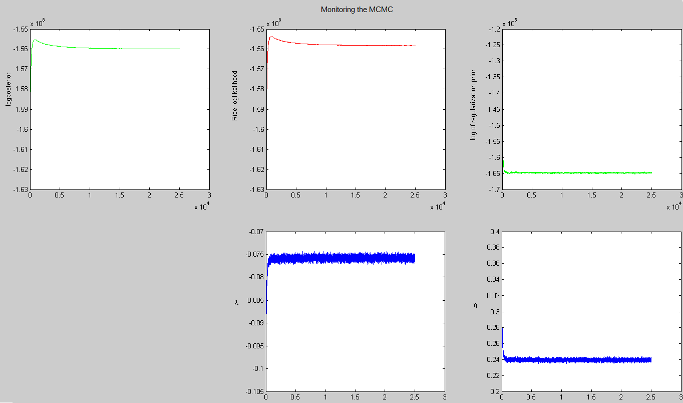
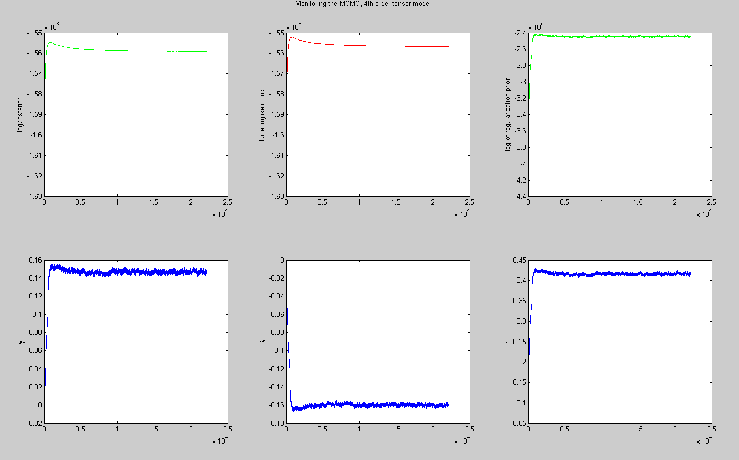
Before computing empirical averages, we waited for the Markov chain to reach stationarity. The burnin-period ($15600$ and $10450$ cycles under the 2nd and 4th-order tensor models, respectively) was selected by monitoring the logposterior and the regularization parameters of the samples shown in Fig. 1, which deserves an explanation. We see that the Rice-loglikelihood increases first very rapidly, and then decreases before stabililizing. Such phenomena is not uncommon in high dimensional models, when a maximum likelihood estimator is used to construct the initial configuration (see for example Fig. 3 in Besag J. et al. (1995)). To see this effect in a toy model, just consider a Gaussian vector $X\in\mathbb{R}^{n}$ with i.i.d. coordinates $X_{i}\sim{\mathcal{N}}(\theta,\sigma^{2})$, which satisfies

$$\sup_{x\in\mathbb{R}^{n}}\bigl{\{}\log p_{n}(x)\bigr{\}}-E_{P}\bigl{(}\log p_{n}(X)\bigr{)}=\frac{n}{2}\;.$$ (4.25)

In high dimension, under the posterior distribution the typical configuration and the maximum a posteriori (MAP) configuration can be very different, with a set of typical configurations containing most of the probability mass, while the probability mass concentrated around the MAP-configuration is negligible. Since we start the Markov chain from the maximum likelihood estimator under the approximating log-normal model, at the beginning the orientation of all tensors (but not their eigenvalues) are close to optimal also under the exact Rice likelihood model. Then the tensor eigenvalues and noise parameters move rapidily towards configurations with highest posterior probability. After this phase, it takes a while for the tensor orientations to mix-up. Since the acceptance probabilities are not uniform betwteen blocks, and we are estimating simultaneously the regularization parameters, the total logposterior density shows a slow decay before reaching stationarity.

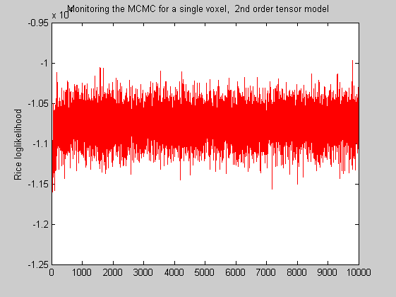
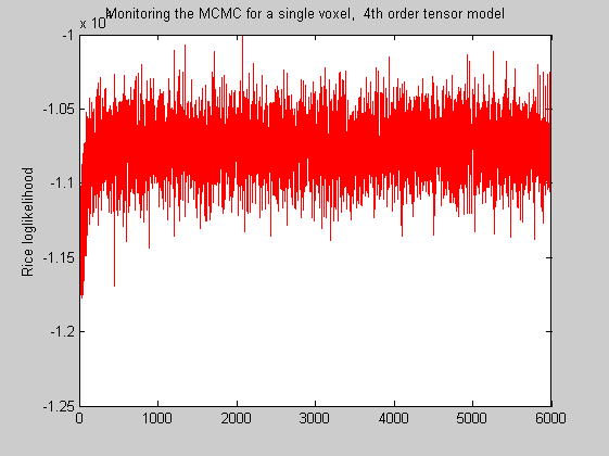
For comparison, we plot in Fig. 2 the McMC trace of the Rician loglikelihood for a single voxel under 2nd and 4th tensor models, without Bayesian regularization, which converges rapidly to stationarity.

(a) 2nd order tensor model, 25050 cycles

(b) 4th order tensor model, 22100 cycles

Figure 1: McMC traces of total posterior density, likelihood and prior (in logarithmic scale), and regularization parameters $\lambda,\eta$ and $\gamma$, for 2nd and 4th-order tensor models.

(a) 2nd order tensor model, 10000 cycles

(b) 4th order tensor model, 6000 cycles

Figure 2: McMC trace of the Rician loglikelihood for a single voxel, under the 2nd and 4th-order tensor models (without Bayesian regulatization)

Acceptance probabilities

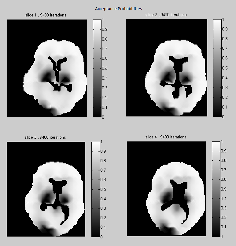
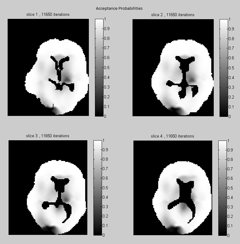
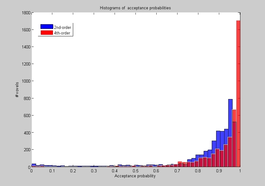
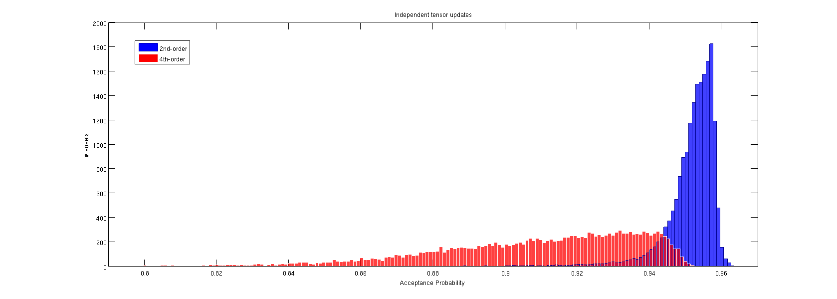
In Fig. 3 we show the acceptance probabilities for the Gibbs-Metropolis block update of the tensor parameters, estimated for each voxel under the regularized 2nd and 4th order tensor models. Note that, although we use large block updates with more than 300 voxels in each block, the acceptance probabilities are remarkably high in most of the voxels (see the histograms). It means that in most cases the our Gaussian approximation is very close to the exact full conditional distribution of the tensor parameters in a block. Note also that in Fig. 3(a) (which corresponds to 2nd order tensor model) there are some regions with lower acceptance probability. In such areas one should use update blocks of smaller size. These regions of lower acceptance probability are either artefacts, where the data are corrupted, or contain complex structures where the 2nd order tensor model does not fit well the data, and a higher order model would be more appropriate. We see two low acceptance probability regions situated symmetrically on the left and right sides of the ventricles. Anatomically this corresponds to the corona radiata where fiber bundles from multiple directions are crossing. By comparing with Fig. 3(b) we see that in these regions the acceptance probability improves under the (regularized) 4th order tensor model. For the diffusion model without regularization, the independent tensor updates have high acceptance probabilities at all voxels, under both 2nd and 4th-order tensor models (in 5).

(a) acceptance probability, 2nd order tensor model

(b) acceptance probability, 4th order tensor model

Figure 3: Acceptance probabilities in grey level scale (black=0,white=1) for the 2nd and 4th-order regularized tensor models

Figure 4: Acceptance probabilities across voxels for tensor block updates, under 2nd and 4th order regularized tensor models.

Figure 5: Acceptance probabilities across voxels for tensor independent updates, without regularization, under 2nd and 4th order models.

Deviance Information Criterion

The deviance information criterion (DIC), introduced by Spiegelhalter, D.J. et al. (2002), is a measure of model fitting used in Bayesian model selection as an alternative to Bayes factors. Unlike Bayes factors, DIC is well defined also when improper priors are assumed, as it is the case in our settings. It is defined as

$$\mbox{DIC}=2E_{\pi}\bigl{(}D(\theta)\big{|}\mbox{data}\bigr{)}-D\bigl{(}E_{\pi}(\theta|\mbox{data})\bigr{)},$$

where $D(\theta)=-2\log p(\mbox{data}|\theta)$ is the deviance, and we take conditional expectations with respect to the posterior distribution of the parameters $\theta$. Defined in analogy with the toy example of Eq. (4.25), the effective number of parameters

$$n_{eff}:=D\bigl{(}E_{\pi}(\theta|\mbox{data})\bigr{)}-E_{\pi}\bigl{(}D(\theta)\big{|}\mbox{data}\bigr{)}$$

appears as penalization term in the expression

$$\mbox{DIC}=-E_{\pi}\bigl{(}\log p(\mbox{data}|\theta)\big{|}\mbox{data}\bigr{)}+n_{eff}\;.$$

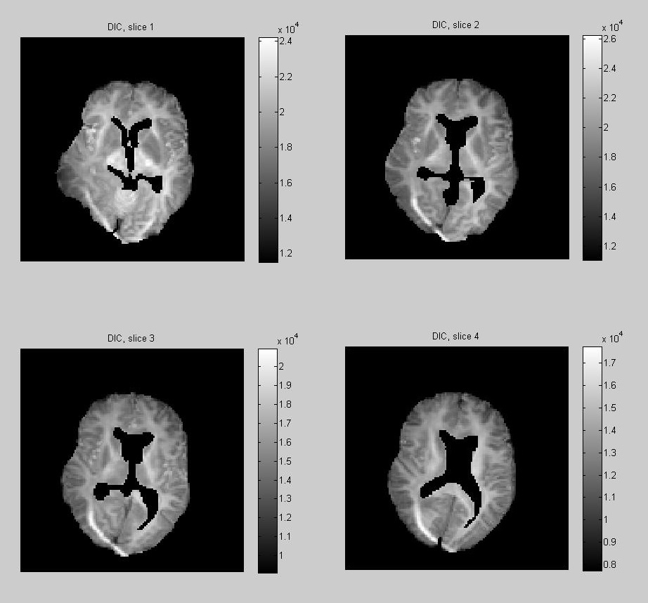
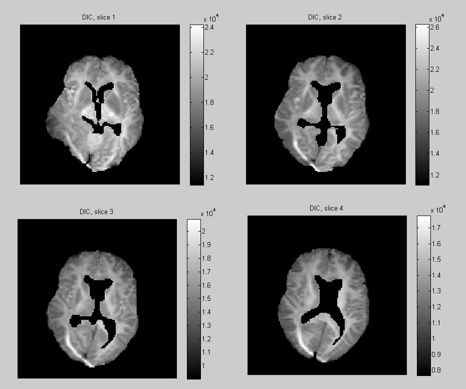
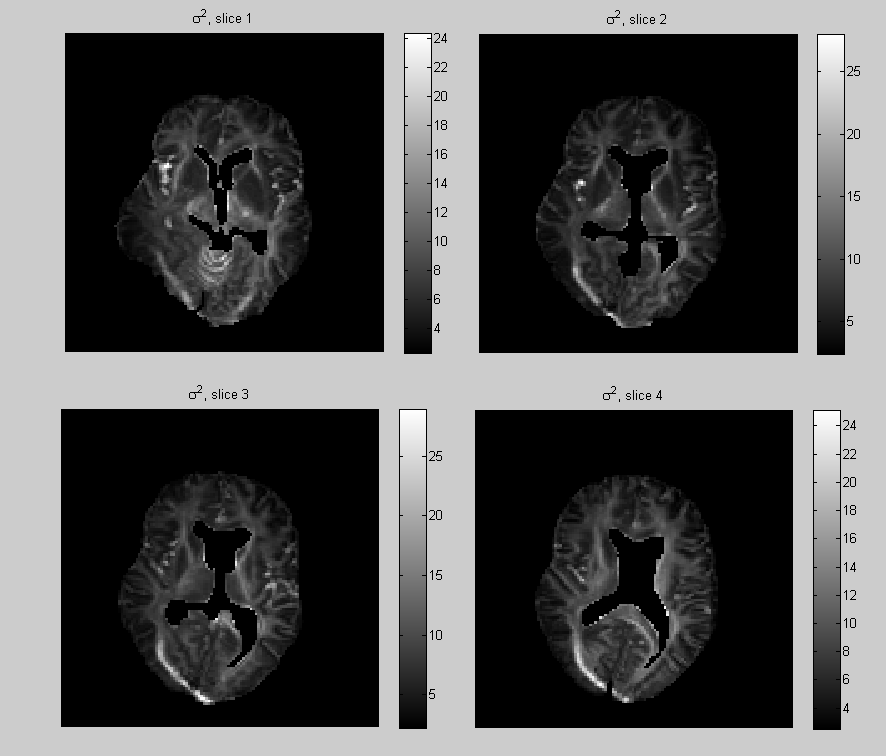
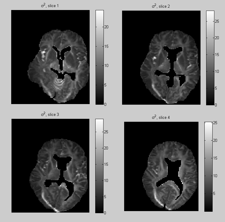
This allows for model comparisons, lower DIC meaning a better fit to the data relatively to the effective number of parameters. In Fig. 6 the DIC is computed independently at each voxel under the 2nd and 4th-order tensor models (without regularization). Note that the voxels with the highest DIC corresponds to artefacts where the data is corrupted, and the area of high DIC correspond to complex white matter structures. We also calculated the overall DIC for all voxel under the model 2nd and 4th-order tensor models with regularization. The respective values DIC$=-1.5554\times 10^{8}$ and DIC$=-1.5525\times 10^{8}$, indicate that when we penalize the model by the effective number of parameters, overall the 2th-order tensor model fits our data better than the 4th-order model. In Fig. 7 the posterior expectation of the noise parameters $\sigma^{2}(v)$, are shown. When these are interpreted as residual variances in model fitting, we see that they are consistent with the DIC.

(a) 2nd order independent tensor model

(b) 4th order independent tensor model

Figure 6: DIC maps under 2nd and 4th-order tensor model without regularization. Lower values (dark) correspond to better model fit.

(a) posterior expectation, 2nd order tensor model

(b) posterior expectation 4th order tensor model

Figure 7: Posterior expectations of the variance parameters in the Rician noise distribution, in 2nd and 4th-order tensor models

Diffusivity profiles

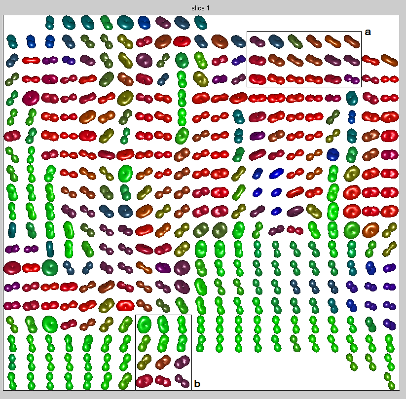
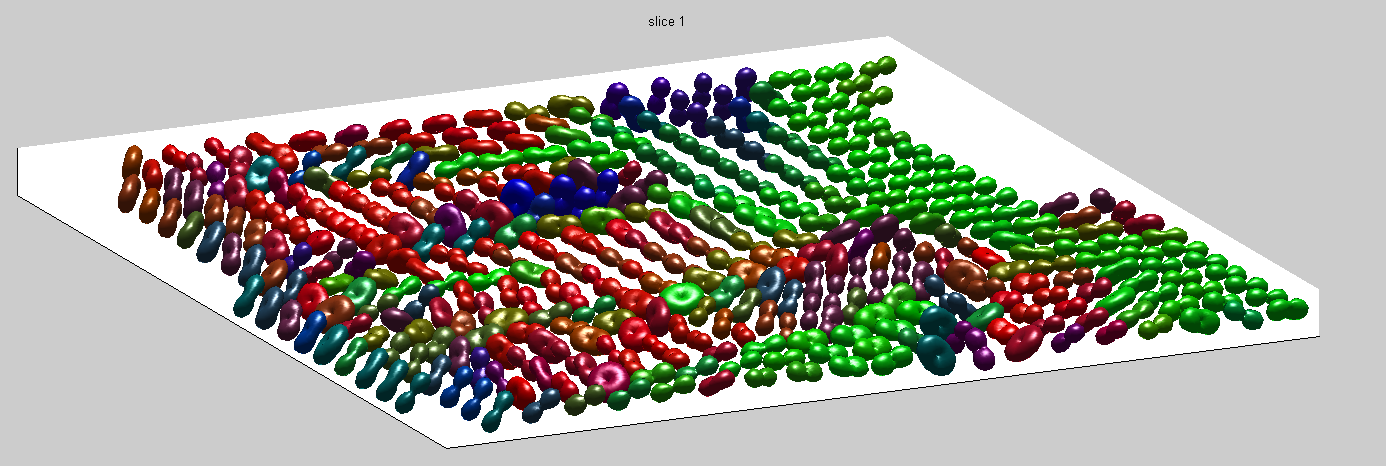
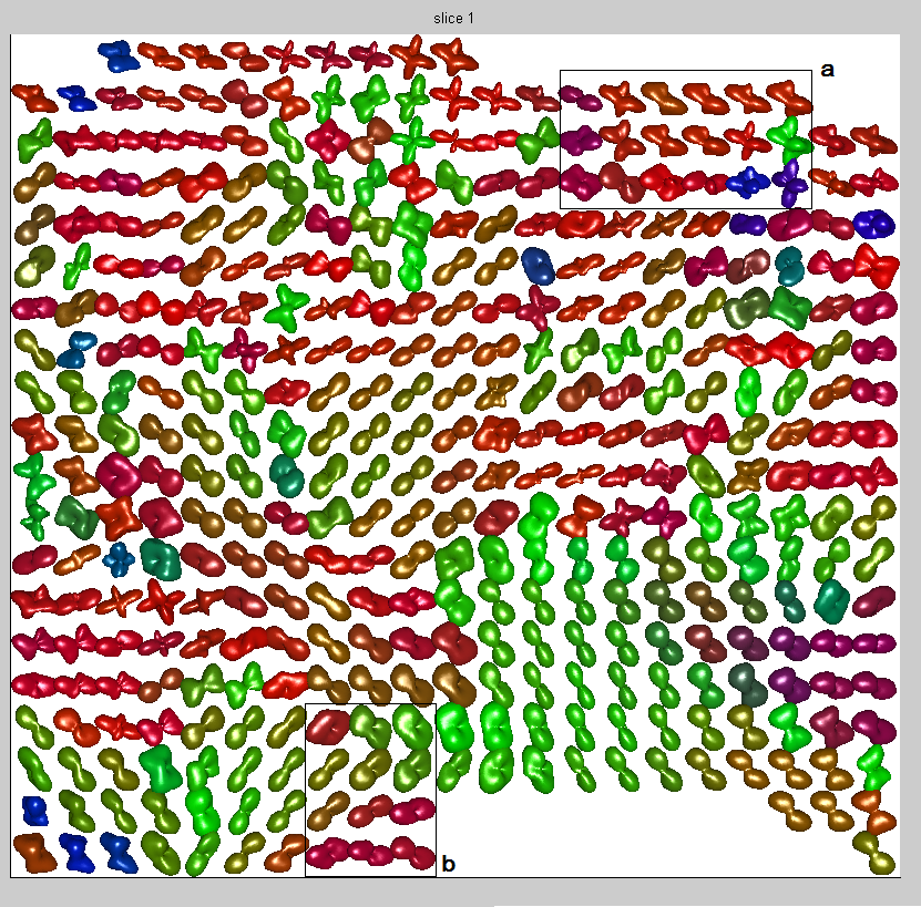
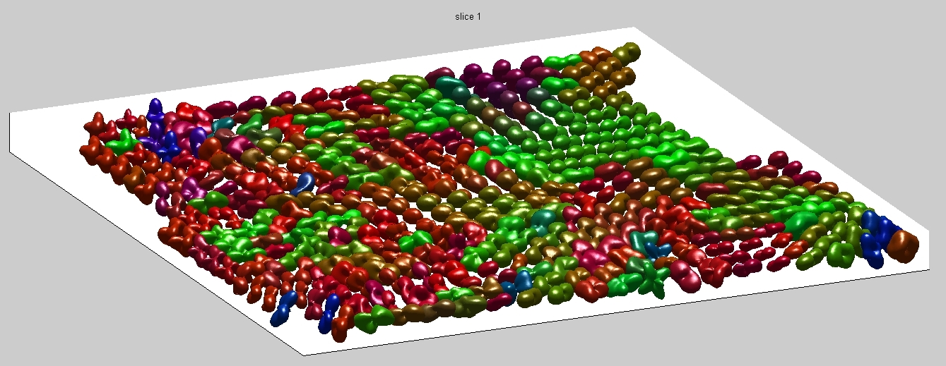
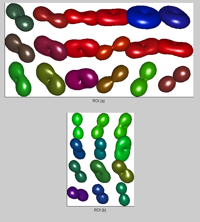
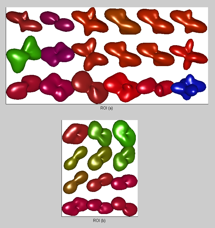
Fig. 8 shows the diffusivity profiles based on the posterior estimates of the tensors at all voxels in a region of interest. For each direction $u\in{\mathcal{S}^{2}}$ and spatial location $v\in V\subset\mathbb{R}^{3}$, we plot the point $(v+\overline{d_{v}(u)}u)\in\mathbb{R}^{3}$, where $\overline{d_{v}(u)}$ is the posterior expectation of the diffusivity. In order to observe the differences between 2nd and 4th order tensor models, in Fig. 9 we zoom into the ROI (a) and (b), and see that the 4th order tensor model captures the fiber-crossings which the 2nd order model cannot capture. At the fiber-crossing locations, under the 2nd-order model the two largest eigenvalues of the estimated tensor have similar sizes, with a donut-shaped diffusivity profile.

(a) Estimated diffusivity profiles under 2nd-order tensor model

(b) Estimated diffusivity profiles under 4th-order tensor model

Figure 8: Estimated diffusivity profiles from a ROI, under 2nd and 4th-order tensor model. The color-code represents the main direction of the principal eigenvalue of the 2nd-order tensor: Red, left-right; Green, anterior-posterior; Blue, superior-inferior. These figures are drawn with the Matlab package fanDTasia written by Barmpoutis (Barmpoutis A., Vemuri B.C., 2010; Barmpoutis A. et al., 2009).

(a) 2nd order

(b) 4th-order

Figure 9: Estimated diffusivity profiles under 2nd and 4th-order tensor models in ROI (a), showing crossing fibers between the corticospinal tract and superior longitudinal fibers, and ROI (b), showing fiber crossing near the corpus callosum, both selected from Fig. 8

Bayesian regularization

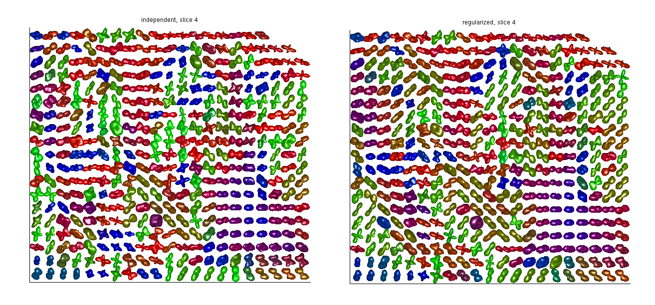
In Fig. 10 we compare diffusivity profiles from a region of interest without and with regularization, under the 4th order tensor model. With regularization, the differences in shape and direction between neighbouring tensors get smoothed. This also implies noise reduction: the tensor information from data corrupted by artefacts is corrected by the information from the neighbours. For the 2nd-order tensor model, the regularization effect in the same region was not that evident. Since the regularization parameters are not fixed but estimated from the data, we cannot always expect an increase from the smoothness level determined by the data. In order to achieve a prespecified level of smoothness we should either fix the regularization parameters or assign them a strongly informative prior. The posterior mean and standard deviation of the regularization parameters is given in Table 1.

	$\bar{\eta}$	$\sqrt{ \overline{\eta^{2}}-(\bar{\eta})^{²}}$	$\bar{\lambda}$	$\sqrt{ \overline{\lambda^{2}}-(\bar{\lambda})^{2}}$	$\bar{\gamma}$	$\sqrt{ \overline{\gamma^{2}}-(\bar{\gamma})^{2}}$
2nd order	0.2394	0.0012	-0.0758	$3.9352\times 10^{-4}$
4th order	0.4155	0.0021	-0.1600	0.0012	0.1469	0.0016

Table 1: Posterior mean and standard deviation of regularization parameters

Figure 10: Diffusivity profiles from a ROI under 4th-order tensor model, estimated with and without regularization.

Fractional Anisotropy and Mean Diffusivity.

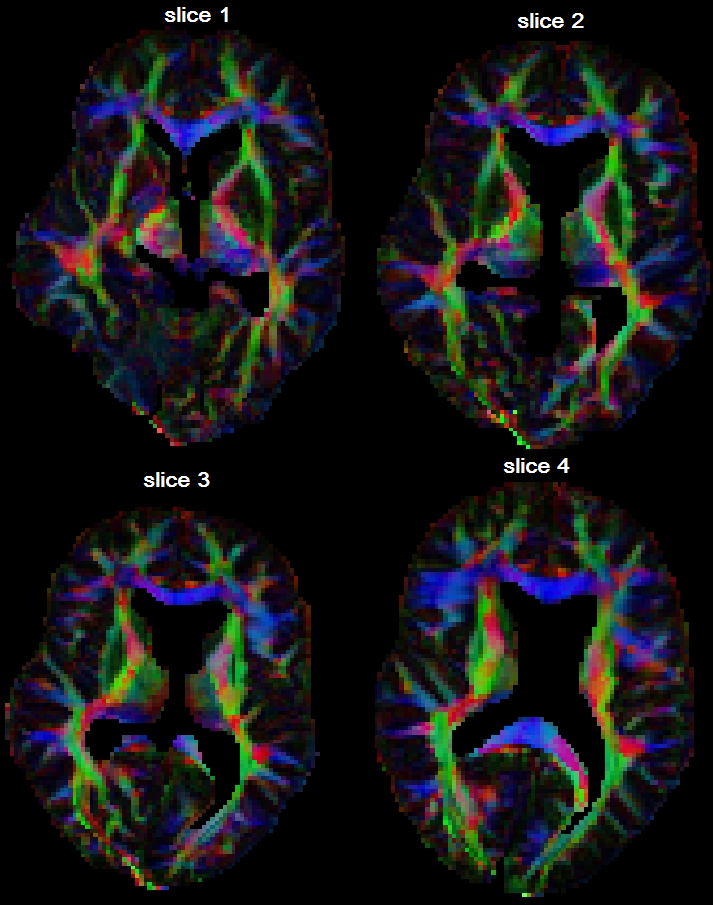
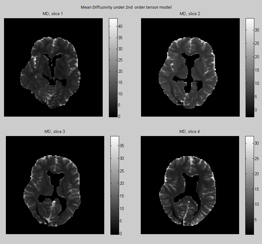
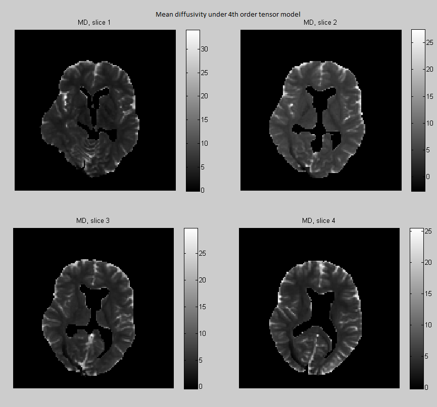
Fractional anisotropy (FA) measures the degree of anisotropy, while mean diffusivity (MD) is the average of the diffusivity $d(u)$ function over the unit sphere. Both measures are used as biomarkers to study brain pathologies. These quantities are expressed in terms of the eigenvalues of the 2nd order tensor as

$$\text{MD}=(\lambda_{1}+\lambda_{2}+\lambda_{3})/3,\quad\text{FA}={\frac{{\sqrt{3((\lambda_{1}-MD)^{2}+(\lambda_{2}-MD)^{2}+(\lambda_{3}-MD)^{2})}}}{{\sqrt{2(\lambda_{1}^{2}+\lambda_{2}^{2}+\lambda_{3}^{2})}}}},$$

In Section 3.9 we have seen that there is a linear bijection between the tensor coefficients and the coefficients of the truncated spherical harmonic expansion of the diffusivity. This implies that we can map linearly a 4th-order tensor to a 2nd-order tensor as follows (see Özarslan E., Mareci T.H. (2003)):

$$D_{11} =\frac{3}{35}(9D_{1111}+8D_{1122}+8D_{1133}-D_{2222}-D_{3333}-2D_{2233})$$

$$D_{22} =\frac{3}{35}(9D_{2222}+8D_{1122}+8D_{2233}-D_{1111}-D_{3333}-2D_{1133})$$

$$D_{33} =\frac{3}{35}(9D_{3333}+8D_{1133}+8D_{2233}-D_{1111}-D_{2222}-2D_{1122})$$

$$D_{12} =\frac{6}{7}(D_{1112}+D_{2223}+D_{1233})$$

$$D_{13} =\frac{6}{7}(D_{1113}+D_{1333}+D_{1223})$$

$$D_{23} =\frac{6}{7}(D_{2223}+D_{2333}+D_{1123}),$$

and the mean diffusivity can be also expressed in terms of the 4th order tensor coefficients as

$$\text{MD}=\frac{1}{5}(D_{1111}+D_{1122}+D_{1133}+2D_{2222}+2D_{3333}+2D_{2233}=\frac{1}{5}\text{trace}(\widehat{D}),$$ (4.26)

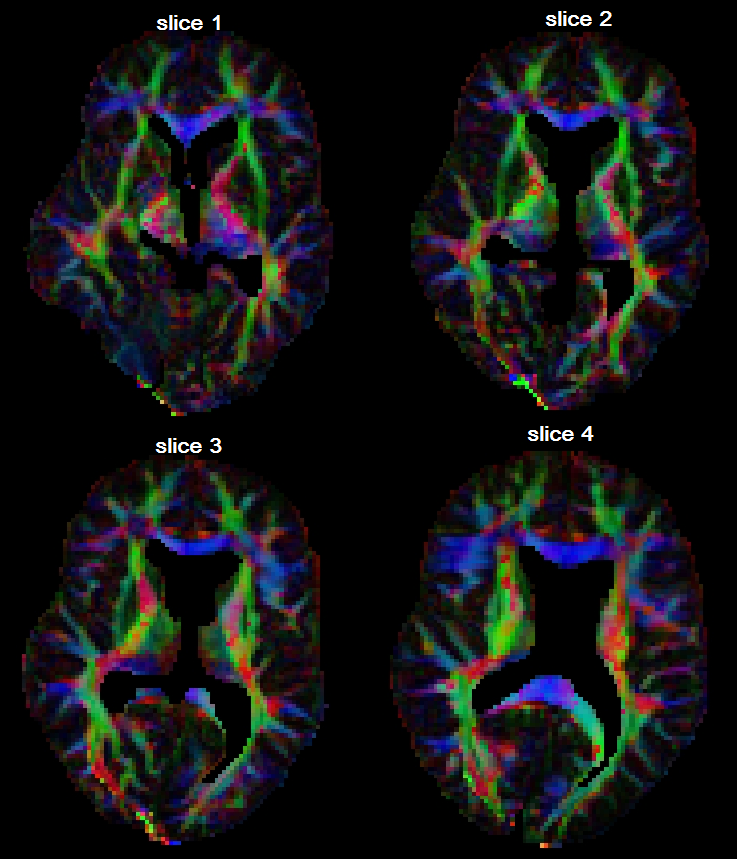
where $\widehat{D}$ was defined in Eq. (3.18). In Fig. 11 and 12 we compare the respectively the Bayesian estimates of FA and MD derived under the 2nd and 4th-order tensor models.

(a)

(b)

Figure 11: Bayesian FA estimates under 2nd (Fig. 11(a)) and 4th (Fig. 11(b)) order tensor models. As in the previous figures, the color-code shows the orientations of the principal eigenvalue of the 2nd order tensor, with intensities proportional to the fractional anisotropy.

(a)

(b)

Figure 12: The mean diffusivity (MD) maps from the results for both 2nd (Fig. 12(a)) and 4th (Fig. 12(b)) order diffusion tensor.

5 Conclusion

Rician noise, which models the magnitude of a real valued signal perturbed by additive complex Gaussian noise, appears in a wide range of applications in statistics and signal processing. By using a novel representation of the Rician likelihood, we are able to reduce nonlinear regression problems with Rician noise to Generalized Linear Models with Poissonian noise. This representation turns out to be very useful in Diffusion Tensor Imaging, where the problem is to estimate the transition distribution of water molecules diffusing inside the brain cells, by using spectral data which is corrupted by Rician noise. In this work we parametrize these transition distributions with diffusion tensors of either 2nd or 4th order.

We follow the Bayesian paradigm, choosing improper non-informative priors for tensors and noise parameters. Indeed, in the Bayesian regularization of the tensor field only very little assumptions are needed, namely an improper and isotropic Gaussian Markov random field prior, where the regularization parameters with scale invariant priors are also estimated from the data. This is very much in the spirit of E.T. Jaynes who advocated for Bayesian inference using objective priors, which should be based on symmetries and on the maximum entropy principle when prior information is not available (Jaynes E.T. (2002)). It is also not far from the penalized maximum likelihood approach, with the difference that we use as Bayesian estimator the posterior expectations rather than the Maximum A Posteriori configuration (which again could be obtained by simulated annealing after adding a temperature parameter to our Gibbs-Metropolis algorithm).

Although Bayesian regularization has already been used in the diffusion-MRI literature, until now McMC was not seen as a viable alternative for the analysis of high $b$-value diffusion-MR data. To obtain diffusion images, we need to process an huge amount of data. Standard McMC strategies like single site updates and random walk proposals were not efficient enough to produce whole brain images under the Rice noise model. By exploiting the properties of Generalized Linear Models, we are able to construct a Gaussian approximation to the full conditional distribution and update simultaneously large blocks of tensor variables with high acceptance rates. It is clear that our fully Bayesian approach, as well as all methods based on penalized maximum likelihood, is computationally extensive compared with multi-stage procedures where first the tensors are estimated independently, and only in a second step smoothing and interpolation procedures are applied. However second-stage smoothing has its drawbacks, for example it depends on the choice of the tensor metrics, it can induce unwanted effects as tensor swelling (Dryden I.L. et al., 2009). Nowadays there are affordable options for acceleration, e.g. adopting parallel computation on a large computer cluster, and computing with Graphical Processor Unit (GPU) (Hernández M. et al., 2013). On the other hand, the acquisition of MR-diffusion data is very costly and we cannot keep a subject for hours inside the scanner, in order to get the most out of the data it makes sense to use more computational resources and perform an accurate Bayesian computation under the exact noise model combining estimation and adaptive regularization in single procedure.

We are currently working to extend our framework in several directions. In a forthcoming paper, we have implemented the variational Bayes (VB) approximation of the posterior distribution under the very same Bayesian hierarchical model discussed in this work. We are also working on positive definite tensor models, as the ternary quartic approach (Barmpoutis A., Vemuri B.C., 2010),(Ghosh A, 2011),(Ghosh A. et al., 2009), and on spherical harmonic expansions with variable dimensions, with random truncation levels at each voxel, and using reversible-jump McMC to sample from the posterior (Green P.J., 1995). This would produce a brain segmentation with classification of the voxels according to the tensors order.

Appendix

Appendix A Sampling from the reinforced Poisson distribution

1. The standard way by using the cumulative distribution function:

   $$X(\omega)=\min\biggl{\{}n:\;\sum\limits_{k=0}^{n}\frac{\tau^{2k}}{(k!)^{2}}\;\geq\;{}_{0}F_{1}(1,\tau^{2})\;\omega\biggr{\}}.$$

   with $\omega$ uniformly distributed in $[0,1]$. This requires evaluation of the normalizing constant ${}_{0}F_{1}(1,\tau^{2})$.

2. A direct but unefficient rejection method:

   Generate $N\sim\mbox{Poisson}(\tau)$, accept it and set $X=N$ with probability $P_{\tau}(N^{\prime}=N|N)=\exp(-\tau)\tau^{N}/N!$ where $N^{\prime}$ is an independent copy of $N$, otherwise repeat until acceptance.

3. An improved rejection sampler, the one actually used. Generate independenty $N\sim\mbox{Poisson}(\alpha)$ and $\omega$ uniform in $[0,1]$,
   until

   $$\frac{\tau^{2N}}{(N!)^{2}}\frac{1}{\pi_{\alpha}(N)}=\frac{(\tau^{2}/\alpha)^{N}}{N!}\exp(\alpha)\geq C(\alpha,\tau)\;\omega$$

   where

   $$C(\alpha,\tau):=\max_{n}\biggl{\{}\exp(\alpha)\frac{(\tau^{2}/\alpha)^{n}}{n!}\biggr{\}}=\frac{(\tau^{2}/\alpha)^{n^{*}}}{n^{*}!}\exp(\alpha)$$ (A.1)

   and $n^{*}=\lfloor\tau^{2}/\alpha\rfloor$ is the mode of a Poisson distribution with parameter $\tau^{2}/\alpha$, ( $\lfloor\cdot\rfloor$ denotes the floor function). Return $X=N$.

   For large $\tau$, assuming apriori that at optimality $\alpha\ll\tau^{2}$, by using Stirling’s approximation $\log(n!)\approx(n\log(n)-n)$, we find that the proposal parameter $\alpha(\tau)=\tau$ is approximately optimal.

References

- Andersson J.L.R. (2008) Andersson J.L.R. 2008. Maximum a posteriori estimation of diffusion tensor parameters using a Rician noise model: Why how and but. Neuroimage 42(4) 1340-1356.
- Assemlal, H.E. et al. (2009) Assemlal, H.E., Tschumperlé D., Brun L. 2009. Efficient and robust computation of PDF features from diffusion MR signal. Medical Image Analysis 13:5 715-729.
- Barmpoutis A. et al. (2009) Barmpoutis, A. and Hwang, M.S. and Howland, D. and Forder, J.R. and Vemuri, B.C., 2009. Regularized positive-definite fourth order tensor field estimation from DW-MRI. NeuroImage, S153-S162.
- Barmpoutis A., Vemuri B.C. (2009) Barmpoutis A., Vemuri B.C., 2009. Groupwise Registration and Atlas Construction of 4th-Order Tensor Fields Using the Riemannian Metric. Medical Image Computing and Computer-Assisted Intervention – MICCAI 2009, Springer Lecture Notes in Computer Science 5761, 640-647.
- Barmpoutis A., Vemuri B.C. (2010) Barmpoutis A., Vemuri B.C., 2010. A unified framework for estimating diffusion tensors of any order with symmetric positive-definite constraints. Biomedical Imaging: From Nano to Macro 2010 IEEE Int. Symp, 1385-1388.
- Basser PJ, Mattiello J, Le Bihan D. (1994) Basser P.J., Mattiello J., Le Bihan D., 1994. Estimation of the effective self-diffusion tensor from the NMR spin echo. J. Magn. Reson. B 103(3), 247-254.
- Basser P.J., Pajevic S. (2007) Basser P.J., Pajevic S., 2007. Spectral decomposition of a 4th-order covariance tensor: Applications to diffusion tensor MRI. Signal Processing 87, 220-236
- Basser P.J., Pajevic S. (2003) Basser P.J., Pajevic S., 2003. A normal distribution for tensor-valued random variables: applications to diffusion tensor MRI. IEEE Trans. Med. Imag. 22 (7), 785-794.
- Behrens. T.E.J. et al. (2003) Behrens T.E.J. ,Woolrich M.W. ,Jenkinson M. , Johansen-Berg H., Nunes R.G., Clare S. ,Matthews P.M. , Brady J.M., Smith S.M. 2003. Characterization and Propagation of Uncertainty in Diffusion-Weighted MR Imaging. Magnetic Resonance in Medicine 50:1077–1088.
- Besag J. et al. (1991) Besag, J., York, J., Mollié A. (1991). Bayesian image restoration, with two applications in spatial statistics. Ann. Inst. Statist. Math. 43 (1) 1–59.
- Besag J. et al. (1995) Besag J., Green P., Higdon D., Mengersen K. 1995. Bayesian computation and stochastic systems (1995). Statistical Science 10:1, 3–66.
- Burdette, J.H. et al. (2001) Burdette, J.H., Durden, D.D., Elster, A.D., Yen, Y.F., 2001. High b-value diffusion-weighted MRI of normal brain. J. Comput. Assi. Tomogr. 25(4), 515.
- Carr H.Y., Purcell E.M. (1954) Carr H.Y., Purcell E.M., 1954. Effects of diffusion on free precession in nuclear magnetic resonance experiments. Phys. Rev. 94(3), 630-638.
- Dryden I.L. et al. (2009) Dryden I.L.,Koloydenko A., Zhou D. 2009. Non-Euclidean statistics for covariance matrices, with applications to diffusion tensor imaging Annals of Applied Statistics 3 (3) 881-1231.
- Frandsen, J. et al. (2007) Frandsen, J., Hobolth, A., Østergaard, L., Vestergaard-Poulsen, P., Jensen, E.B.V., 2007. Bayesian regularization of diffusion tensor images. Biostatistics 8 (4), 784-799.
- Geman S. and Geman D. (1984) Geman S., Geman D., 1984. Stochastic Relaxation, Gibbs Distributions, and the Bayesian Restoration of Images. IEEE Trans. Pattern Anal. Mach. Intell. 6, 721-741.
- Ghosh A. et al. (2009) Ghosh A., Deriche R., Moakher M., 2009. Ternary quartic approach for positive 4th order diffusion tensors revisited. Biomedical Imaging: From Nano to Macro, ISBI’09. IEEE Int. Sym., pp. 618-621.
- Ghosh A (2011) Ghosh A., 2011. High Order Models in Diffusion MRI and Applications. PhD Thesis, Inria Sophia Antipolis.
- Ghosh A. et al. (2012) Ghosh A., Papadopoulo T. and Deriche R., 2012. Generalized Invariants of a 4th order tensor: Building blocks for new biomarkers in dMRI. Computational Diffusion MRI Workshop (CDMRI), MICCAI 165-173.
- Gradshteyn, I.S., Ryzhik, I.M. (2007) Gradshteyn, I.S., Ryzhik, I.M., 2007. Table of Integrals, Series, and Products, seventh edition. edited by Jeffrey, A., Zwillinger, D. Academic Press, pp. 918-920.
- Green P.J. (1995) Green P.J. 1995. Reversible Jump Markov Chain Monte Carlo Computation and Bayesian Model Determination. Biometrika, Vol. 82, No. 4. 711-732.
- Gudbjartsson H., Patz S. (2005) Gudbjartsson H., Patz S., 2005. The Rician distribution of noisy MRI data. Magn. Reson. Med., 34(6), 910-914.
- Hahn E. (1950) Hahn E., 1950. Spin echoes. Phys. Rev. 80, 580–594.
- Hagmann P. et al. (2006) Hagmann, P., Jonasson, L., Maeder, P., Thiran, J.P., Wedeen, V.J., Meuli, R., 2006. Understanding Diffusion MR Imaging Techniques: From Scalar Diffusion-weighted Imaging to Diffusion Tensor Imaging and Beyond, Radiographics, 26(suppl 1), S205-S223.
- Hastings W.K. (1970) Hastings W.K., 1970. Monte Carlo sampling methods using Markov chains and their applications. Biometrika 57 (1), 97-109.
- Henkelman R.M. (1985) Henkelman R.M., 1985. Measurement of signal intensities in the presence of noise in MR images. Med. phys., 12(2), 232-233.
- Hernández M. et al. (2013) Hernández M., Guerrero G.D., Cecilia J.M., Garcia J.M., Inuggi A., Jbabdi S., Behrens T.E.J. 2013. Accelerating Fibre Orientation Estimation from Diffusion Weighted Magnetic Resonance Imaging Using GPUs. PlosOne 0061892.
- Huisman, T.A.G.M. et al. (2006) Huisman, T.A.G.M., Loenneker, T., Barta, G., Bellemann, M.E., Hennig, J., Fischer, J.E., Il’yasov, K.A., 2006. Quantitative diffusion tensor MR imaging of the brain: field strength related variance of apparent diffusion coefficient (ADC) a nd fractional anisotropy (FA) scalars. Eur. radiol. 16(8), 1651-1658.
- Jaynes E.T. (2002) Jaynes E.T., 2002. Probability, the Logic of Science. Cambridge University Press.
- Jeffreys H. (1961) Jeffreys H., 1961. Cartesian Tensors. Cambridge University Press.
- Jian B., Vemuri B.C. (2007) Jian B., Vemuri B.C., 2007. Multi-fiber Reconstruction from Diffusion MRI Using Mixture of Wisharts and Sparse Deconvolution. IPMI, pp. 384-395.
- Jones D.K., Basser P.J. (2004) Jones D.K., Basser P.J., 2004. "Squashing peanuts and smashing pumpkins": How noise distorts diffusion-weighted MR data. Magn. Reson. Med. 52(5), 979-993.
- Krissian K. Aja-Fernandez S. (2009) Krissian, K., Aja-Fernández S. (2009). Noise-driven anisotropic diffusion filtering of MRI. IEEE Transactions on Image Processing 18 (10) 2265-2274.
- Kaipio J., Somersalo E. (2005) Kaipio J., Somersalo E., 2005. Statistical and Computational Inverse Problems. Springer.
- Koay et al. (2006) Koay C.G., Chang L.C., Carew J.D., Pierpaoli C., Basser P.J., 2006. A unifying theoretical and algorithmic framework for least squares methods of estimation in diffusion tensor imaging. Journal of Magnetic Resonance 182(1): 115-125.
- Koay C.G., Özarslan E., Basser P.J. (2009) Koay C.G., Özarslan E., Basser P.J., 2009. A signal transformational framework for breaking the noise floor and its applications in MRI, J. Magn. Reson., 197(2), 108-119.
- Landman B. et al (2007) Landman B. Bazin P-L. and Prince J. 2007. Diffusion tensor estimation by maximizing Rician likelihood. 11th IEEE International Conference on Computer Vision ICCV 2007.
- Lange K. (2013) Lange K (2013). Optimization (2nd Edition). Springer Texts in Statistics Vol. 95. Springer New York.
- Lauterbur P.C. (1973) Lauterbur P.C., 1973. Image formation by induced local interactions: examples employing nuclear magnetic resonance. Nature 242 (5394), 190-191.
- Lauwers L. et al. (2010) Lauwers L., Barbé K., Van Moer W., Pintelon R., 2010. Analyzing Rice distributed functional magnetic resonance imaging data: a Bayesian approach. Measurement Science & Technology 21, 115804.
- Le Bihan D et al. (1986) Le Bihan D., Breton E., Lallemand D., Grenier P., Cabanis E., Laval-Jeantet M., 1986. MR imaging of intravoxel incoherent motions: application to diffusion and perfusion in neurologic disorders. Radiology 161(2), 401-407.
- Leemans A et al. (2009) Leemans, A., Jeurissen, B., Sijbers, J., Jones, D.K., 2009. ExploreDTI: a graphical toolbox for processing, analyzing, and visualizing diffusion MR data. Proc. Intl Soc. Mag. Reson. Med 3537 Hawaii, USA.
- Liao Y. et al. (2010) Liao, Y., Tang, J., Ma, M., Wu, Z., Yang, M., Wang, X., Liu, T., Chen, X., Fletcher, P.C., Hao, W., 2010. Frontal white matter abnormalities following chronic ketamine use: a diffusion tensor imaging study. Brain, 133(7), 2115-2122.
- Marinucci D., Peccati G. (2011) Marinucci D, Peccati G. 2011. Random fields on the sphere. Representation, limit theorems and cosmological applications. London Mathematical Society Lecture Note Series, 389. Cambridge University Press, Cambridge,
- McCullagh, P., Nelder, J.A. (1989) McCullagh, P., Nelder, J.A., 1989. Generalized linear models 2nd Edition. Chapman & Hall/CRC.
- Metropolis N. et al. (1953) Metropolis N., Rosenbluth A.W., Rosenbluth M.N., Teller A.H. and Teller E., 1953. Equation of State Calculations by Fast Computing Machines. J.Chem. Phys. 21 (6), 1087-1092.
- Moakher M. (2009) Moakher M., 2009. The algebra of fourth-order tensors with application to diffusion MRI. In: Laidlaw D.H., Weickert J. (Eds.) Vis. Process. Tensor Fields Advan. Perspect., Springer, pp. 57.
- Mori S., Tournier J.D. (2014) Mori S., Tournier J.D., 2014. Introduction to Diffusion Tensor Imaging and Higher Order Models, 2nd Edition. Elsevier Science.
- Moseley ME et al. (1990) Moseley M.E., Cohen Y., Kucharczyk J., Mintorovitch J., Asgari H.S., Wendland M.F., Tsuruda J., Norman D., 1990. Diffusion-weighted MR imaging of anisotropic water diffusion in cat central nervous system. Radiology 176(2), 439-445.
- Nummelin E. (2002) Nummelin E., 2002. MC for MCMC’ists. Int. Stat. Rev. 70 (2), 215-240.
- Özarslan E., Mareci T.H. (2003) Özarslan E., Mareci T.H., 2003. Generalized diffusion tensor imaging and analytical relationships between diffusion tensor imaging and high angular resolution diffusion imaging. Magn. Reson. Med. 50 (5), 955-965.
- Özarslan E. et al. (2005) Özarslan E., Vemuri C. B., and Mareci T.H., 2005. Generalized scalar measures for diffusion MRI using trace, variance, and entropy. Magn. Reson. Med. 53 (4), 866–876.
- Pajevic S., Basser P.J. (2003) Pajevic S., Basser P.J., 2003. Parametric and non-parametric statistical analysis of DT-MRI data. J. Magn. Reson. 161 (1), 1-14.
- Qi L. et al. (2010) Qi L. Yu G., Wu E.X., 2010. Higher order positive semidefinite diffusion tensor imaging. SIAM J.Imag. Sci., 3(3), 416-433.
- Robert, C.P., Casella G. (2004) Robert, C.P., Casella G. 2004. Monte Carlo Statistical Methods, 2nd Edition, Springer Text in Statistics.
- Rue, H., Held, L. (2005) Rue, H., Held, L., 2005. Gaussian Markov Random Fields: Theory and Applications. Chapman & Hall/CRC, Boca Raton, FL.
- Salvador, R. et al. (2004) Salvador, R., Pena, A., Menon, D.K., Carpenter, T.A., Pickard, J.D., Bullmore, E.T., 2004. Formal characterization and extension of the linearized diffusion tensor model. Hum. brain mapp., 24(3), 144-155.
- Spiegelhalter, D.J. et al. (2002) Spiegelhalter, D.J., Best, N.G., Carlin, B.P. van der Linde, A., 2002. Bayesian measures of model complexity and fit. Journal of the Royal Statistical Society, B 64 (4): 583–639.
- Stejskal E.O., Tanner J.E. (1965) Stejskal E.O., Tanner J.E., 1965. Spin diffusion measurements: spin echoes in the presence of time-dependent field gradient. J. Chem. Phys., 42(1), 288-292.
- Torrey H. (1956) Torrey H., 1956. Bloch equations with diffusion terms. Phys. Rev. 104,563–565.
- Veraart, J. et al. (2011) Veraart, J., Van Hecke, W., Sijbers, J., 2011. Constrained maximum likelihood estimation of the diffusion kurtosis tensor using a Rician noise model. Magn. Reson. Med., 66(3), 678-686.
- Zhu H. et al. (2007) Zhu H., Zhang H., Ibrahim J.G., Peterson B.S., 2007. Statistical analysis of diffusion tensors in diffusion-weighted Magnetic resonance imaging Data. JASA 102 (480), 1085-1102.