Molecular line mapping of the giant molecular cloud associated with RCW 106 - IV. Ammonia towards dust emission

Abstract

Here we report observations of the two lowest inversion transitions of ammonia (NH3) with the 70-m Tidbinbilla radio telescope. The aim of the observations is to determine the kinetic temperatures in the dense clumps of the G333 giant molecular cloud associated with RCW 106 (hereafter known as the G333 GMC) and to examine the effect that accurate measures of temperature have on the calculation of derived quantities such as mass. This project is part of a larger investigation to understand the timescales and evolutionary sequence associated with high-mass star formation, particularly its earliest stages. Assuming that the initial chemical composition of a giant molecular cloud is uniform, any abundance variations within will be due to evolutionary state.

We have identified 63 clumps using SIMBA 1.2-mm dust continuum maps and have calculated gas temperatures for most (78 per cent) of these dense clumps. After using Spitzer GLIMPSE 8.0 ${\rm\mu m}$ emission to separate the sample into IR-bright and IR-faint clumps, we use statistical tests to examine whether our classification shows different populations in terms of mass and temperature. We find that in terms of log clump mass (2.44 – 4.12 M_⊙) and log column density (15.3 – 16.6 cm^-2), that there is no significant population difference between IR-bright and IR-faint clumps, and that kinetic temperature is the best parameter to distinguish between the gravitationally bound state of each clump. The kinetic temperature was the only parameter found to have a significantly low probability of being drawn from the same population. This suggests that clump radii does not have a large effect on the temperature of a clump, so clumps of similar radii may have different internal heating mechanisms. We also find that while the IR-bright clumps have a higher median log virial mass than the IR-faint clumps (IR-bright: 2.88 M_⊙; IR-faint: 2.73 M_⊙), both samples have a similar range for both virial mass and FWHM (IR-bright: log virial mass = 2.03 – 3.68 M_⊙, FWHM = 1.17 – 4.50 km s^-1; IR-faint: log virial mass = 2.09 – 3.35 M_⊙, FWHM = 1.05 – 4.41 km s^-1). There are 87 per cent (40 of 46) of the clumps with masses larger than the virial mass, suggesting that they will form stars or are already undergoing star formation.

1 INTRODUCTION

Figure 1: The G333 giant molecular cloud as seen in the infrared. The shocked gas (Spitzer 4.5 ${\rm\mu m}$), PAH⁺ emission (Spitzer 8.0 ${\rm\mu m}$) and cool dust (Herschel 160 ${\rm\mu m}$) are shown in blue, green and red, respectively. The contours are from the SIMBA 1.2 mm dust continuum emission at 0.1, 0.2, 0.5, 1, 1.5, 2.5, 5, 10 and 12 Jy/beam (as per the contours of fig. 4 of Mookerjea et al. 2004). The position of the peak emission within SIMBA dust clumps identified with clumpfind are overlaid with pink plus signs. The positions associated with RCW 106 have been overlaid with white stars (Rodgers et al., 1960).

The life cycles of high-mass ($\geq$8 M_⊙) stars have a major impact on the evolution of galaxies, while in turn, the position of a molecular cloud in the Galaxy has a major impact on the efficiency and type of star formation which occurs therein (Luna et al., 2006). However, exactly how these stars form, on what timescales and how they shape their environments during this active and energetic phase is poorly understood (see the review by Zinnecker & Yorke 2007).

The G333 giant molecular cloud (GMC), centred at $l$ = 333.^∘2, $b$ = -0.^∘4, is a 1.2° $\times$ 0.6° region of the southern Galactic Plane located at a distance of 3.6 kpc (Lockman, 1979) and is the fourth most active star forming region in the Galaxy (Urquhart et al., 2014). The complex forms part of the Galactic Ring of molecular clouds at a Galactocentric radius of 3-5 kpc, it contains the bright Hii regions RCW 106 (G332.9-0.6; Rodgers, Campbell & Whiteoak 1960) and G333.6-0.2 (Manchester, 1969), as well as high-mass star forming clumps, MSX infrared sources and Spitzer “Extended Green Objects” (Cyganowski et al., 2008). This cloud also contains the very young, high-mass star forming core G333.125$-$0.567 (Becklin et al., 1973; Garay et al., 2004; Lo et al., 2007; Lo et al., 2011) which is an isolated core at an evolutionary stage without any radio continuum or near-infrared detection. We have used the Mopra radio telescope to study the G333 GMC extensively in 20 molecular tracers including ¹³CO (Bains et al., 2006), C¹⁸O (Wong et al., 2008), HCN, HCO⁺, and N₂H⁺ (Lo et al., 2009).

In order to investigate a large sample of star forming clumps at different stages of evolution, we are conducting a multi-wavelength study of the G333 GMC. This region is within the area of the Spitzer GLIMPSE (3.6, 4.5, 5.8, 8.0 ${\rm\mu m}$; Benjamin et al. 2003; Churchwell et al. 2009) and MIPSGAL (24, 70 ${\rm\mu m}$; Carey et al. 2009), and the Herschel Hi-GAL (70, 160, 250, 350, 500 ${\rm\mu m}$; Molinari et al. 2010) surveys. Mookerjea et al. (2004) have defined multiple millimetre continuum clumps within this one molecular cloud, some associated with maser emission (e.g. Breen et al. 2007), as well as obvious polycyclic aromatic hydrocarbon (PAH) emission. We expect to have a range of evolutionary states within our clumps.

The ammonia (NH3) molecule can be used to probe the physical conditions within dense molecular gas. It has a large number of transitions that are sensitive to a variety of excitation conditions and can be detectable in both warm molecular gas and quiescent dark clouds. The rotational temperature and optical depth for each clump can be calculated from multiple (J,K) inversion transitions and their hyperfine components, respectively (Walmsley & Ungerechts, 1983). Hence the kinetic temperature can be calculated (Tafalla et al., 2004); however the lower (1,1) and (2,2) transitions are only useful for constraining temperatures lower than 30 K (Danby et al., 1988; Hill et al., 2010).

In this paper we report on the selection of dense clumps based on SIMBA dust emission and pointed NH3 (1,1) and (2,2) observations towards these clumps. Although finding the kinetic temperature is our main concern there are also several other physical parameters that can be determined from our measurements, including virial mass and column density. This is so we will have a sample of clumps within the G333 GMC, with clear selection criteria which will be used to compare the 3-mm molecular transitions and infrared Herschel and Spitzer dust surveys. We have chosen to study a single molecular cloud as the initial chemical composition of each clump should be very similar. Obtaining a reliable temperature measurement of each clump will allow us, in future papers, to calculate accurate molecular abundances for comparison between clumps.

2 OBSERVATIONS AND DATA REDUCTION

2.1 Selection of clumps

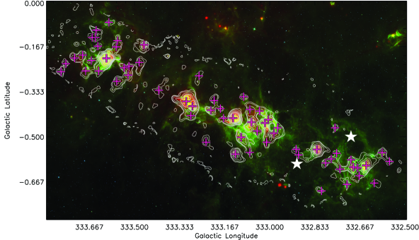
We have utilised the 1.2-mm dust continuum emission from the SIMBA instrument on the Swedish-ESO Telescope (SEST; Mookerjea et al. 2004) as a tracer for dense molecular material. To complement the density tracers from Bains et al. (2006), Wong et al. (2008) and Lo et al. (2009), we have convolved the Mookerjea et al. (2004) beam size from 24 arcsec to 36 arcsec, to match the beam size of the Mopra radio telescope at 100 GHz (Ladd et al., 2005). Using the starlink tool cupid, we have chosen the 2D clumpfind algorithm to automatically, but robustly, detect physically realistic clumps. The clumpfind algorithm works by identifying local maxima and includes all contiguous pixels down to the user-set contour level. If the contiguous pixels have already been identified in an earlier clump, then those pixels are included in that clump. For contiguous contours a “friends-of-friends” algorithm is used to assign the common pixels to a clump. These steps are repeated until the lowest level is reached. For a complete description of the clumpfind algorithm, see Williams, de Geus, & Blitz (1994). Using a 3$\sigma$ detection limit we have identified 63 clumps. The catalogue of clumps found in this paper differ from those in Mookerjea et al. (2004) because of the differing resolutions (24 arcsec versus 36 arcsec). The global positions are shown in Fig. 1, the local environment in Fig A, and the clumpfind results can be found in §3.1 and Table 1.

2.2 Ammonia from the 70-m Tidbinbilla radio telescope

Observations using the 70-m Tidbinbilla radio telescope were conducted in good weather conditions on 2011 July 11 and 12. Pointing errors were measured and corrected every few hours, by observing the quasar 1613-586, within 9^∘ from the target sources, yielding residual pointing errors smaller than 2 arcsec. System noise temperatures were in the range of $\sim$45-90 K, but typically $\sim$50 K. Sensitivity was $\sim$40-100 mK, but typically $\sim$50 mK. During these observations a left hand circularly polarized signal was recorded across two 64 MHz bands centred at 23708 and 23870 MHz, covering the NH3 (1,1) and (2,2) transitions in the first band and the (3,3) transition in the second band. With a bandwidth of 2048 channels across 64 MHz, each channel width was 31.25 kHz (or a velocity channel width of 0.4 km s^-1). Each source was observed for 2 min on-source integration.

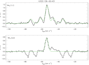
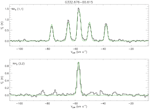
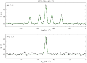
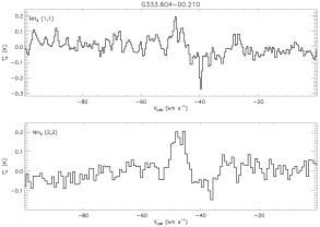
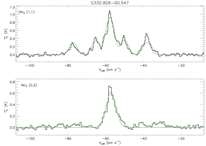
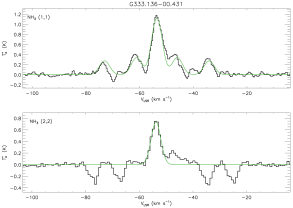
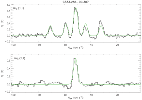
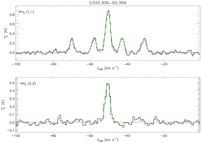
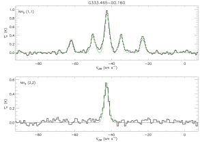
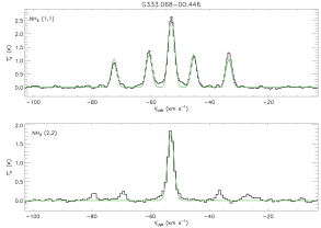
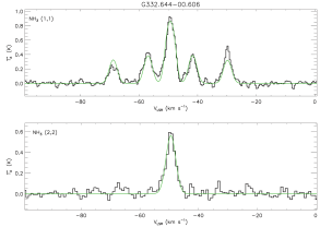
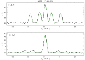
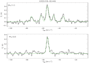
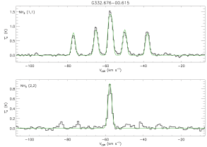
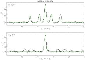
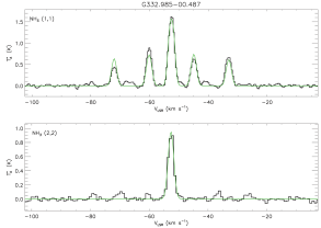
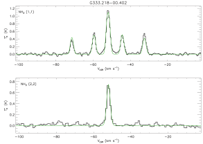
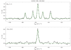
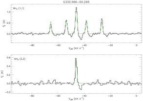
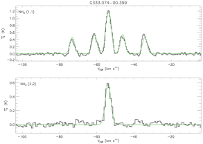
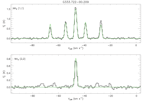
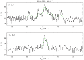
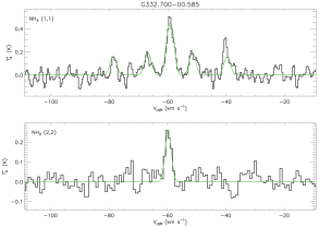
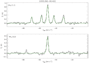
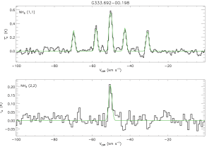
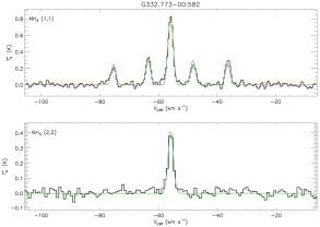
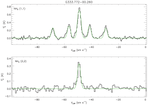
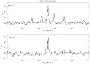
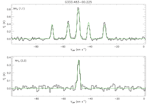
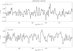
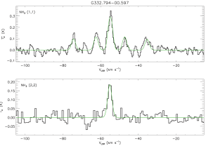
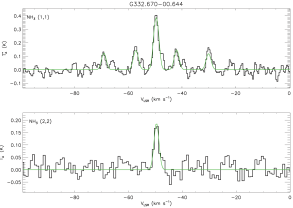
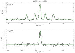
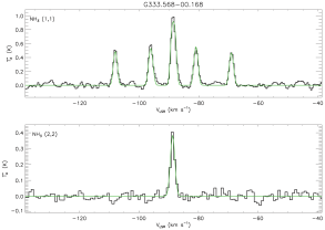
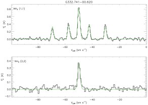
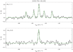
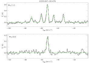
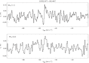
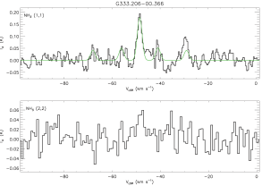
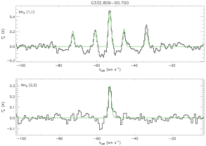
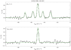
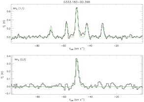
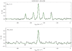
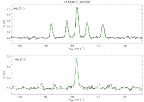
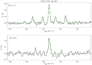
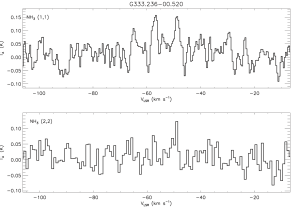
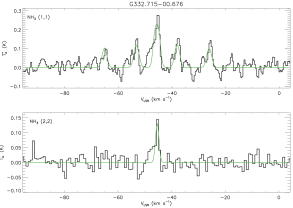
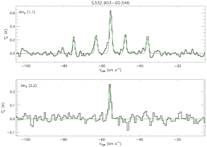
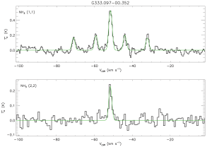
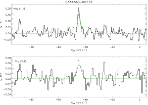
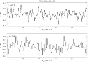
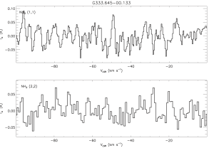
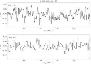
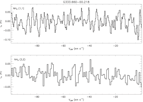
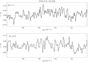
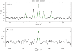
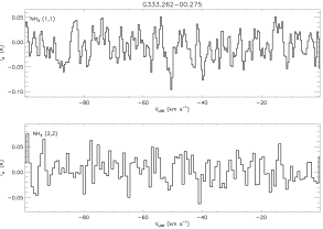
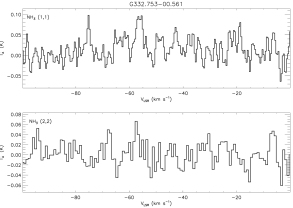
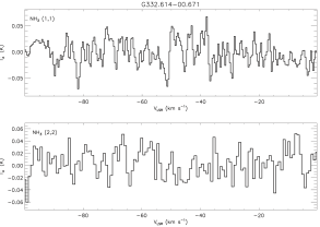
The NH3 (1,1) and (2,2) observations were reduced using the ATNF Spectral Analysis Package (asap) and the graphical interface developed by Cormac Purcell (QuickData.py). The NH3 (3,3), if detected, will be used in future work to constrain the temperatures with large uncertainties. The individual on-off scans were subtracted to remove sky emission and visually inspected to identify and remove poor data. Where necessary a low-order polynomial was fitted to the channels free of emission and subtracted to remove baseline anomalies. The remaining scans were combined to produce a single spectrum for both transitions at each observed position. Hanning smoothing was used to improve the signal to noise of these spectra, which reduced the spectral resolution by a factor of 2. An example of the emission detected in a variety of environments within the G333 GMC are shown in Fig. 2 with the full selection available in Fig. B.

Figure 2: Infrared composite images centred on the peak SIMBA dust clump (left) with accompanying NH₃ emission (right) detected towards a variety of environments within the G333 GMC. Spitzer 4.5 and 8.0 ${\rm\mu m}$, and Herschel 160 ${\rm\mu m}$ are shown in blue, green and red, respectively. The SIMBA dust contours have been set to 0.1, 0.2, 0.5, 1, 1.5, 2.5, 5, 10, 15, 25 and 35 mJy beam^-1. H2O  masers are identified by blue circles. Class I CH3OH  masers are identified by unfilled (44.07 GHz) and filled (95.1 GHz) blue diamonds. Class II CH3OH  masers are identified by unfilled (6.7 GHz) and filled (12.2 GHz) green triangles. OH masers are identified by unfilled (1665/1667/1720 MHz) and filled (6.035 GHz) red squares. Each sub-image is centred on the peak dust emission found within that clump and emphasised by a pink plus sign. The plot showing the NH3 (1,1) and (2,2) spectra are presented on the upper and lower panels, respectively. The model fits to the data are shown in green. The full version of this figure is available in Fig. A and Fig. B, for the infrared composites and spectra, respectively.

2.3 Cool dust from the Herschel Space Observatory

The G333 GMC was observed by Herschel (Pilbratt et al., 2010) with the PACS (Poglitsch et al., 2010) and SPIRE (Griffin et al., 2010) instruments in Parallel mode at 70, 160, 250, 350 and 500 ${\rm\mu m}$ as part of the Open Time Key Programme “Hi-Gal” (PI: S. Molinari; Molinari et al. 2010). The observations comprised of a scan and cross-scan of two 2^∘ fields (field 332.0 with obsid: 1342204046/47 and field 334.0 with obsid: 1342204054/55) taken at a scan speed of 60 arcsec s^-1. These observations were reduced in the Herschel Interactive Processing Environment (HIPE; Ott 2010) to Level 1 (basic calibrated data product), then exported to the scanamorphos map-making software to create a mosaic of the G333 GMC (Roussel, 2013). The pixel size of the final mosaic was 6.4 arcsec per pixel at 160 ${\rm\mu m}$ (equivalent to the instrument native pixel sizes in the red band) was chosen to decrease the low redundancy of the parallel mode scans (due to the high scan speed) and reduce the effect of correlated noise in the final image.

3 RESULTS AND DERIVED PARAMETERS

We derive masses for the clumps from their integrated flux densities at 1.2-mm under the assumption that the clump is optically thin at this wavelength. The dust mass opacity is also quite uncertain, being based on emission models or laboratory dust measurements that may not reflect the actual material we observe. Each clump identified will be used as a mask and aided by a temperature derived from the NH3 observations, accurate abundances will be derived within the clump region for comparing different molecular transitions at 3-mm. For this paper, the peak position within each clump was used to target the NH3 (1,1) and (2,2) observations. We report the results of the NH3 observations and temperature calculations in this paper and will discuss the multi-molecular line abundances in a later paper.

Table 1:  The parameters of the 63 SIMBA 1.2-mm dust clumps identified with clumpfind. The clumpfind number is listed in Column 1, followed by the identifier for each source using the Galactic longitude and latitude designation for the peak pixel in Column 2. Columns 3 and 4 list the coordinates for the clump centroid. The peak flux, radii and total flux within the clumps is found in Columns 5, 6 and 7. Column 8 lists the nearby ($<$ 30 arcsec) infrared and maser associations for each clump, with the number denoting the quantity. The presence of a ‘n’, ‘s’, or ‘p’ denotes Spitzer 3.6, 4.5 or 8.0 ${\rm\mu m}$ emission (Benjamin et al., 2003; Churchwell et al., 2009; Spitzer Science, 2009). The presence of an ‘h’ denotes the presence of a Herschel 160 ${\rm\mu m}$ source. The presence of an ‘o’ denotes an OH maser, an ‘M₁’ denotes a 44.07 GHz Class I CH3OH maser , an ‘M₂’ denotes a 95.1 GHz Class I methanol maser, an ‘m₁’ denotes a 6.7 GHz Class II CH3OH maser, an ‘m₂’ denotes a 12.2 GHz Class II CH3OH maser and a ‘w’ denotes a H2O  maser. If an RMS object was within 30 arcsec of the SIMBA dust peak, then its type is listed in Column 9. Column 10 identifies whether the clump has been classified, via Spitzer 8.0 ${\rm\mu m}$ GLIMPSE emission, as IR-bright or IR-faint. Column 11 identifies which region the clump has been allocated to (see §4.3 for more details).

ID	Clump name	Clump centroid		Peak	Radius	Integrated	Associations†	RMS Type	IR Type	Region
		RA [J2000]	Dec [J2000]	[Jy beam-1]	[pc]	[Jy]
01	G333.604$-$0.210	16:22:08.5	-50:05:53	49.4	0.53	950.8	2wo1,2M2	Hii region	IR-bright	A
02	G332.826$-$0.547	16:20:09.6	-50:53:09	15.5	0.46	263.7	2wo1m1b	Hii region/YSO	IR-bright	C
03	G333.136$-$0.431	16:21:00.8	-50:35:13	14.5	0.55	409.5	nso1,2M2m1	Hii region	IR-bright	B
04	G333.286$-$0.387	16:21:30.3	-50:26:48	09.6	0.49	198.1	nsw	Hii region	IR-bright	B
05	G333.309$-$0.369	16:21:31.4	-50:24:42	06.1	0.80	263.5	ns	Diffuse Hii region	IR-bright	B
06	G333.465$-$0.160	16:21:19.4	-50:09:32	05.6	0.43	095.1	nspwo1M1m1	$\cdots$	IR-bright	A
07	G333.068$-$0.446	16:20:48.6	-50:38:37	05.0	0.49	099.3	nso1,2	YSO	IR-bright	B
08	G332.644$-$0.606	16:19:36.2	-51:03:10	04.6	0.64	173.6	ns	Diffuse Hii region	IR-bright	C
09	G333.127$-$0.564	16:21:35.2	-50:41:15	03.9	0.48	087.4	nsp2o1M1	$\cdots$	IR-faint	B
10	G332.691$-$0.612	16:19:51.6	-51:01:26	02.9	0.43	063.2	nsph	$\cdots$	IR-bright	C
11	G333.018$-$0.449	16:20:37.9	-50:41:22	02.2	0.69	067.1	nshw	Diffuse Hii region	IR-bright	B
12	G332.676$-$0.615	16:19:46.6	-51:02:15	02.1	0.38	038.6	ns	$\cdots$	IR-faint	C
13	G333.524$-$0.272	16:22:02.7	-50:11:42	01.6	0.38	034.0	nsp	$\cdots$	IR-faint	A
14	G332.985$-$0.487	16:20:36.6	-50:44:09	01.5	0.45	039.1	nsm1	YSO	IR-bright	B
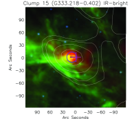
15	G333.218$-$0.402	16:21:17.0	-50:30:15	01.5	0.33	027.9	nspw	$\cdots$	IR-bright	B
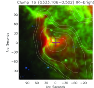
16	G333.106$-$0.502	16:21:13.6	-50:39:42	01.4	0.59	060.1	nspm1	YSO	IR-bright	B
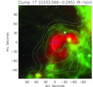
17	G333.566$-$0.295	16:22:20.2	-50:11:22	01.3	0.52	051.6	nsp	$\cdots$	IR-faint	A
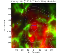
18	G333.074$-$0.399	16:20:37.1	-50:36:41	01.3	0.61	056.8	nsp	$\cdots$	IR-faint	B
19	G333.722$-$0.209	16:22:38.3	-50:00:43	01.2	0.32	023.4	nsph	$\cdots$	IR-bright	A
20	G332.585$-$0.559	16:19:08.3	-51:03:50	01.2	0.43	029.8	nsp	YSO	IR-bright	C
21	G333.006$-$0.437	16:20:27.7	-50:40:56	01.2	0.41	030.0	nspm1	Diffuse Hii region	IR-bright	B
22	G332.700$-$0.585	16:19:45.7	-51:00:14	01.0	0.30	016.5	nspm1	YSO and Hii region	IR-bright	C
23	G333.292$-$0.422	16:21:43.1	-50:27:34	00.9	0.63	041.8	nsp	$\cdots$	IR-faint	B
24	G333.692$-$0.198	16:22:30.1	-50:01:32	00.9	0.40	024.7	ns	$\cdots$	IR-faint	A
25	G332.773$-$0.582	16:20:04.3	-50:57:03	00.9	0.36	017.0	nsp	$\cdots$	IR-faint	C
26	G333.772$-$0.260	16:23:05.2	-50:00:40	00.8	0.31	015.8	nsp	$\cdots$	IR-faint	A
27	G333.539$-$0.245	16:21:59.6	-50:10:03	00.8	0.26	015.2	nsp	$\cdots$	IR-faint	A
28	G333.483$-$0.225	16:21:41.6	-50:11:59	00.8	0.62	029.7	nsp	$\cdots$	IR-faint	A
29	G333.633$-$0.257	16:22:25.9	-50:06:11	00.8	0.50	029.0	ns	YSO	IR-faint	A
30	G333.038$-$0.405	16:20:27.4	-50:38:16	00.7	0.43	023.3	ns	$\cdots$	IR-faint	B
31	G332.794$-$0.597	16:20:14.9	-50:56:28	00.7	0.24	010.8	nsp	$\cdots$	IR-bright	C
32	G332.670$-$0.644	16:19:54.6	-51:03:39	00.7	0.44	021.0	nsp	$\cdots$	IR-faint	C
33	G333.012$-$0.520	16:20:51.8	-50:44:01	00.7	0.43	017.3	nsp	$\cdots$	IR-faint	B
34	G333.568$-$0.168	16:21:47.8	-50:05:36	00.7	0.43	020.4	nsp	$\cdots$	IR-faint	A
35	G332.741$-$0.620	16:20:03.9	-50:59:52	00.7	0.42	016.0	nsphwM1m1,2o1	$\cdots$	IR-faint	C
36	G333.754$-$0.230	16:22:53.0	-50:00:06	00.7	0.16	007.7	nspm1h	YSO	IR-faint	A
37	G333.171$-$0.431	16:21:13.0	-50:33:44	00.6	0.31	010.9	nsp$\cdots$	$\cdots$	IR-faint	B
38	G333.681$-$0.257	16:22:41.5	-50:04:44	00.6	0.47	018.2	ns	$\cdots$	IR-faint	A
39	G333.642$-$0.106	16:21:51.3	-49:59:44	00.6	0.40	016.5	nsph	$\cdots$	IR-bright	A
40	G333.047$-$0.479	16:20:50.2	-50:40:40	00.6	0.40	016.6	nsp	$\cdots$	IR-faint	B
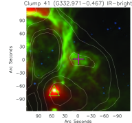
41	G332.971$-$0.467	16:20:27.0	-50:43:47	00.6	0.41	020.1	ns	$\cdots$	IR-bright	B
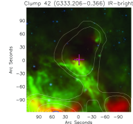
42	G333.206$-$0.366	16:21:01.9	-50:29:08	00.5	0.35	013.5	nsp	$\cdots$	IR-bright	B
43	G332.809$-$0.700	16:20:46.9	-50:59:57	00.5	0.18	006.8	nspM1,2	$\cdots$	IR-bright	C
44	G332.558$-$0.591	16:19:08.9	-51:06:07	00.5	0.20	007.2	nsp	$\cdots$	IR-bright	C
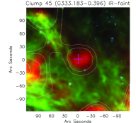
45	G333.183$-$0.396	16:21:05.2	-50:31:34	00.5	0.10	005.0	nsp	$\cdots$	IR-faint	B
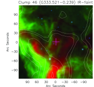
46	G333.521$-$0.239	16:21:53.0	-50:10:48	00.5	0.21	007.3	nsp	$\cdots$	IR-faint	A
47	G333.074$-$0.558	16:21:19.6	-50:42:48	00.4	0.31	008.1	nsph	$\cdots$	IR-bright	B
48	G332.759$-$0.467	16:19:29.4	-50:52:27	00.4	0.12	005.1	ns	$\cdots$	IR-faint	C
49	G333.236$-$0.520	16:21:51.7	-50:34:26	00.4	0.45	012.6	nsp	$\cdots$	IR-bright	B
50	G332.715$-$0.676	16:20:13.4	-51:02:50	00.4	0.31	008.7	ns	$\cdots$	IR-faint	C
51	G332.903$-$0.546	16:20:31.3	-50:49:47	00.4	0.21	005.8	nsp	$\cdots$	IR-faint	C
52	G333.097$-$0.352	16:20:30.7	-50:33:20	00.4	0.23	006.2	ns	$\cdots$	IR-bright	B
53	G333.563$-$0.145	16:21:38.7	-50:04:40	00.3	0.31	006.1	ns	$\cdots$	IR-faint	A
54	G333.636$-$0.165	16:22:04.0	-50:02:37	00.3	0.10	004.2	ns	$\cdots$	IR-faint	A
55	G333.645$-$0.133	16:21:59.0	-50:00:50	00.3	0.30	007.6	nsp	$\cdots$	IR-faint	A
56	G333.657$-$0.133	16:22:01.4	-50:00:01	00.3	0.16	003.8	nsp	$\cdots$	IR-faint	A

Table 1: – continued

ID	Clump name	Clump centroid		Peak	Radius	Sum	Associations†	RMS Type	IR Type	Region
		RA [J2000]	Dec [J2000]	[Jy beam-1]	[pc]	[Jy]
57	G333.660$-$0.218	16:22:25.0	-50:03:43	00.3	0.19	004.7	nsp	$\cdots$	IR-faint	A
58	G333.410$-$0.328	16:21:47.9	-50:19:02	000.3	0.52	010.4	nsph	$\cdots$	IR-bright	A
59	G333.595$-$0.077	16:21:30.0	-50:00:40	000.3	0.32	005.1	nsp	$\cdots$	IR-bright	A
60	G332.894$-$0.567	16:20:32.6	-50:51:16	000.2	0.22	004.4	nsp	$\cdots$	IR-faint	C
61	G333.262$-$0.275	16:20:54.0	-50:23:02	000.2	0.28	004.5	nsp	$\cdots$	IR-bright	B
62	G332.753$-$0.561	16:19:54.0	-50:56:47	000.2	0.23	004.6	nsp	$\cdots$	IR-bright	C
63	G332.614$-$0.671	16:19:43.5	-51:07:40	000.2	0.33	006.0	nsp	$\cdots$	IR-faint	C

$\dagger$ References – Water (22 GHz H2O; Braz & Scalise 1982; Breen et al. 2007, 2010; Walsh et al. 2011), Class I (44.01 GHz; Slysh et al. 1994, Voronkov et al. 2014 and 95.1 GHz; Ellingsen 2005) and II (6.7 GHz; Caswell 1996, 1997, 2009; Caswell et al. 2011; Ellingsen et al. 1996; and 12.2 GHz; Breen et al. 2012) methanol (CH3OH) and hydroxyl (OH; 1665/1667/1720 MHz; Caswell, Haynes, & Goss 1980; Caswell, Vaile, & Forster 1995; Caswell 1998 and 6.035 GHz; Caswell 1997) masers.

3.1 Clump parameters

The parameters of the 63 SIMBA 1.2-mm dust clumps identified with clumpfind can be found in Table 1. The clumpfind number is listed in Column 1, followed by the identifier for each source using the Galactic longitude and latitude designation for the peak pixel in Column 2. Columns 3 and 4 list the coordinates for the clump centroid. We find that the peak of the dust emission correlates poorly with the centroid of the emission, with a maximum deviation of 39.5 arcsec ($\sim$1.3 convolved SIMBA beam). Since the size and shapes of clumps can differ when identified with different algorithms, we have performed our NH3 observations towards the peak dust emission within each clump. The peak and integrated flux (in Jy beam^-1 and Jy, respectively) within the clumps is found in Columns 5 and 7. CUPID outputs the pixel size of the clumps projected onto the equatorial plane, so the average projected values were then converted into parsecs by assuming a distance of 3.6 kpc (Lockman, 1979) and are displayed in Column 6. Column 8 lists the nearby ($<$ 30 arcsec) infrared and maser associations (see §4.1 or Table 1 caption for further information). If there is a nearby ($<$ 30 arcsec) RMS object, then its type is listed in Column 9. Column 10 identifies whether the clump has been classified, via Spitzer GLIMPSE 8.0 ${\rm\mu m}$ emission, as IR-bright or IR-faint. Column 11 identifies which region the clump has been allocated to (see §4.3).

The distribution of the clumps throughout the G333 GMC can be seen in Fig. 1. A sample of the dust clumps and their accompanying NH3 (1,1) and (2,2) emission and Gaussian fits, where possible, can be seen in Fig. 2, with the full version available in Fig. A and Fig. B, for the infrared composites and spectra, respectively.

3.2 Derivation of physical parameters

Table 2: Summary of calculated physical parameters.

Parameter	Mean	1$\sigma$	Min	Max
$T_{\rm{kin}}$[K]	18.1$\pm$0.5	3.6	12.5	35.3
$T_{\rm{rot}}$[K]	22.0$\pm$1.0	7.4	13.6	163.6†
Log[N(NH3)] [cm-2]	15.9$\pm$2.3	0.24	15.3	16.6
Log[n(NH3)] [$\times 10^{5}$ cm-3]	4.5$\pm$0.4	2.8	0.7	16.0
NH3 (1,1) $v_{\rm{LSR}}$ [km s-1]	-52.9$\pm$1.1	8.1	-88.5†	-42.57
NH3 (1,1) $\Delta$V [km s-1]	2.2$\pm$0.9	0.87	1.1	4.5
$\tau_{(1,1)}$	1.9$\pm$0.1	0.86	0.16	3.76
NH3 (2,2) $v_{\rm{LSR}}$[km s-1]	-53.1$\pm$1.2	8.2	-88.7†	-42.8
NH3 (2,2) $\Delta$V [km s-1]	2.7$\pm$0.4	1.0	1.3	6.0
Log(Clump mass) [M⊙]	3.37$\pm$2.61	3.45	2.44	4.12
Log(Virial mass) [M⊙]	2.99$\pm$2.18	3.03	2.03	3.68

^†These values are outliers and their corresponding clumps and physical parameters have been excluded from §4.1.1 onwards. The next highest $T_{\rm{kin}}$ is Clump 21 (G333.006$-$0.437) with $T_{\rm{kin}}$=35.6 K.

Table 3: Summary of physical parameters calculated following §3.2. NH3 (1,1) non-detections with a T${}_{\rm{A}}^{*}<0.1\,\mathrm{K}$ have been excluded.

						NH3 (1,1)				NH3 (2,2)			Log(Mass)		Spectral
ID	Clump Name	$T_{\rm{rot}}$	$T_{\rm{kin}}$	Log[$N({\rm{NH_{3}}})$]	Log[n(H2)]	T${}_{\rm{A}}^{*}$	$v_{\rm{LSR}}$	$\Delta$V	$\tau_{\rm{(m,1,1)}}$	T${}_{\rm{A}}^{*}$	$v_{\rm{LSR}}$	$\Delta$V	Clump	Virial	features†
		[K]	[K]	[cm-2]	[cm-3]	[K]	[km s-1]	[km s-1]		[K]	[km s-1]	[km s-1]	[M⊙]	[M⊙]
01	G333.604$-$0.210	$\cdots$	$\cdots$	$\cdots$	$\cdots$	$<$0.20	$\cdots$	$\cdots$	$\cdots$	$\cdots$	$\cdots$	$\cdots$	$\cdots$	$\cdots$	Aa
02	G332.826$-$0.547	22.0	28.4	16.2	5.75	0.9	$-$57.62	4.50	1.16	0.6	$-$57.16	5.96	3.99	3.62	Hbhgb
03	G333.136$-$0.431	23.8	31.9	15.5	4.97	1.1	$-$53.56	4.45	0.25	0.7	$-$53.79	4.23	4.12	3.68	HABhgab
04	G333.286$-$0.387	22.5	29.2	16.1	5.62	0.9	$-$51.35	2.87	1.52	0.7	$-$51.46	3.50	3.85	3.25	Hbhgb
05	G333.309$-$0.369	20.5	25.5	15.8	5.11	0.9	$-$50.29	2.62	0.85	0.5	$-$50.36	3.10	4.04	3.39	Hg
06	G333.465$-$0.160	19.8	24.4	16.0	5.58	0.9	$-$42.57	2.62	1.38	0.5	$-$42.79	3.10	3.62	3.13	Hg
07	G333.068$-$0.446	20.6	25.7	16.1	5.62	2.5	$-$53.01	2.02	2.25	1.8	$-$53.12	2.66	3.62	2.95	Hhg
08	G332.644$-$0.606	20.1	24.9	16.1	5.50	0.9	$-$49.30	3.01	1.64	0.6	$-$49.43	3.93	3.87	3.41	Hbgb
09	G333.127$-$0.564	17.3	20.3	16.5	6.03	1.6	$-$57.17	3.26	3.76	1.1	$-$57.49	4.31	3.69	3.35	Hbhgb
10	G332.691$-$0.612	18.3	22.0	16.2	5.78	0.6	$-$47.89	2.68	2.51	0.4	$-$47.98	3.23	3.51	3.13	Hbhgb
11	G333.018$-$0.449	25.6	35.6	16.1	5.47	0.4	$-$54.34	3.08	1.29	0.3	$-$54.52	3.25	3.27	3.46	Hbg
12	G332.676$-$0.615	16.3	18.8	16.2	5.83	1.4	$-$57.46	1.89	3.51	0.9	$-$57.62	2.40	3.38	2.78	Hhg
13	G333.524$-$0.272	17.3	20.3	16.0	5.63	1.3	$-$49.34	2.15	1.95	0.7	$-$49.45	2.76	3.28	2.90	Hhg
14	G332.985$-$0.487	18.4	22.1	15.9	5.46	1.6	$-$52.56	1.84	1.92	1.0	$-$52.61	2.31	3.29	2.83	Hhg
15	G333.218$-$0.402	20.1	24.8	15.9	5.59	1.1	$-$51.92	1.76	1.86	0.8	$-$52.06	2.29	3.08	2.65	Hhg
16	G333.106$-$0.502	18.1	21.5	16.0	5.44	1.0	$-$56.12	1.95	2.18	0.6	$-$56.16	2.69	3.50	3.00	Hhg
17	G333.566$-$0.295	15.1	17.1	15.9	5.39	1.1	$-$46.09	1.05	3.27	0.6	$-$46.12	1.34	3.57	2.41	Hahga
18	G333.074$-$0.558	15.9	18.2	16.0	5.42	1.0	$-$55.77	1.74	2.75	0.6	$-$55.95	2.30	3.52	3.31	Hg
19	G333.722$-$0.209	15.6	17.8	16.0	5.70	1.5	$-$46.58	1.41	2.85	0.8	$-$46.69	1.92	3.20	2.46	Hhg
20	G332.585$-$0.559	15.6	17.8	16.0	5.58	0.8	$-$50.99	1.47	2.80	0.4	$-$51.03	2.07	3.30	2.61	Hhg
21	G333.006$-$0.437	35.3	63.6	16.6	6.20	0.2	$-$56.20	4.46	1.80	0.2	$-$55.85	5.17	2.64	3.56	Hbgb
22	G332.700$-$0.585	19.1	23.2	15.9	5.63	0.5	$-$59.15	2.40	1.46	0.3	$-$59.76	2.46	2.89	2.88	Hbg
23	G333.292$-$0.422	18.0	21.4	15.9	5.31	0.9	$-$49.94	1.96	1.56	0.5	$-$49.95	2.50	3.34	3.03	Hg*
24	G333.692$-$0.198	12.5	13.6	16.0	5.61	0.6	$-$50.37	1.25	3.53	0.2	$-$50.36	1.95	3.39	2.44	Hg
25	G332.773$-$0.582	18.7	22.6	15.6	5.25	0.8	$-$55.86	1.72	0.95	0.4	$-$55.92	2.12	2.92	2.68	Hg
26	G333.772$-$0.260	16.6	19.3	15.9	5.62	0.7	$-$48.95	2.43	1.51	0.3	$-$49.02	2.74	2.98	2.91	Hg
27	G333.539$-$0.245	16.5	19.2	15.7	5.49	0.6	$-$48.20	1.39	1.51	0.3	$-$48.32	1.64	2.97	2.35	Hbgb
28	G333.483$-$0.225	14.3	16.0	16.0	5.42	0.8	$-$48.58	1.47	2.89	0.4	$-$48.62	1.99	3.36	2.77	Hg
30	G333.038$-$0.405	17.5	20.6	16.3	5.88	0.3	$-$51.75	4.41	1.85	0.2	$-$52.96	5.49	3.03	2.74	Hbgb
31	G332.794$-$0.597	20.7	26.0	15.9	5.73	0.3	$-$54.89	2.41	1.19	0.2	$-$55.10	2.71	2.65	2.78	Hbgb
32	G332.670$-$0.644	18.0	21.5	15.7	5.27	0.4	$-$49.58	1.96	1.01	0.2	$-$49.58	2.15	3.04	2.89	Hbb
33	G333.012$-$0.520	16.9	19.7	15.8	5.38	0.8	$-$52.94	2.25	1.18	0.4	$-$52.94	2.41	3.01	2.99	Hg
34	G333.568$-$0.168	13.1	14.3	16.0	5.58	0.9	$-$88.53	1.29	3.46	0.4	$-$88.69	1.81	3.27	2.50	Hg
35	G332.741$-$0.620	15.4	17.6	15.8	5.39	0.8	$-$49.81	1.48	2.05	0.4	$-$49.88	2.10	3.04	2.60	Hg
36	G333.754$-$0.230	16.0	18.4	16.0	6.01	0.6	$-$49.70	1.69	2.70	0.3	$-$49.96	2.35	2.69	2.30	Hg
37	G333.171$-$0.431	19.3	23.5	16.0	5.72	1.1	$-$51.07	2.51	1.53	0.7	$-$51.07	3.14	2.70	2.93	Hg
38	G333.681$-$0.257	19.4	23.7	15.3	4.84	0.2	$-$47.04	1.11	0.77	0.1	$-$47.69	2.34	2.93	2.39	Hagb
39	G333.642$-$0.106	13.3	14.6	16.1	5.71	0.8	$-$87.95	1.71	3.06	0.3	$-$87.98	2.11	3.17	2.72	Hg
40	G333.047$-$0.479	16.8	19.5	15.8	5.41	0.6	$-$52.55	1.99	1.40	0.3	$-$52.79	2.76	2.99	2.85	Hg
42	G333.206$-$0.366	$<$9.3	$<$9.5	$<$14.0	$<$3.67	0.2	$-$48.49	2.21	0.16	$\cdots$	$\cdots$	$\cdots$	$\cdots$	2.87	H
43	G332.809$-$0.700	17.7	21.0	15.8	5.75	0.5	$-$52.98	1.17	2.44	0.3	$-$53.17	1.87	2.56	2.03	Hagb
44	G332.558$-$0.591	19.0	23.0	16.0	5.91	0.7	$-$49.64	2.28	1.93	0.4	$-$49.61	2.49	2.54	2.66	Hg
45	G333.183$-$0.396	17.3	20.4	15.8	6.01	0.7	$-$49.95	1.73	1.70	0.4	$-$49.96	2.57	2.44	2.11	Hg
46	G333.521$-$0.239	16.1	18.5	15.8	5.69	0.9	$-$48.16	1.54	1.79	0.4	$-$48.34	2.04	2.67	2.35	Hg
47	G333.074$-$0.399	17.0	19.8	16.1	5.82	1.2	$-$53.69	2.75	1.80	0.6	$-$53.78	3.44	2.72	2.62	Hhg
48	G332.759$-$0.467	17.0	19.9	15.6	5.73	0.6	$-$52.87	1.82	0.93	0.2	$-$52.80	2.44	2.47	2.25	Hg*
50	G332.715$-$0.676	17.0	19.8	16.0	5.72	0.2	$-$45.64	1.92	2.37	0.1	$-$45.38	1.52	2.68	2.79	Hbgb
51	G332.903$-$0.546	15.0	16.9	15.7	5.59	0.6	$-$55.37	1.15	1.91	0.3	$-$55.61	1.37	2.62	2.09	Hbg
52	G333.097$-$0.352	17.1	20.0	15.6	5.45	0.5	$-$51.60	1.71	1.05	0.2	$-$51.59	1.85	2.55	2.48	Hg
53	G333.563$-$0.145	15.9	18.2	15.4	5.12	0.2	$-$44.76	1.90	0.52	0.1	$-$44.60	4.10	2.58	2.72	Hbgb
60	G332.894$-$0.567	15.2	17.2	15.9	5.77	0.5	$-$56.42	1.67	1.96	0.2	$-$56.40	2.07	2.49	2.44	Hg

$\dagger$ The presence of a ‘H’ denotes a NH3 (1,1) hyperfine, ‘A/a’ denotes an absorption feature, ‘B/b’ denotes a blended spectra, ‘g’ denotes a Gaussian was fit to the NH3 (2,2), ‘hg’ denotes that a NH3 (2,2) hyperfine structure could be seen but since the signal-to-noise was below 3$\sigma$, a Gaussian was used to model the fit, and ‘g*’ denotes a NH3 (2,2) characteristic not included in any of the other cases (see §3.2 for further details).

The spectra presented here are calibrated to the corrected antenna temperature scale ($T_{\rm A}^{*}$) and, since the main beam efficiency has not been well determined at this frequency for the 70-m Tidbinbilla radio telescope, we do not convert these to the telescope-independent main-beam temperature scale ($T_{\rm mb}$). However, all our analysis relies on the ratio of the two ammonia transitions, which are essentially independent of calibration as they probe the same volume of gas, so the choice of temperature scale is not important.

We have followed the same fitting routine as described in Urquhart et al. (2011) and include an overview as follows. For the sources with a detectable NH3 (1,1) hyperfine structure ($\sim$75 per cent), we simultaneously fit all 18 hyperfine components and derive the optical depth and FWHM. For the remaining NH3 (1,1) sources and all the NH3 (2,2) sources, a single Gaussian profile was fitted to the main line to obtain a corrected antenna temperature. The NH3 (1,1) and (2,2) FWHM were obtained for all sources by fitting the hyperfine components of their spectra with their respective main line emission in order to remove the effect of line broadening due to the optical depth. An example of the resulting fits are shown in Fig. 2 and the full selection of reduced NH3 (1,1) and (2,2) inversion spectra and the resulting fits can be seen in Fig. B. Emission from the ammonia inversion transition is detected towards 50 (79 per cent) and 49 (78 per cent) of the 63 SIMBA 1.2-mm dust continuum sources, for NH3 (1,1) and (2,2), respectively. There were 13 (21 per cent) clumps without any detectable NH3. We present a summary of the detection rates in Table 2. The standard error of the mean ($s/\sqrt{n}$) is included with the mean. The results of the calculations and spectral fits are given in Table 3. The presence of a ‘H’ denotes a NH3 (1,1) hyperfine, ‘g’ denotes a Gaussian was fit to the NH3 (2,2), and ‘hg’ denotes that a NH3 (2,2) hyperfine structure could be seen but since the signal-to-noise was below 3$\sigma$, a Gaussian was used to model the fit. For two sources, Clumps 23 (G333.292$-$0.422) and 48 (G332.759$-$0.467), a ‘g*’ is used to indicate that the clump has NH3 (2,2) emission at the G333 $v_{\rm{LSR}}$ as well as at -76 km s^-1 and -69 km s^-1, respectively. Features associated with the NH3 (1,1) and (2,2) were shown with an upper and lower case, respectively: ‘A/a’ denotes an absorption feature and ‘B/b’ denotes a blended spectra.

In this section we will describe the method used to determine the physical properties of the millimetre clumps identified within the G333 GMC. The fitted ($v_{\rm{LSR}}$, FWHM) and calculated (optical depth and corrected antenna temperatures) parameters are presented in Table 3. The distribution of various derived parameters are shown in Fig. 3. The uncertainties in the detection rates have been calculated using binomial statistics.

3.2.1 Optical depth, $\tau$

The total optical depth of the NH3 transition, $\tau_{\rm{(1,1)}}$, was obtained numerically from the ratio of the satellite to main line intensity of the hyperfine fits described in §2.2 (Ho & Townes, 1983):

$$\frac{\Delta T^{*}_{a}\left(J,K,m\right)}{\Delta T^{*}_{a}\left(J,K,s\right)}=\frac{1-e^{-\tau\left(J,K,m\right)}}{1-e^{-\alpha\tau\left(J,K,m\right)}}$$ (1)

where J and K are the principal quantum numbers corresponding to the total angular momentum and its projection along the molecular axis, $\Delta T^{*}_{a}$ is the observed brightness temperature, m and s refer to the main and satellite hyperfine components, $\tau$ is the optical depth, and $\alpha$ is the line intensity ratio of the satellite-to-main line [$\alpha$ = 0.28 and 0.22 for the (1,1) satellites]. In using this equation, we have assumed that the hyperfine components have the same beam-filling factor and excitation temperature. This is an acceptable assumption as the energy separations and probability of special excitation mechanisms that differentiate between the hyperfine components are small.

3.2.2 Rotation temperature, $T_{\rm{rot}}$

The rotational temperature, $T_{\rm{rot}}$, for the NH3 (1,1) and (2,2) transitions can be calculated using the main line intensities and the NH3 (1,1) main quadrupole transition optical depth (Ho & Townes, 1983):

$$T_{\mathrm{rot}}=\frac{-T_{0}}{\ln\left\{\frac{-0.282}{\tau_{(1,1,m)}}\ln\left[1-\frac{\Delta T_{\mathrm{a}}^{*}\left(2,2\right)}{\Delta T_{\mathrm{a}}^{*}\left(1,1,m\right)}\left(1-\mathrm{e}^{-\tau_{(}1,1,m)}\right)\right]\right\}}~{}[{\rm{K}}]$$ (2)

where $T_{0}=\frac{E_{(2,2)}-E_{(1,1)}}{k_{B}}\approx 41.5$ K is the temperature of the energy difference between the NH3 (1,1) and (2,2) levels, $T_{\mathrm{a}}^{*}$ is the observed brightness temperature and $\tau$ is the optical depth. Fourteen clumps did not have a detectable NH3 (2,2) emission, whilst thirteen clumps did not have a detectable NH3 (1,1) emission. Clump 42 (G333.206$-$0.366), has a detectable NH3 (1,1), using the root mean square of the (2,2) band, we calculate an upper limit of 9.3 K and 9.5 K for $T_{\rm{rot}}$ and $T_{\rm{kin}}$, respectively. For all other clumps (1, 29, 41, 49, 54-59, 61-63), fitting the NH3 (1,1) and/or (2,2) spectra was not possible so no physical parameters have been calculated for these clumps.

3.2.3 Kinetic temperature, $T_{\rm{kin}}$

For $T_{\rm{kin}}$$<$ $T_{0}\approx 41.5$ K, an empirical relationship between the rotational and kinetic temperature can be calculated (Swift et al., 2005):

$$T_{\mathrm{rot}}=\frac{T_{\mathrm{kin}}}{1+\frac{T_{\mathrm{kin}}}{T_{0}}\ln\left[1+0.6\times\exp\left(\frac{-15.7}{T_{\mathrm{kin}}}\right)\right]}~{}[{\rm{K}}]$$ (3)

however, at high kinetic temperatures this expression underestimates the $T_{\rm{rot}}$. From the original sample of 63 SIMBA clumps, 49 had detectable NH3 (2,2) emission. However, one clump displays a $T_{\rm{rot}}$ which has large uncertainties [Clump 21 (G333.006$-$0.437)].

3.2.4 Column density, N

By assuming that all hyperfine lines have the same excitation temperature and that the excitation conditions are homogeneous along the beam, then the column density at a given transition (e.g. N_(1,1)) can be written (Mangum et al., 1992):

$$N_{\rm{(1,1)}}=6.60\times 10^{14}\Delta v_{\rm{(1,1)}}\tau_{\rm{(1,1)}}\frac{T_{\mathrm{rot}}}{\nu_{\rm{(1,1)}}}~{}~{}[{\rm{cm}}^{-2}]$$ (4)

where $\Delta v_{\rm{(1,1)}}$ is the FWHM of the NH3 (1,1) transition in km s^-1 and $\nu_{\rm{(1,1)}}$ is the transition frequency in GHz. We estimate the total ammonia column density following (Li, Goldsmith, & Menten, 2003):

$$N_{\rm{NH_{3}}} =N_{\rm{(1,1)}}\left[1+\frac{1}{3}{\rm{exp}}\left(\frac{23.1}{T_{\mathrm{rot}}}\right)+\frac{5}{3}{\rm{exp}}\left(\frac{-41.2}{T_{\mathrm{rot}}}\right)\right.$$

$$\left.+\frac{14}{3}{\rm{exp}}\left(\frac{-99.4}{T_{\mathrm{rot}}}\right)\right]~{}~{}[{\rm{cm}}^{-2}]$$ (5)

3.2.5 Volume density, n

By assuming a fixed NH3/H₂ abundance of 10^-8 (Johnstone et al., 2010), the NH3 volume density, $n$, can be calculated:

$$n=\frac{N}{2R}~{}~{}[{\rm{cm}}^{-3}]$$ (6)

where $N$ is the column density in cm^-2 and $R$ is the clump radius in cm. The mean volume density within the G333 GMC is 4.5 $\times~{}10^{5}$ cm^-3, with a standard deviation of 2.8 $\times~{}10^{5}$ cm^-3.

3.2.6 Clump (M_clump) and virial (M_virial) masses

Assuming the dust is optically thin and using the $T_{kin}$ derived from NH3, we calculate the clump mass, $M_{clump}$, as (Hildebrand, 1983):

$$M_{clump}=\frac{F_{\nu}D^{2}}{\kappa_{\nu}B_{\nu}\left(T_{kin}\right)}\left[M_{\sun}\right]$$ (7)

where $F_{\nu}$ is the 1.2-mm flux density, $D$ is the distance, $\kappa_{\nu}$ is the dust mass opacity coefficient (Ossenkopf & Henning, 1994) and $B_{\nu}\left(T_{kin}\right)$ is the Planck function at the dust temperature, $T_{kin}$.

Assuming that we have a Gaussian volume density distribution throughout the clump and that the gravitational energy within a clump is balanced by the turbulent energy, we calculate the virial mass, $M_{virial}$, following (Protheroe et al., 2008):

$$M_{virial}=444\left(\frac{R}{1\,\mathrm{pc}}\right)\left(\frac{v_{\mathrm{FWHM}}}{1\,\mathrm{kms}^{-1}}\right)^{2}\left[M_{\sun}\right]$$ (8)

where $R$ is the radius of the SIMBA 1.2-mm dust clump and $v_{\mathrm{FWHM}}$ is the FWHM.

Figure 3: Distribution of the parameters from IR-bright (solid blue) and IR-faint (dashed red) clumps. The solid black line indicates the distribution for clumps with detectable NH3 (1,1) and (2,2).

Table 4: Summary of derived parameters for IR-bright and IR-faint clumps.

	IR-bright clumps						IR-faint clumps
Parameter	Number	Mean	1$\sigma$	Median	Min	Max	Number	Mean	1$\sigma$	Median	Min	Max
$T_{\rm{rot}}$ [K]	20	19.6$\pm$0.6	2.6	19.5	15.6	25.6	26	16.6$\pm$0.3	1.5	16.7	12.5	19.4
$T_{\rm{kin}}$ [K]	20	24.2$\pm$1.0	f 4.5	23.8	17.8	35.6	26	19.3$\pm$0.4	2.3	19.4	13.6	23.7
Log[N(NH3)] [cm-2]	20	16.0$\pm$0.04	0.2	16.0	15.5	16.2	26	15.9$\pm$0.05	0.3	15.9	15.3	16.5
Log[n(NH3)] [$\times 10^{2}$ cm-3]	20	5.57$\pm$0.05	0.23	5.61	4.97	5.91	26	5.56$\pm$0.06	0.29	5.60	4.84	6.03
NH3 (1,1) $v_{\rm{LSR}}$ [km s-1]	21	-51.84$\pm$0.82	3.78	-51.92	-59.15	-42.57	26	-50.97$\pm$0.71	3.63	-49.95	-57.46	-44.76
NH3 (1,1) FWHM [km s-1]	21	2.44$\pm$0.19	0.86	2.40	1.17	4.50	26	1.90$\pm$0.14	0.70	1.78	1.05	4.41
$\tau_{(1,1)}$	21	1.64$\pm$0.16	0.74	1.64	0.16	2.85	26	1.96$\pm$0.18	0.90	1.82	0.52	3.76
NH3 (2,2) $v_{\rm{LSR}}$ [km s-1]	20	-52.11$\pm$0.85	3.80	-52.34	-59.76	-42.79	26	-51.11$\pm$0.72	3.68	-49.96	-57.62	-44.60
NH3 (2,2) FWHM [km s-1]	20	2.95$\pm$0.22	0.98	2.70	1.85	5.96	26	2.50$\pm$0.18	0.92	2.35	1.34	5.49
Log($M_{clump}$) [M⊙]	20	3.31$\pm$0.12	0.53	3.30	2.54	4.12	26	2.99$\pm$0.07	0.36	2.99	2.44	3.69
Log($M_{virial}$) [M⊙]	21	2.95$\pm$0.09	0.42	2.88	2.03	3.68	26	2.67$\pm$0.07	0.34	2.73	2.09	3.35

4 ANALYSIS AND DISCUSSION

Figure 4: The distribution of IR-bright (blue pluses) and IR-faint (red pluses) clumps throughout the G333 giant molecular cloud. The clumps excluded as per §4.1.1 are shown as green pluses. The clumps have also been separated into three regions (A, B, C). The positions associated with RCW 106 have been overlaid with black stars (Rodgers et al., 1960).

4.1 Separation into clumps with and without 8 ${\rm\mu m}$ emission

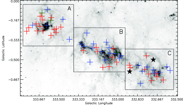
Through visual inspection of Spitzer GLIMPSE 8 ${\rm\mu m}$ emission we separated our sample of 63 SIMBA 1.2-mm clumps into two categories: clumps with (IR-bright) or without (IR-faint) significant 8 ${\rm\mu m}$ emission (Fig. 4), since the 8 ${\rm\mu m}$ band is sensitive to ionised PAH (PAH⁺) emission which is excited by the ultraviolet radiation from high-mass stars in photon dominated regions (PDRs). MIPSGAL 24 ${\rm\mu m}$ emission, which represents heated very small dust grains was not used due to saturation in the 24 ${\rm\mu m}$ band within the G333 GMC.

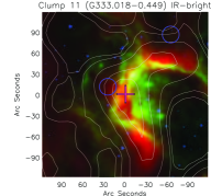
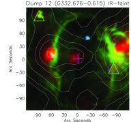
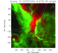
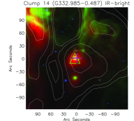
We identified 30 IR-bright and 33 IR-faint clumps. Column 8 of Table 1 lists the nearby ($<$ 30 arcsec) star forming signatures (see table caption for details). The Red MSX Source (RMS) Survey uses a multi-wavelength follow-up to disentangle their colour-selected MSX and 2MASS point sources into stages of star formation (Lumsden et al., 2013). There are RMS objects associated within 30 arcsec of the SIMBA dust peak for 15 of 63 clumps (24 per cent). The type of RMS object is listed in Column 9 of Table 1. Possible types include YSO, Hii region/YSO, Hii region and diffuse Hii region. Masers are known to be signposts for star formation so the water (H2O), Class I and II (6.7 GHz and 12.2 GHz) methanol (CH3OH) and hydroxyl (OH; 1665/1667/1720 MHz and 6.035 GHz) masers have been overlaid to show potential sites of star formation. The different classes of CH3OH masers indicate different pumping mechanisms. Class I CH3OH masers are collisionally pumped and associated with regions with outflows and shocks. Class II CH3OH masers are radiatively pumped and exclusively associated with high-mass star forming regions (Minier et al., 2003; Breen et al., 2013). The infrared (4.5, 8.0, 160 ${\rm\mu m}$) dust emission has also been included to show regions of shocked gas, PDRs, and cool dust, respectively.

We find that our SIMBA dust clumps are associated with a variety of environments within the G333 GMC. Each of our clumps are associated with varying amounts of infrared emission, as seen in Fig. 2 and A. Emission at 8.0 ${\rm\mu m}$ is common, which indicates that the G333 GMC is undergoing star formation, but there are also pockets of 160 ${\rm\mu m}$ emission at sites of cool dust which may show regions where the embedded protostar has not significantly warmed its surroundings. It is known that modelling the spectral energy distribution of the dust can be used to identify clumps at different stages of star formation and that NH3 is a good tracer of the dense cold gas which traces the molecular gas involved in star formation (e.g. Dunham et al. 2011; Urquhart et al. 2011; Wienen et al. 2012). By combining the information from both the NH3 and dust emission for the G333 GMC, we will develop a better understanding of the star formation occurring therein.

4.1.1 Main cloud clumps

From our original sample of 63 SIMBA dust clumps, we have detected NH3 (1,1) towards 50 clumps (79 per cent) and (2,2) towards 49 clumps (78 per cent). No NH3 was detected towards Clump 1 (G333.604-0.210) due to self-absorption against a strong continuum emission generated by the Hii region, RCW 106 (Rodgers et al., 1960). The majority of clumps with no detectable amounts of NH3 are associated with the weakest millimetre continuum sources within the G333 GMC. The NH3 (1,1) and (2,2) detection rates for the IR-bright and IR-faint clumps are not obviously different. Of the 30 IR-bright clumps, 23 (77 per cent) and 22 (73 per cent) of the clumps had detectable NH3 (1,1) and (2,2) emission, respectively. Of the 33 IR-faint clumps, 27 clumps (82 per cent) had both NH3 (1,1) and (2,2) emission.

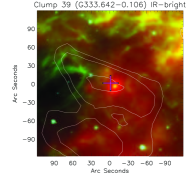
Two clumps (one clump from each category) was identified via NH3 (1,1) velocity information to be outside of the $v_{\rm{LSR}}$ range of the main G333 GMC and are excluded from the analysis in the later portions of this paper unless explicitly included. These clumps are Clump 34 (G333.586$-$0.168) with a $v_{\rm{LSR}}$ of -88.53 km s^-1 (a clump with trace amounts of diffuse 8 ${\rm\mu m}$ emission), and Clump 39 (G333.642$-$0.106) with a $v_{\rm{LSR}}$ of -87.95 km s^-1 (a YSO which has cleared its surrounding Hii region). The $v_{\rm{LSR}}$ for the excluded clumps corresponds with the Norma-Cygnus arm and the included clumps corresponds with the Norma-Cygnus and/or Scutum-Crux arms (fig. 3 of Vallée 2008). At temperatures much greater than 30 K, NH3 (1,1) and (2,2) cannot accurately be used as a temperature probe and any physical parameters using this kinetic temperature calculation would also be inaccurate (Danby et al., 1988; Hill et al., 2010). As Clump 21 (G333.006$-$0.437) had a derived kinetic temperature of 63.6 K, it has been removed from the following analysis. We note that Clump 3 (G333.136$-$0.431) has a $T_{\rm{kin}}$ of 31.9 K and Clump 11 (G333.018$-$0.449) has a $T_{\rm{kin}}$ of 35.6 K, but has been retained for the following analysis.

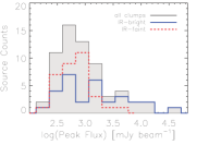
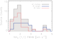
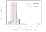
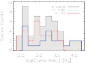
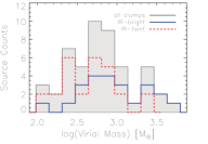
From the original sample of 63 SIMBA 1.2 mm dust clumps, we are left with 29 IR-bright and 31 IR-faint clumps (Table 4). Their distribution (with the excluded three clumps) for the derived parameters is shown in Fig. 3. We note that derived parameters could not be calculated for all clumps due to the non-detection of NH3 (1,1) and/or (2,2). The black shaded histogram shows the total number of clumps with that derived parameter. IR-bright and IR-faint clumps are shown by the solid blue and dashed red line, respectively. The distributions in these histograms generally have skewed Gaussian-like profiles. The kinetic temperature, the FWHM of the NH3 (1,1) transition and the dust and virial masses show that the distribution is skewed in favour of higher values for all these parameters for the IR-bright clumps, while the IR-faint clumps cluster at the lower end. These are not wholly independent parameters, as we have used the same spectrum to measure the FWHM and temperature for the calculations of the virial and clump mass, respectively. However, these histograms show a qualitative difference between the two populations. We investigate these variations further with statistical methods in the next section.

4.2 Importance of accurate kinetic temperatures

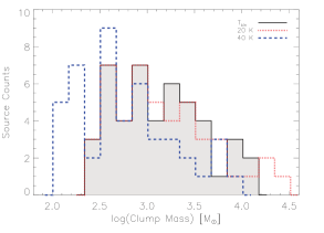
It is common to assume 20 K for isolated clumps and 40 K for Hii regions (e.g. Mookerjea et al. 2004 for the G333 GMC). Since NH3 (1,1) and (2,2) are closely separated ($\Delta\nu\approx 28\,\mathrm{MHz}$), we are able to obtain the $T_{\rm{rot}}$ and $T_{\rm{kin}}$ with the same observation per clump. In Fig. 5, we display the effect that kinetic temperature has on the calculation of clump mass [Eqn. (7)]. We find that clumps with $T_{\rm{kin}}$=20 K are more massive, whereas clumps with $T_{\rm{kin}}$= 40 K are less massive. From the dust mass for clumps derived using $T_{\rm{kin}}$, we found a mean of 2390 M_⊙, a median of 1089 M_⊙, a standard deviation of 2920 M_⊙ and a range between 278–13036 M_⊙. For the masses calculated assuming 40 K, we found a mean of 1285 M_⊙, a median of 483 M_⊙, a standard deviation of 1992 M_⊙ and a range between 105–9951 M_⊙. For the masses calculated using 20 K, we found a mean of 3064 M_⊙, a median of 1151 M_⊙, a standard deviation of 4750 M_⊙ and a range between 251–23723 M_⊙. We find that T=20 K overestimates the mass whereas T=40 K underestimates it. Therefore, an accurate temperature is important for determining if a clump is bound and will collapse onto itself, or if it is unbound and remains a starless core.

Figure 5: The distribution of clump mass as a function of temperature. The solid black line was calculated from the temperature found from NH3, whilst the dotted red and dashed blue were calculated from the assumption of 20 and 40 K, respectively.

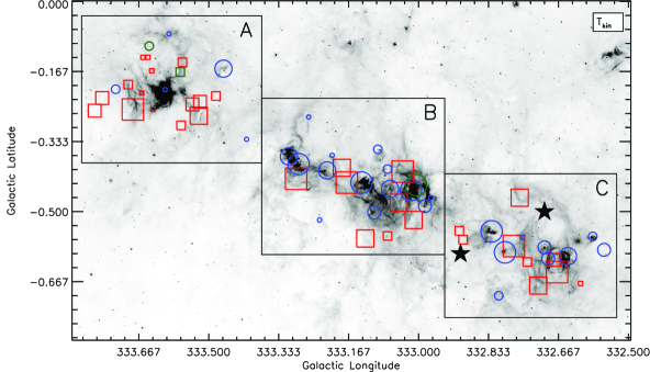
4.3 Variations in physical parameters throughout the cloud

Figure 6: The distribution of the $v_{\rm{LSR}}$ of NH3 (1,1) throughout the G333 giant molecular cloud. Each clump was classified as IR-bright (blue circles) or IR-faint (red squares) clumps using the presence of Spitzer GLIMPSE 8.0 $\mu m$ emission (grey-scale image). The samples were separated into non-detections and detections, with the detections further split into four sub-samples at the 25th, 50th and 75th percentile. The IR-bright and IR-faint clumps which were excluded, as per §4.1.1, are shown as green circles and squares, respectively, and the symbol size for these clumps corresponds with the percentile calculations for the included clumps. The clumps have also been separated into three regions (A, B, C). The positions associated with RCW 106 have been overlaid with black stars (Rodgers et al., 1960).

Figure 7: The distribution of the FWHM of NH3 (1,1) throughout the G333 giant molecular cloud. Each clump was classified as IR-bright (blue circles) or IR-faint (red squares) using the presence of Spitzer GLIMPSE 8.0 $\mu m$ emission (grey-scale image). The samples were separated into non-detections and detections, with the detections further split into four sub-samples at the 25th, 50th and 75th percentile. The IR-bright and IR-faint clumps which were excluded, as per §4.1.1, are shown as green circles and squares, respectively, and the symbol size for these clumps corresponds with the percentile calculations for the included clumps. The clumps have also been separated into three regions (A, B, C). The positions associated with RCW 106 have been overlaid with black stars (Rodgers et al., 1960).

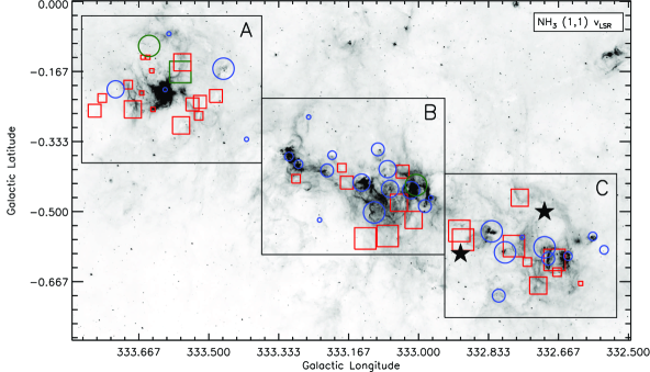
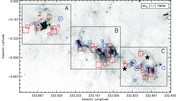
The majority of clumps can be grouped into three regions (A, B, C; Fig. 4) and the distribution of physical parameters throughout the G333 GMC is shown in Table 5 and Fig. 6, 7 and 8. For Fig. 4, each clump was classified as IR-bright (blue pluses) or IR-faint (red pluses) clumps using the presence of Spitzer GLIMPSE 8.0 $\mu m$ emission (grey-scale image). The excluded clumps are shown with green pluses. For the NH3 (1,1) FWHM (Fig. 7) and $T_{\rm{kin}}$ (Fig. 8), the samples were separated into non-detections and detections, with the detections further split into four sub-samples (Q1, Q2, Q3, Q4) at the 25th, 50th and 75th percentile by taking the medians of the NH3 (1,1) FWHM and $T_{\rm{kin}}$, respectively. The NH3 (1,1) $v_{\rm{LSR}}$ was separated in a similar fashion but the absolute difference between the $v_{\rm{LSR}}$ of the G333 GMC ($\sim$50 km s^-1; Bains et al. 2006) and the NH3 (1,1) $v_{\rm{LSR}}$ was used. The values of these subdivisions can be seen in Table 5. The symbol size correlates with the percentile sub-sample, and IR-bright and IR-faint clumps are shown as blue circles and red squares, respectively. The IR-bright and IR-faint clumps which were excluded, as per §4.1.1, are shown as green circles and squares, respectively, and the symbol size for these clumps corresponds with the percentile calculations for the included clumps.

Region A contains one of the brightest infrared sources in the southern Galactic Plane (G333.6$-$0.2; Becklin et al. 1973), however NH3 for the associated Clump 1 (G333.604$-$0.210) was not fit due to NH3 self-absorption, so we were unable to extract any physical parameters from the largest and most active clump within the G333 GMC. It also appears to be surrounded by IR-faint clumps. Region A contains 5 and 15 IR-bright and IR-faint clumps, respectively. This asymmetry could be due to the destructive interaction of the Hii region with the GMC. There are two other Hii regions [G333.6$-$0.1 (Goss & Shaver, 1970) and IRAS 16175-5002 (Ellingsen et al., 1996)] within this region and both are associated with IR-bright clumps. However, only IRAS 16175-5002 has detectable NH3 emission. The $v_{\rm{LSR}}$ of the clumps within Region A does not significantly differ from the $v_{\rm{LSR}}$ of the G333 GMC. However, the two clumps which were excluded, as per §4.1.1, due to having a $v_{\rm{LSR}}$ different to the main G333 cloud, were found in this region.

Region A shows relatively small $v_{\rm{LSR}}$ deviations ($<$ 1.5 km s^-1 from the $v_{\rm{LSR}}$ of the G333 GMC) for IR-faint clumps. However, with over half the included IR-bright clumps showing non-detections (with, at least, one due to NH3 self-absorption), we cannot reliably comment further on the $v_{\rm{LSR}}$ of the IR-bright clumps in Region A. Clump 6 (G333.465$-$0.160) contains the largest NH3 (1,1) FWHM for IR-bright clumps in this region and is associated with the UCHii region, IRAS 16175$-$5002 (e.g. Walsh et al. 1998). However, there are two IR-faint clumps [Clumps 13 (G333.524$-$0.272) and 26 (G333.772$-$0.260)] in the highest percentile. Both of these clumps have an excess of 160 ${\rm\mu m}$ emission with Clump 13 (G333.524$-$0.272) showing possible compression between two expanding 8 ${\rm\mu m}$ bubbles. Most (60 %) of the $T_{\rm{kin}}$ values for IR-bright clumps are non-detections. Half (53 %) of the IR-faint clumps are below the 50th percentile, and a third are non-detections. Clump 13 (G333.524$-$0.272) shows the second highest $T_{\rm{kin}}$ (20.3 K) for the IR-faint clumps and Clump 38 (G333.681$-$0.106) shows the highest (measured) $T_{\rm{kin}}$ (23.7 K) of the region.

Region B appears to be the opposite and contains 14 and 8 IR-bright and IR-faint clumps, respectively. There are three clusters of Hii regions and they correspond with IR-bright clumps; however there are also IR-bright clumps that are not Hii regions. The IR-faint clumps appear to be on the outskirts of Hii regions. The IR-bright clumps in Region B show smaller deviations from the $v_{\rm{LSR}}$ towards the north of the GMC and the clumps with larger deviations clustered towards the south. The IR-faint clumps have larger $v_{\rm{LSR}}$ deviations and are closer to the south. This region shows the largest NH3 (1,1) FWHM for IR-faint clumps, whereas the IR-bright clumps are somewhat equally spaced throughout all quartiles. The majority of high $T_{\rm{kin}}$ appear to be associated with, or adjacent to, the Hii regions, however Clump 9 (G333.127$-$0.564) has a $T_{\rm{kin}}$ of 20.3 K and appears to have excess 160 ${\rm\mu m}$ emission coincident with the 1.2-mm flux peak, and Class I and II CH3OH masers.

Region C also contains multiple Hii regions (including RCW 106) but the number of IR-bright and IR-faint clumps are equal (with 9 clumps in each category). Rodgers et al. (1960) identified two bright areas in RCW 106: one at G332.9$-$0.6 and the other at G333.7$-$0.5, with their extent covering 20 arcmin $\times$ 7 arcmin and 12 arcmin $\times$ 12 arcmin, respectively. This covers the majority of SIMBA clumps within Region C. For Region B and C, we note that the IR-faint clumps are often towards the edge of each region. This suggests that star formation on these scales are propagating outwards from the central and more evolved parts of the regions, which suggests sequentially triggered star formation. Region C has a larger proportion of IR-faint clumps showing larger $v_{\rm{LSR}}$ deviations, with the largest deviations seen towards the boundary of Regions B with C. The largest values for the NH3 (1,1) FWHM are seen towards the IR-bright clumps that are associated with Hii regions. For the IR-faint clumps, the $T_{\rm{kin}}$ tend towards the larger values. Clump 25 (G332.773$-$0.582) and Clump 32 (G332.670$-$0.644) are IR-faint clumps however they show high $T_{\rm{kin}}$ (22.6 and 21.5 K, respectively) but have low values for NH3 (1,1) FWHM (1.72 and 1.96 km s^-1). These clumps are also adjacent to IR-bright clumps so appear to be sites of future or currently unseen star formation.

The 63 clumps within the G333 GMC can be grouped into three regions. The physical parameters throughout the GMC are influenced by the numerous Hii regions. Region A contains the most number of IR-faint clumps (15), whilst Region B contains the most number of IR-bright clumps (14), and Region C contains the same number (nine) of IR-bright and IR-faint clumps. Region A and B contain the most number of NH3 non-detections, with eight and three, respectively. This may be because of the effect that the Hii regions, G333.6$-$0.2 and RCW 106, have on the surrounding molecular gas. Region B contains seven clumps with large (Q4; 2.15$-$4.41 km s^-1) NH3 (1,1) FWHM, whilst both Regions A and C have two each. This could indicate that the Hii regions in Region A and C are sweeping molecular material into Region B. Region A and C have the most clumps with low (Q1; 13.6$-$18.2 K) $T_{\rm{kin}}$, whereas Region B has the warmest [Q3-Q4; 13 clumps with $T_{\rm{kin}}$ above the median (19.4 K)]. Region C also contains the most numbers of clumps with the largest (Q4; 5.37$-$7.46 km s^-1) deviation from the $v_{\rm{LSR}}$ of the G333 GMC.

Figure 8: The distribution of the $T_{\rm{kin}}$ throughout the G333 giant molecular cloud. Each clump was classified as IR-bright (blue circles) or IR-faint (red squares) clumps using the presence of Spitzer GLIMPSE 8.0 $\mu m$ emission (grey-scale image). The samples were separated into non-detections and detections, with the detections further split into four sub-samples at the 25th, 50th and 75th percentile. The IR-bright and IR-faint clumps which were excluded, as per §4.1.1, are shown as green circles and squares, respectively, and the symbol size for these clumps corresponds with the percentile calculations for the included clumps. The clumps have also been separated into three regions (A, B, C). The positions associated with RCW 106 have been overlaid with black stars (Rodgers et al., 1960).

Table 5: Variations in physical parameters within the regions in the G333 GMC. The samples were separated into non-detections and detections, with the detections further split into four sub-samples (Q1, Q2, Q3, Q4) at the 25th, 50th and 75th percentile. The NH3 (1,1) $v_{\rm{LSR}}$ was separated in a similar fashion but the absolute difference between the $v_{\rm{LSR}}$ of the G333 GMC ($\sim$50 km s^-1; Bains et al. 2006) and the NH3 (1,1) $v_{\rm{LSR}}$ was used. Excluded clumps as per §4.1.1 were not used to calculate the quartiles but a + indicates the quartile it would belong to.

	Region
FWHM	A		B		C
$[$km s-1]	IR-bright	IR-faint	IR-bright	IR-faint	IR-bright	IR-faint
2.15–4.41	0	2	03+	4	2	0
1.82–1.99	1	1	2	2	2	4
1.54–1.74	0	2	3	2	2	2
1.11–1.48	01+	05+	3	0	2	2
non-detection	3	5	3	0	1	1
	Region
$T_{\rm{kin}}$	A		B		C
$[$K]	IR-bright	IR-faint	IR-bright	IR-faint	IR-bright	IR-faint
20.6–23.7	0	1	03+	3	2	2
19.5–20.4	1	1	3	4	1	2
18.4–19.3	0	4	2	0	3	1
13.6–18.2	01+	04+	2	1	2	3
non-detection	3	5	4	0	1	1
	Region
NH3 (1,1) $v_{\rm{LSR}}$	A		B		C
$[$km s-1]	IR-bright	IR-faint	IR-bright	IR-faint	IR-bright	IR-faint
5.37–7.46	01+	00+	01+	2	3	4
2.55–5.24	1	3	4	2	0	2
1.05–1.84	0	4	3	2	2	0
0.05–0.66	0	3	3	2	3	2
non-detection	3	5	3	0	1	1
Total	05+	15+	14+	8	9	9

4.4 Correlations of physical parameters

We have calculated the linear Pearson correlation coefficient and the linear fit to test the level of correlation between physical parameters for the IR-bright and IR-faint clumps.

The linear Pearson correlation coefficient, $r$, for different pairs of physical parameters, were found with the correlate function found in IDL. For each $\left(x_{i},y_{i}\right)$ pair, with $i=1,....,N$, $r$ can be written following Press et al. (1992, chap. 14) as:

$$r=\frac{\sum_{i}\left(x_{i}-\bar{x}\right)\left(y_{i}-\bar{y}\right)}{{\sqrt{\sum_{i}\left(x_{i}-\bar{x}\right)^{2}}}{\sqrt{\sum_{i}\left(y_{i}-\bar{y}\right)^{2}}}}$$ (9)

The linear fits between different physical parameters were found with the linfit function found in IDL. It fits a linear model ($y=a+bx$), while minimising the chi-square error statistic. The chi-square error statistic, $\chi^{2}$, can be written following Press et al. (1992, chap. 15) as:

$$\chi^{2}(a,b)=\displaystyle\sum_{i=1}^{N}\left(y_{i}-a-bx_{i}\right)^{2}$$ (10)

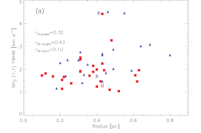
The relationship between clump radius and FWHM can be seen in Fig. 9(a). There is significant scatter in the data, as seen by the medium positive correlation for IR-bright clumps ($r_{\mathrm{IR-bright}}~{}=~{}0.43$) and low positive correlation for IR-faint clumps ($r_{\mathrm{IR-faint}}~{}=~{}0.10$), which shows a poor linear fit to the data. This implies that before the onset of 8 ${\rm\mu m}$ emission, NH3 is not correlated with the physical parameters of the clump but once they become IR-bright, the FWHM has some correlation with 8 ${\rm\mu m}$ emission. There are four clumps with NH3 (1,1) FWHM $\sim$4.5 km s^-1 that deviate from the other clumps. Three of these clumps are IR-bright, however one (Clump 21 G333.006$-$0.437) has been excluded from our analysis as per §4.1.1. Two of the included clumps (Clump 3 G333.136$-$0.431 and Clump 30 G333.038$-$0.405) belong to Region B but one is IR-bright and the other is IR-faint. The third included clump belongs to Region C.

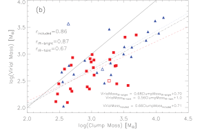
The relationship between the virial and clump mass can be seen in Fig. 9(b). However, the G333 GMC contains numerous Hii regions which have free-free emission which can contribute to the 1.2 mm emission. This may contaminate surrounding clumps resulting in smaller clump masses [Eqn. (7)]. Of these 32 clumps, 72 per cent (23 of 32) were classified as IR-faint clumps. The masses for 14 clumps could not be calculated because no NH3 emission was detected in 12 clumps; the emission profile was too complex, due to self-absorption, for Clump 1 (G333.604$-$0.210); and NH3 (2,2) was not detected in Clump 42 (G333.206$-$0.366). There are high positive correlations for both IR-bright and IR-faint clumps, with $r_{\mathrm{IR-bright}}=0.87$ and $r_{\mathrm{IR-faint}}=0.67$. The three clumps which have been previously excluded in §4.1.1, were included in Fig. 9 as unfilled blue triangles and unfilled red squares to represent IR-bright and IR-faint clumps, respectively; however, they were not included in the fits. We can see that the Clump 21 (G333.006$-$0.437) with a $T_{\rm{kin}}$ of 63.6 K contains a significantly larger virial mass and would skew further analysis. However, the clumps with a $v_{\rm{LSR}}$ different to the G333 GMC do not deviate much from the scatter of the other clumps and would not greatly influence our later results. The clumps that are gravitationally bound are shown below the black solid 1:1 line. Three clumps, with a clump mass smaller than the virial mass, have been classified as clumps with signs of star formation. For the six clumps with a smaller clump mass, four clumps have masses within 30 per cent of their corresponding virial mass.

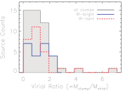
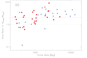
The virial ratio ($=M_{clump}/M_{virial}$) versus the clump mass is shown in Fig. 9(c). The green dotted horizontal line marks the line of gravitational instability (i.e. $M_{clump}=M_{virial}$). Clumps below this line are unbound and will not collapse under gravity. There are 87 per cent (40 of 46) of the clumps with masses larger than the virial mass, suggesting that they will form stars or are already undergoing star formation. The IR-bright and IR-faint clumps have a mean virial ratio of 2.7 and 2.8, respectively, and a median virial ratio of 2.8 and 2.1, respectively. However, magnetic fields can prevent the collapse of a clump and by assuming the equipartition of kinetic and magnetic energy, the relationship between clump and virial masses can be found to be $M_{clump}=2M_{virial}$ (e.g. Bertoldi & McKee 1992) and is shown by the dashed green horizontal line. By including magnetic fields, the number of clumps which are gravitationally unstable becomes 70 per cent (14 of 20) and 54 per cent (14 of 26), for IR-bright and IR-faint clumps, respectively.

Figure 9: Correlations between physical parameters. IR-bright clumps are represented by blue filled triangles. IR-faint clumps are represented by red filled squares. The excluded IR-bright and IR-faint clumps are represented by blue hollow triangles and red hollow squares, respectively. For (b): The blue dotted line displays the fit to the IR-bright clumps. The red dashed line displays the fits to the IR-faint clumps. The black dashed dot line displays the fit to both samples. These fits do not include the clumps that have been excluded, as per §4.1.1. The black solid line displays the 1:1 line. For (c): The green dotted line displays the equilibrium between clump and virial masses, while the green dashed line shows the equilibrium between kinetic and magnetic energy.

4.5 Kolmogorov–Smirnov test

The Kolmogorov–Smirnov (K-S) test is used to test whether our IR-bright and IR-faint clumps are likely to be drawn from the same population. We perform a K-S test on the physical parameters derived from the NH3 (1,1) and (2,2) spectra. To compare the cumulative distribution functions of the physical parameters for the IR-bright and IR-faint clumps, $S_{\mathrm{IR-bright}}(x)$ and $S_{\mathrm{IR-faint}}(x)$, the K-S statistic, can be written following Press et al. (1992, chap. 14) as:

$$\mathrm{D}=\max_{-\infty<x<\infty}|S_{\mathrm{IR-bright}}(x)-S_{\mathrm{IR-faint}}(x)|$$ (11)

To calculate the significance of the KS test:

$$\mathrm{Q}_{KS}(\lambda)=2\sum_{j=1}^{\infty}(-1)^{j-1}\mathrm{e}^{-2j^{2}\lambda^{2}}$$ (12)

where

$$\lambda=\left[{\sqrt{N_{eff}}+\dfrac{0.11}{\sqrt{N_{eff}}}}\right]D$$ (13)

and $N_{eff}$ is the effective number of data points, with

$$N_{eff}=\dfrac{N_{1}N_{2}}{N_{1}+N_{2}}$$ (14)

where $N_{1}$ and $N_{2}$ are the two distributions to be tested.

The significance and K-S statistic for the clump and derived parameters can be seen in Table 6. The significances were calculated to be 0.0078, 0.3747, 0.0162, 0.0002, 0.0446 and 0.0056 for peak flux, clump radius, NH3 (1,1) FWHM, kinetic temperature, clump mass, and virial mass, respectively. We note that the significance of the cumulative distribution functions between the two populations for the kinetic temperature are over the 0.003 significance level (3$\sigma$) than if they were drawn from the same population (Wall & Jenkins, 2012). Through accurate kinetic temperatures, we confirm that 8 ${\rm\mu m}$ emission traces the warm dust and gas. In Fig. 3, the NH3 (1,1) FWHM displays a difference between the two populations, however the significance in the K-S test is below the 3$\sigma$ level. The same outcome is not apparent through the clump radius or either the clump or virial masses. The effect of turbulence is important to high-mass star formation as it can encourage the development of stars above the mass threshold. However, if the amount of turbulence is too high, it can discourage star formation (Padoan, 1995). As the NH3 (1,1) linewidths (1.1–4.5 km s^-1) are larger than the thermal component ($\sim$0.28 km s^-1 for $T_{\rm{kin}}$=30 K), all our clumps show varying amounts of turbulence. However, the K-S test was unable to find a significant difference between the IR-bright and IR-faint clumps, so we are unable to find a link between the amount of turbulence and 8 ${\rm\mu m}$ emission. The K-S test was unable to distinguish a significant difference for the clump radius. This is important because a significant difference would indicate that different algorithms and input settings would drastically affect the parameters derived from the clumps.

Table 6: Results from the Kolmogorov–Smirnov (K-S) test of IR-bright and IR-faint clumps. Column 2 shows the significance (Q_KS) of the K-S test and Column 3 shows the maximum deviation (D) between the cumulative distribution function of the IR-bright and IR-faint clumps.

Clumps with detectable NH3 (1,1) and (2,2)
Parameter	QKS	D
Peak flux	0.0059	0.42
Clump radius	0.4694	0.21
Total flux	0.0436	0.34
NH3 (1,1) FWHM	0.0136	0.43
Column density	0.1917	0.30
Kinetic temperature	0.0002	0.59
Clump mass	0.0595	0.35
Virial mass	0.0041	0.48
Clumps in the main cloud†
Parameter	QKS	D
Peak flux	0.0078	0.42
Clump radius	0.3742	0.23
Total flux	0.0297	0.36
NH3 (1,1) FWHM	0.0162	0.44
Column density	0.3667	0.26
Kinetic temperature	0.0002	0.61
Clump mass	0.0446	0.39
Virial mass	0.0056	0.48

$\dagger$The clumps designated as “main cloud” are those with calculated parameters from the NH3 spectra but exclude those as per §4.1.1.

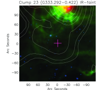
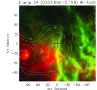
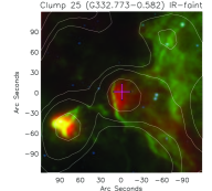
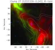
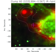
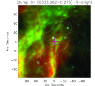
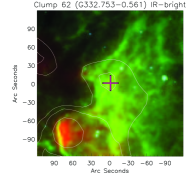
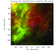
4.6 Environments around interesting sources

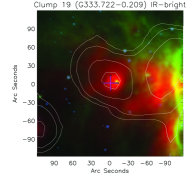
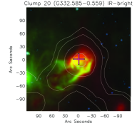
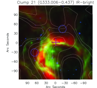
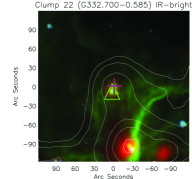
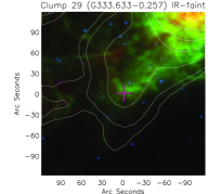
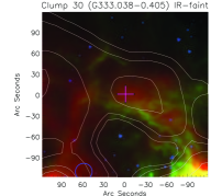
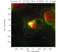
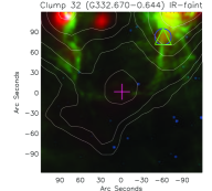
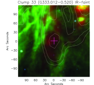
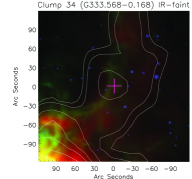
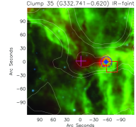
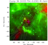
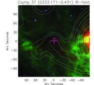
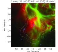
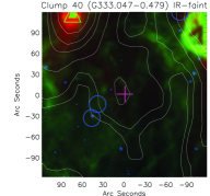
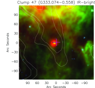
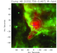
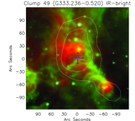
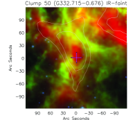
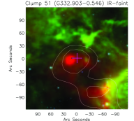
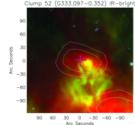
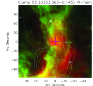
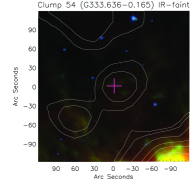
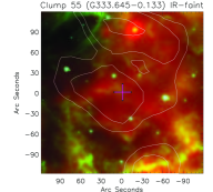
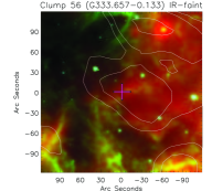
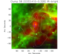
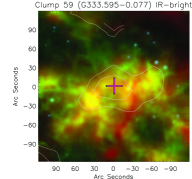
Here we discuss sources that deserve further detail than those provided by Columns 8, 9 and 10 of Table 1. Infrared composite images centered on the peak emission of the dust clumps identified by clumpfind can be found in Fig. A. NH3 (1,1) and (2,2) emission detected towards the peak emission of each clump can be found in Fig. B.

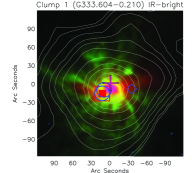
Clump 1 (G333.604$-$0.210). This is the brightest IR source in the southern Galactic Plane (Becklin et al., 1973). Fujiyoshi et al. (2005, 2006) found that this Hii region is excited by a cluster of O and B stars. Fujiyoshi et al. (2006) also found a complex H90$\alpha$ radio recombination line spectrum which they suggest may be caused by champagne outflows. NH3 emission is weak and shows absorption but both (1,1) and (2,2) show similar intensities.

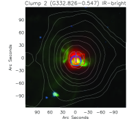
Clump 2 (G332.826$-$0.547) and Clump 60 (G332.894$-$0.567). These clumps appear to be related to a 8 ${\rm\mu m}$ bubble. Clump 2 (G332.894$-$0.567) coincides with an Hii region and YSO (Urquhart et al., 2008) which is within the extent of RCW 106 (Rodgers et al., 1960). There are H2O, Class II CH3OH and OH masers. There is bifurcated 8 ${\rm\mu m}$ emission which may explain the broad NH3 (1,1) and (2,2) spectrum. The NH3 (1,1) spectrum appears to be blended with no clear baseline between the hyperfine transitions. The Hii region and YSO also coincides with a 160 ${\rm\mu m}$ diffuse source. Clump 60 (G332.894$-$0.567) is not associated with any known maser activity and there is no detectable NH3 emission.

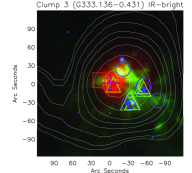
Clump 3 (G333.136$-$0.431). This clump contains an assortment of masers however the peak of the SIMBA dust clump coincides with a 160 ${\rm\mu m}$ diffuse source as well as OH and 6.7 GHz Class I CH3OH masers. The peak of this SIMBA dust clump is surrounded by 8 ${\rm\mu m}$ emission with an assortment of maser activity. There are four clusters of maser activity around the peak with two clusters containing 6.7 GHz Class I CH3OH and H2O masers as well as 44.07 and 95.1 GHz class II CH3OH masers. It is rare to see the two classes of CH3OH masers in the same cluster. Class II CH3OH masers are closely associated with YSOs, while Class I CH3OH masers are associated with shocks and cloud-cloud collisions. There may be triggered star formation occurring in this 8 ${\rm\mu m}$ arc which has allowed for the two classes of masers to be seen at the same time. A collision between clouds would create the Class I CH3OH masers but also trigger star formation which leads to outflows, YSOs and the Class II CH3OH masers.

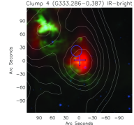
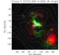
Clump 4 (G333.286$-$0.387) and Clump 5 (G333.309$-$0.369). These clumps appear to be local peaks in a larger clump. Clump 4 contains multiple point sources with a water maser and was classified by the RMS survey as a Hii region. Clump 5 was classified by the RMS survey as a diffuse Hii region.

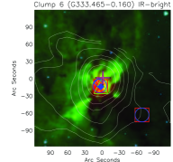
Clump 6 (G333.465$-$0.160). This clump contains a mixture of Class I and II CH3OH masers as well as a water maser. It has a lot of 8 ${\rm\mu m}$ emission around a diffuse 160 ${\rm\mu m}$ source. This looks like Clump 2 (G332.826$-$0.547) but with significantly more 8 ${\rm\mu m}$ emission. This may be a later evolutionary stage but the NH3 (1,1) and (2,2) do not show blended spectra, which could indicate turbulence, like Clump 2 (G332.826$-$0.547).

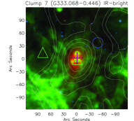
Clump 7 (G333.068$-$0.446). Satellite lines can be seen in both the NH3 (1,1) and (2,2). There are Class II CH3OH masers associated with the SIMBA dust peak and a Class II CH3OH and water maser offset by $\sim$1 arcmin on either side of the SIMBA dust peak.

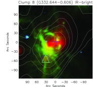
Clump 8 (G332.644$-$0.606), Clump 10 (G332.691$-$0.612), Clump 12 (G332.676$-$0.615) and Clump 22 (G332.700$-$0.585). There are two 160 ${\rm\mu m}$ sources within 8 ${\rm\mu m}$ arcs on either side of another 160 ${\rm\mu m}$ source. There is a 6.7 GHz Class I CH3OH and water maser along the west 8 ${\rm\mu m}$ arc, however neither is coincident with the SIMBA dust peak. The ionising source of this bubble is unknown; however, further analysis is required to show if it is expanding outwards from Clump 12 (G332.676$-$0.615). These clumps are also within the region classified by Rodgers et al. (1960) as RCW 106.

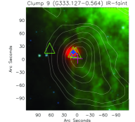
Clump 9 (G333.127$-$0.564). This is a relatively isolated, cold dust clump which coincides with the second brightest SiO source within this GMC (Lo et al., 2007). There are low levels of the NH3 (2,2) satellite lines.

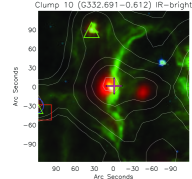
Clump 10 (G332.691$-$0.612). This is an elongated Hii region and could be star formation triggered by a bow shock of a nearby protostellar object. This clump could be associated with nearby Clump 12 (G332.676$-$0.615). The maser at the top corresponds to a YSO and Hii region.

Clump 11 (G333.018$-$0.449) and Clump 21 (G333.006$-$0.437). These two clumps are on the edge of the same 8 ${\rm\mu m}$ arc. The SIMBA dust clumps appear to coincide with 160 ${\rm\mu m}$ emission. Both clumps have H2O masers on the far side of the 8 ${\rm\mu m}$ arc. Both clumps have high $T_{\rm{kin}}$. Clump 11 (G333.018$-$0.449) has a $T_{\rm{kin}}$ of 35.6 K and Clump 21 (G333.006$-$0.437) has a $T_{\rm{kin}}$ of 63.6 K.

Clump 13 (G333.524$-$0.272), Clump 27 (G333.539$-$0.245) and Clump 46 (G333.521$-$0.239). Clump 13 (G333.524$-$0.272) appears to follow the 160 ${\rm\mu m}$ emission which appears to be compressed between two 8 ${\rm\mu m}$ arcs. There is no known maser emission in this region. Clump 27 (G333.539$-$0.245) also appear to follow the compressed 160 ${\rm\mu m}$ emission however the intensity is lower. Clump 46 (G333.521$-$0.239) is also associated but the 160 ${\rm\mu m}$ emission is the weakest of the three.

Clump 14 (G332.985$-$0.487), Clump 18 (G333.074$-$0.558), Clump 19 (G333.722$-$0.209), Clump 39 (G333.642$-$0.106), Clump 47 (G333.074$-$0.399), Clump 51 (G332.903$-$0.546) and Clump 58 (G333.410$-$0.328). These clumps contain a compact 160 ${\rm\mu m}$ object towards the position of the peak SIMBA position. There is no 4.5 or 8 ${\rm\mu m}$ emission nearby. It is likely to be the earliest stage of star formation.

From the environment around select clumps, there are a variety of star formation stages within the G333 GMC. This ranges from isolated, compact 160 ${\rm\mu m}$ objects, to areas with complex infrared emission and multiple masers. There also appears to be possible triggered star formation [e.g. Clump 3 (G333.136$-$0.431)]. In future papers, we will be combining the molecular and dust information for all 63 clumps identified in this paper, to characterise the clumps in relation to the evolution of star formation within the G333 GMC.

5 Summary and Conclusions

In this paper we have presented data from the two lowest inversion transitions of NH3 in the G333 giant molecular cloud with the 70-m Tidbinbilla radio telescope. Our main conclusions are as follows:

(1) There were 63 SIMBA 1.2-mm dust clumps identified with clumpfind and pointed NH3 observations were conducted towards the peak of each clump. The peak of each clump was offset from the clump centroid by between 1.6 and 39.5 arcsec.

(2) A variety of environments were identified within the G333 GMC and the sample was separated into 30 IR-bright and 33 IR-faint clumps. One clump from each category was identified via NH3 (2,2) emission, to not be associated with the $v_{\rm{LSR}}$ of the G333 GMC, and one clump was identified to have an inaccurate $T_{\rm{kin}}$; resulting in 29 IR-bright and 31 IR-faint clumps. The NH3 (1,1) and (2,2) were fitted for 20 IR-bright and 26 IR-faint clumps, with mean $T_{\rm{kin}}$ values of 24.2 K and 19.3 K, respectively.

(3) We found that the clumps appeared to cluster into three regions. The IR-bright clumps were found predominately towards the centre of each region, especially for Regions B and C. This may indicate sequentially triggered star formation in the vicinity around IR-faint clumps.

(4) Using NH3 (1,1) and (2,2), the clump masses were found to be between 278 and 13036 M_⊙. The dust temperature is often assumed: 20 K for isolated clumps and 40 K for Hii regions; however this assumption can significantly shift the masses of the clumps (e.g. for 20 K the masses of our clumps were 251–23723 M_⊙, and for 40 K the masses of our clumps were 105–9951 M_⊙) and can affect whether the clump is determined to be bound and will collapse onto itself, or if it is unbound and remains a starless core. Hence accurate measurements of kinetic temperatures are needed for studies of the gravitationally bound state of clumps.

(5) The largest clumps are also the most unstable. We find that the clumps with signs of star formation are predominately associated with the least stable clumps. This may be due to feedback from an internal heating source. We found that 70 per cent of the clumps had masses larger than the virial mass (187–6848 M_⊙), suggesting that they will form stars or are already undergoing star formation.

(6) A K-S test showed that the $T_{\rm{kin}}$ for IR-bright and IR-faint clumps have a much smaller probability of being drawn from the same population. A tentative difference between the two populations in terms of FWHM could indicate a contribution due to feedback. No difference was seen for the other physical parameters. We conclude that IR-bright and IR-faint clumps can have the same masses but that the warmer regions are more evolved.

This is the fourth paper in a series of papers utilising molecular line observations of the G333 giant molecular cloud associated with RCW 106 (G333 GMC). In this paper we reported on the selection of dense clumps based on SIMBA dust emission and pointed NH3 (1,1) and (2,2) observations towards these clumps. Future papers in the series will analyse the individual clumps and combine the information presented in this paper with the molecular 3-mm tracers presented in Bains et al. (2006), Wong et al. (2008) and Lo et al. (2009), and dust from the Spitzer Space Telescope and the Herschel Space Observatory.

SUPPORTING INFORMATION

Additional Supporting Information may be found in the online version of this article.

Figure A. Infrared composite images centred on the peak of the 63 SIMBA dust clumps.
Figure B. NH3 (1,1)  and (2,2) spectra towards the peak of the 63 SIMBA dust clumps.

Figure A: Infrared composite images centered on the peak dust emission of each clump identified with clumpfind. Spitzer 4.5 (shocked gas) and 8.0 ${\rm\mu m}$ (PAH⁺ emission), and Herschel 160 ${\rm\mu m}$ (cool dust) are shown in blue, green and red, respectively. The SIMBA dust contours have been set to 0.1, 0.2, 0.5, 1, 1.5, 2.5, 5, 10, 15, 25 and 35 mJy beam^-1. H2O  masers are identified by blue circles. Class I CH3OH  masers are identified by unfilled (44.07 GHz) and filled (95.1 GHz) blue diamonds. Class II CH3OH  masers are identified by unfilled (6.7 GHz) and filled (12.2 GHz) green triangles. OH masers are identified by unfilled (1665/1667/1720 MHz) and filled (6.035 GHz) red squares.

Figure A: continued

Figure A: continued

Figure A: continued

Figure A: continued

Figure A: continued

Figure B: NH3 emission detected towards the peak dust emission of each clump identified with clumpfind. The NH3 (1,1) and (2,2) spectra are in the top and bottom panel, respectively. The model fits to these data are shown in green. Clumps 1-6 are shown l-r, t-b.

Figure B: continued

Clumps 7-12 are shown l-r, t-b.

Figure B: continued

Clumps 13-18 are shown l-r, t-b.

Figure B: continued

Clumps 19-24 are shown l-r, t-b.

Figure B: continued

Clumps 25-30 are shown l-r, t-b.

Figure B: continued

Clumps 31-36 are shown l-r, t-b.

Figure B: continued

Clumps 37-42 are shown l-r, t-b.

Figure B: continued

Clumps 43-48 are shown l-r, t-b.

Figure B: continued

Clumps 49-54 are shown l-r, t-b.

Figure B: continued

Clumps 55-60 are shown l-r, t-b.

Figure B: continued

Clumps 61-63 are shown l-r, t-b.

References

- Bains et al. (2006) Bains I., Wong T., Cunningham M., Sparks P., Brisbin D., Calisse P., Dempsey J. T., Deragopian G., et al., 2006, MNRAS, 367, 1609
- Becklin et al. (1973) Becklin E. E., Frogel J. A., Neugebauer G., Persson S. E., Wynn-Williams C. G., 1973, ApJ, 182, L125
- Benjamin et al. (2003) Benjamin R. A., et al., 2003, PASP, 115, 953
- Bertoldi & McKee (1992) Bertoldi F., McKee C. F., 1992, ApJ, 395, 140
- Braz & Scalise (1982) Braz M. A., Scalise E., Jr., 1982, A&A, 107, 272
- Breen et al. (2007) Breen S. L., et al., 2007, MNRAS, 377, 491
- Breen et al. (2010) Breen S. L., Caswell J. L., Ellingsen S. P., Phillips C. J., 2010, MNRAS, 406, 1487
- Breen et al. (2012) Breen S. L., Ellingsen S. P., Caswell J. L., Green J. A., Voronkov M. A., Fuller G. A., Quinn L. J., Avison A., 2012, MNRAS, 421, 1703
- Breen et al. (2013) Breen S. L., Ellingsen S. P., Contreras Y., Green J. A., Caswell J. L., Stevens J. B., Dawson J. R., Voronkov M. A., 2013, MNRAS, 435, 524
- Carey et al. (2009) Carey S. J., et al., 2009, PASP, 121, 76
- Caswell et al. (2011) Caswell J. L., et al., 2011, MNRAS, 417, 1964
- Caswell, Haynes, & Goss (1980) Caswell J. L., Haynes R. F., Goss W. M., 1980, AuJPh, 33, 639
- Caswell, Vaile, & Forster (1995) Caswell J. L., Vaile R. A., Forster J. R., 1995, MNRAS, 277, 210
- Caswell (1996) Caswell J. L., 1996, MNRAS, 279, 79
- Caswell (1997) Caswell J. L., 1997, MNRAS, 289, 203
- Caswell (1998) Caswell J. L., 1998, MNRAS, 297, 215
- Caswell (2009) Caswell J. L., 2009, PASA, 26, 454
- Churchwell et al. (2009) Churchwell E., et al., 2009, PASP, 121, 213
- Cyganowski et al. (2008) Cyganowski C. J., et al., 2008, AJ, 136, 2391
- Danby et al. (1988) Danby G., Flower D. R., Valiron P., Schilke P., Walmsley C. M., 1988, MNRAS, 235, 229
- Dunham et al. (2011) Dunham M. K., Rosolowsky E., Evans N. J., II, Cyganowski C., Urquhart J. S., 2011, ApJ, 741, 110
- Ellingsen et al. (1996) Ellingsen S. P., von Bibra M. L., McCulloch P. M., Norris R. P., Deshpande A. A., Phillips C. J., 1996, MNRAS, 280, 378
- Ellingsen (2005) Ellingsen S. P., 2005, MNRAS, 359, 1498
- Garay et al. (2004) Garay G., Faúndez S., Mardones D., Bronfman L., ChiniR., Nyman L.-Å., 2004, ApJ, 610, 313
- Fujiyoshi et al. (2005) Fujiyoshi T., Smith C. H., Moore T. J. T., Lumsden S. L., Aitken D. K., Roche P. F., 2005, MNRAS, 356, 801
- Fujiyoshi et al. (2006) Fujiyoshi T., Smith C. H., Caswell J. L., Moore T. J. T., Lumsden S. L., Aitken D. K., Roche P. F., 2006, MNRAS, 368, 1843
- Goss & Shaver (1970) Goss W. M., Shaver P. A., 1970, AuJPA, 14, 1
- Griffin et al. (2010) Griffin M. J., et al., 2010, A&A, 518, L3
- Hildebrand (1983) Hildebrand R. H., 1983, QJRAS, 24, 267
- Hill et al. (2010) Hill T., Longmore S. N., Pinte C., Cunningham M. R., Burton M. G., Minier V., 2010, MNRAS, 402, 2682
- Ho & Townes (1983) Ho P. T. P., Townes C. H., 1983, ARA&A, 21, 239
- Johnstone et al. (2010) Johnstone D., Rosolowsky E., Tafalla M., Kirk H., 2010, ApJ, 711, 655
- Ladd et al. (2005) Ladd N., Purcell C., Wong T., Robertson S., 2005, Publications of the Astronomical Society of Australia, 22, 62
- Li, Goldsmith, & Menten (2003) Li D., Goldsmith P. F., Menten K., 2003, ApJ, 587, 262
- Lo et al. (2007) Lo N., Cunningham M., Bains I., Burton M. G., Garay G., 2007, MNRAS, 381, L30
- Lo et al. (2009) Lo N., Cunningham M. R., Jones P. A., Bains I., Burton M. G., Wong T., Muller E., Kramer C., et al., 2009, MNRAS, 395, 1021
- Lo et al. (2011) Lo N., Redman M. P., Jones P. A., Cunningham M. R., Chhetri R., Bains I., Burton M. G., 2011, MNRAS, 415, 525
- Lockman (1979) Lockman F. J., 1979, ApJ, 232, 761
- Lumsden et al. (2013) Lumsden S. L., Hoare M. G., Urquhart J. S., Oudmaijer R. D., Davies B., Mottram J. C., Cooper H. D. B., Moore T. J. T., 2013, ApJS, 208, 11
- Luna et al. (2006) Luna A., Bronfman L., Carrasco L., May J., 2006, ApJ, 641, 938
- Manchester (1969) Manchester B. A., 1969, AuJPA, 12, 3
- Mangum et al. (1992) Mangum J. G., Wootten A., Mundy L. G., 1992, ApJ, 388, 467
- Minier et al. (2003) Minier V., Ellingsen S. P., Norris R. P., Booth R. S., 2003, A&A, 403, 1095
- Molinari et al. (2010) Molinari S., et al., 2010, PASP, 122, 314
- Mookerjea et al. (2004) Mookerjea B., Kramer C., Nielbock M., Nyman L.-Å., 2004, A&A, 426, 119
- Ott (2010) Ott S., 2010, ASPC, 434, 139
- Ossenkopf & Henning (1994) Ossenkopf V., Henning T., 1994, A&A, 291, 943
- Padoan (1995) Padoan P., 1995, MNRAS, 277, 377
- Pilbratt et al. (2010) Pilbratt G. L., et al., 2010, A&A, 518, L1
- Poglitsch et al. (2010) Poglitsch A., et al., 2010, A&A, 518, L2
- Press et al. (1992) Press, W. H., et al., 1992, Numerical Recipes in C: The Art of Scientific Computing. Cambridge University Press, New York.
- Protheroe et al. (2008) Protheroe R. J., Ott J., Ekers R. D., Jones D. I., Crocker R. M., 2008, MNRAS, 390, 683
- Rodgers et al. (1960) Rodgers A. W., Campbell C. T., Whiteoak J. B., 1960, MNRAS, 121, 103
- Roussel (2013) Roussel H., 2013, PASP, 125, 1126
- Slysh et al. (1994) Slysh V. I., Kalenskii S. V., Valtts I. E., Otrupcek R., 1994, MNRAS, 268, 464
- Spitzer Science (2009) Spitzer Science C., 2009, yCat, 2293, 0
- Swift et al. (2005) Swift J. J., Welch W. J., Di Francesco J., 2005, ApJ, 620, 823
- Tafalla et al. (2004) Tafalla M., Myers P. C., Caselli P., Walmsley C. M., 2004, A&A, 416, 191
- Urquhart et al. (2008) Urquhart J. S., Hoare M. G., Lumsden S. L., Oudmaijer R. D., Moore T. J. T., 2008, ASPC, 387, 381
- Urquhart et al. (2011) Urquhart J. S., et al., 2011, MNRAS, 418, 1689
- Urquhart et al. (2014) Urquhart J. S., Figura C. C., Moore T. J. T., Hoare M. G., Lumsden S. L., Mottram J. C., Thompson M. A., Oudmaijer R. D., 2014, MNRAS, 437, 1791
- Vallée (2008) Vallée J. P., 2008, AJ, 135, 1301
- Voronkov et al. (2014) Voronkov M. A., Caswell J. L., Ellingsen S. P., Green J. A., Breen S. L., 2014, MNRAS, 334
- Wall & Jenkins (2012) Wall J. V., Jenkins C. R., 2012, psa..book,
- Walsh et al. (2011) Walsh A. J., et al., 2011, MNRAS, 416, 1764
- Walmsley & Ungerechts (1983) Walmsley C. M., Ungerechts H., 1983, A&A, 122, 164
- Walsh et al. (1998) Walsh A. J., Burton M. G., Hyland A. R., Robinson G., 1998, MNRAS, 301, 640
- Wienen et al. (2012) Wienen M., Wyrowski F., Schuller F., Menten K. M., Walmsley C. M., Bronfman L., Motte F., 2012, A&A, 544, A146
- Williams, de Geus, & Blitz (1994) Williams J. P., de Geus E. J., Blitz L., 1994, ApJ, 428, 693
- Wong et al. (2008) Wong T., Ladd E. F., Brisbin D., Burton M. G., Bains I., Cunningham M. R., Lo N., Jones P. A., et al., 2008, MNRAS, 386, 1069
- Zinnecker & Yorke (2007) Zinnecker H., Yorke H. W., 2007, ARA&A, 45, 481