Stability of the accretion of a ghost condensate onto the Schwarzschild black hole

Abstract

We study the linear stability of a nongravitating, steady-state, spherically symmetric ghost condensate accreting onto a Schwarzschild black hole using two methods. The first one is based on the conservation of the energy-momentum tensor of the perturbations (whose propagation is determined by the effective metric), and involves determination of the sign of the time derivative of the energy of the perturbations. The second method employs the positivity of the effective potential. Both methods yield the result that the system is stable, but the second one is less practical, since it involves lengthier calculations and requires the explicit form of the background solution for the scalar field.

I Introduction

Black hole solutions of General Relativity in four dimensions have been shown to be dynamically stable at the linear level by perturbing the corresponding equations of motion. In the case of Schwarszchild’s solution, the stability was originally studied by Regge and Wheeler (Regge1957, ), while the stability of the Reissner-Nordstrom geometry was determined in (Moncrief1974a, ; Moncrief1974b, ). Kerr’s solution was shown to be stable in (Whiting1989, ). Due to the fact that black holes are often surrounded by matter, it is important to study also the stability of solutions in which there is matter accreting onto the black hole, as well as onto compact objects in general. The hypothesis of spherically symmetric accretion is frequently adopted as a first step in the building of more realistic models. In this vein, the accretion of a barotropic fluid with this symmetry onto a star was studied in the newtonian regime by (Bondi1952, ), and its stability proved in several papers (see for instance (Garlick1979, ) and (Petterson1980, ), and the references cited in (Mandal2007, )). The equations of motion for a steady-state spherical symmetric flow onto a relativistic compact object were set and solved in (Michel1972, ). The stationary, spherically symmetric, polytropic and inviscid accretion flow onto a Schwarzschild black hole was studied with techniques from dyamical systems in (Mandal2007, ) . The perturbations of a non-self gravitating perfect fluid in potential flow and stationary, spherical accretion onto a Schwarzschild black hole were shown to be stable at the linear level by Moncrief (Moncrief1980, ), using the fact that their evolution is governed by what he called the sonic metric (and is now known to be a specific instance of the effective metric, see for instance (Barcelo2005, )).

We shall study here the linear stability of the accretion of a scalar field with a non-canonical kinetic term onto a Schwarzschild black hole. These scalar field models, generically called $k$-essence, have been widely used to describe the accelerated expansion of the universe according to the standard cosmological model (Armendariz2000, ; Armendariz2000b, ; Tsujikawa2010, ), and also to give a unified model for dark matter and dark energy (Scherrer2004, ). Cosmological perturbations in the so-called $k$-inflation have been analyzed in (Garriga1999, ). In (Akhoury2011b, ), the gravitational collapse of a Born-Infeld-like $k$-essence model was investigated. The collapse with other Lagrangians was studied using Painlevè-Gullstrand coordinates in (Leonard2011, ). Regarding black holes, their existence with a non-canonical scalar field as a matter source was studied in (Graham2014, ). The steady-state accretion of a $k$-essence field onto a Reissner-Nordstrom black hole was studied in (Babichev2008, ). It was proved in (Akhoury2008, ) that the existence of stationary configurations of a non-canonical scalar field requires that the Lagrangian be invariant with respect to the field redefinition $\phi\rightarrow\phi+c$, for all values of the constant $c$. The steady-state spherically symmetric accretion of a ghost condensate in the gravitational field of a Schwarzschild black hole was studied analytically in (Frolov2004, ). Numerical simulations of the accretion onto a Schwarzschild black hole of test scalar fields with a Dirac-Born-Infeld type Lagrangian, and for the ghost condensate of (Frolov2004, ) were analyzed in (Akhoury2011a, ).

The main goal of this paper is to study the stability of the stationary accretion presented in (Frolov2004, ) with the method developed in (Moncrief1980, ) . We shall begin in Sect.II with a short review of the effective metric in the case of a nonlinear field theory for a scalar field, including the method developed by Moncrief adapted to the case at hand. In Sect.III the specific model of a nonlinear scalar field accreting onto a black hole presented in (Frolov2004, ) will be reviewed, and shown to be stable. In Section V we shall obtain the same result (though with a lot more effort from the point of view of calculations) using the more traditional method of the effective potential. We close with a discussion in Sect.VI.

II Effective metric

The propagation of the excitations of any nonlinear field theory on a fixed background is governed by an effective metric that depends on the background field configuration and on the details of the nonlinear dynamics obeyed by the field (see (Barcelo2005, ) for a complete review). The case of a nonlinear scalar field has been studied in (Barcelo2001, ), and it was shown in (Goulart2011, ) that the effective metric can be classified in different types according to whether the gradient of the scalar field is timelike, null, or spacelike. Let us briefly review how the effective metric arises in theories in which the action is given by

$$S[\phi]=\int\sqrt{-g}\;\mathcal{L}(W)\;d^{4}x,$$ (1)

where $W\equiv g^{\mu\nu}\nabla_{\mu}\phi\nabla_{\nu}\phi$ and $g_{\mu\nu}$ is the background metric. The corresponding EOM is

$$\left[\sqrt{-g}\;(\mathcal{L}_{W}g^{\mu\nu}+2\mathcal{L}_{WW}\Phi^{\mu\nu})\;\right]\nabla_{\mu}\nabla_{\nu}\phi=0,$$ (2)

where ${\cal L}_{W}\equiv\frac{\partial{\cal L}}{\partial W}$, etc, and $\Phi^{\mu\nu}\equiv g^{\mu\alpha}\phi_{\alpha}g^{\nu\beta}\phi_{\beta}.$ By perturbing the EOM with

$$\phi=\phi_{0}+\varepsilon\phi_{1},$$ (3)

where $\phi_{0}$ is the backgound field (solution of Eqn.(2) for a given Lagrangian), $\phi_{1}$ is the perturbation, and $\varepsilon$ a parameter for power counting, we get for the EOM of the perturbations (see details in Barcelo2001 ; Goulart2011 )

$$\left[\sqrt{-g}\right.(\mathcal{L}_{W}g^{\mu\nu}+2\mathcal{L}_{WW}\Phi^{\mu\nu})\left|{}_{0}\;\phi_{1,\mu}\right],_{\nu}=0,$$ (4)

where all the quantities in the parentheses are evaluated at the background. Defining $\widetilde{g}^{\mu\nu}$ by

$$\sqrt{-\widetilde{g}}\text{ }\widetilde{g}^{\mu\nu}=\sqrt{-g}\left.\left(\mathcal{L}_{W}g^{\mu\nu}+2\mathcal{L}_{WW}\Phi^{\mu\nu}\right)\right|_{0},$$ (5)

Eqn.(4) can be written as

$$(\sqrt{-\widetilde{g}}\text{ }\widetilde{g}^{\mu\nu}\phi_{1,\mu}),_{\nu}=0.$$ (6)

It follows from Eqn.(5) that

$$\widetilde{g}^{\mu\nu}=\frac{M^{\mu\nu}}{\sqrt{-g}\sqrt{M}},$$ (7)

where $M^{\mu\nu}\equiv\left.\mathcal{L}_{W}g^{\mu\nu}+2\mathcal{L}_{WW}\Phi^{\mu\nu}\right|_{0}$. Different aspects of the effective geometry for scalar fields with noncanonical Lagrangians, described by $\widetilde{g}_{\mu\nu}$, i.e. the inverse of the tensor defined in Eqn.(5), were studied in (Babichev2006, ; Babichev2007, ; Goulart2011, ). Among them, we would like to point out here that the effective metric inherits the symmetries of the background metric. This can be seen as follows. If $X$ be a Killing vector of the backgroud metric, then $\pounds_{X}g_{\mu\nu}=0$. Since $\pounds_{X}\phi_{0}=0$, the effective metric satisfies $\pounds_{X}\widetilde{g}_{\mu\nu}=0$.

By perturbing the action given in Eqn.(1), it follows that the action for the perturbations (corresponding to the $O(\varepsilon^{2})$ term) reads

$$S_{2}=\int\sqrt{-\widetilde{g}}\text{ }\widetilde{g}^{\mu\nu}\phi_{1,\mu}\phi_{1,\nu}d^{4}x.$$ (8)

The variation of this action w.r.t. $\widetilde{g}^{\mu\nu}$ yields the energy-momentum tensor of the perturbations, given by

$$\widetilde{T}_{\nu}^{\mu}=\widetilde{g}^{\mu\lambda}\phi_{1,\lambda}\phi_{1,\nu}-\frac{1}{2}\delta_{\nu}^{\mu}\widetilde{g}^{\alpha\beta}\phi_{1,\alpha}\phi_{1,\beta},$$ (9)

which satisfies $\widetilde{\nabla}_{\mu}\widetilde{T}^{\mu}_{\nu}=0$, where $\widetilde{\nabla}_{\mu}$ is the covariant derivative defined with the efective metric.

As discussed in (Moncrief1980, ), if $X$ is a Killing vector of the effective metric it follows that

$$\widetilde{\nabla}_{\mu}\left(X^{\nu}\widetilde{T}_{\nu}^{\mu}\right)=0,$$ (10)

which can be rewritten as

$$\partial_{\nu}\left(\sqrt{-\widetilde{g}}{X}^{\mu}\widetilde{T}_{\mu}^{\nu}\right)=0.$$ (11)

Choosing ${X}^{\nu}=\delta_{t}^{\nu}$ and integrating Eqn.(11) in a 3-volume $V$,

$$\int_{V}\partial_{t}(\sqrt{-\tilde{g}}\widetilde{T}_{t}^{t})d^{3}x+\int_{V}\partial_{i}(\sqrt{-\tilde{g}}\widetilde{T}_{t}^{i})d^{3}x=0.$$ (12)

Defining the energy of the perturbations by $\widetilde{E}=\int_{V}\sqrt{-\widetilde{g}}$ $\widetilde{T}_{t}^{t}d^{3}x$, and using Gauss theorem, Eqn.(12) can be written as

$$\frac{d\widetilde{E}}{dt}=-\int_{\Sigma}d\Sigma_{i}\sqrt{-\widetilde{g}}\text{ }\widetilde{T}_{t}^{i}.$$ (13)

This is the key result obtained by Moncrief in (Moncrief1980, ). By a proper choice of the surface $\Sigma$ enclosing the volume $V$, and using the properties of the fields on $\Sigma$, it is possible to determine the sign of the integral without solving it, thus determining if the system is linearly stable. We shall use this method to determine if the model presented in the next section is stable.

III Accretion of a nonlinear scalar field onto a Schwarzschild black hole

The model studied in (Frolov2004, ) (called “ghost condensation”) was proposed in (ArkaniHamed2003, ), and consists of a nongravitating nonlinear scalar field with Lagrangian

$$\mathcal{L}(W)=\frac{1}{2}(W-A)^{2},$$ (14)

(where $A$ is a constant to be determined later) in the background of a Schwarzschild black hole,

$$ds^{2}=fdt^{2}-f^{-1}dr^{2}-r^{2}d\Omega^{2},$$ (15)

with

$$f(r)=\left(1-\frac{2M}{r}\right).$$ (16)

From the assumption of a stationary background and spherical symmetry, it follows that

$$\phi_{0}(t,r)=t+\psi_{0}\left(r\right).$$ (17)

Using Eqn.(15) in 2, the EOM for $\psi_{0}$ is

$$\partial^{*}_{r}(r^{2}{\cal L}_{W}\partial^{*}_{r}\psi_{0})=0,$$

where $\partial^{*}_{r}\equiv f(r)\partial_{r}$. This equation can be integrated to yield

$$\mathcal{L}_{W}\text{ }\partial^{*}_{r}\psi_{0}=\alpha\frac{r_{g}^{2}}{r^{2}},$$ (18)

where $\alpha$ is an integration constant, which is related to the accretion rate through $\dot{M}=2\alpha\times 4\pi r_{\rm g}^{2}M^{4}$ (Frolov2004, ).
Using the variables $v\equiv\partial^{*}_{r}\psi_{0}$ and $f$, and the Lagrangian given in Eqn.(14), this equation can be written as

$$\left(\frac{1-v^{2}}{f}-A\right)v=\alpha(1-f^{2}).$$ (19)

As shown in (Frolov2004, ), there is only one trajectory that goes from an homogeneous solution at infinity, passes through a sonic horizon (which is the 2-surface of constant $r$ such that $v_{\perp}^{2}=c_{s}^{2}$, where $c_{s}$ is the velocity of sound (Bilic1999, )), and reaches the Schwarzschild horizon $r_{\rm g}$. This trajectory is depicted in Fig. 1. It follows from the figure and the definitions of $v$ and $f$ that $\partial_{r}\psi_{0}\geq 0$, a piece of information that will be used below.

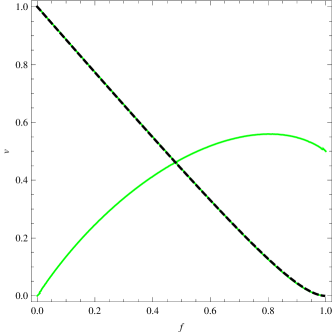
Figure 1: The figure shows in green two trajectories (for $A=3/4$) that pass through the sonic horizon $r_{\rm s}$ (located at the intersection of the curves). They correspond to $\alpha=1.51833455$. The physically relevant (and unique) trajectory for the problem at hand is the one that starts at infinity ($f=1$) with zero radial velocity and reaches Schwarzschild’s horizon ($f=0$) passing through the sonic horizon. Also shown is the plot of the analytic form for the relevant trajectory, to be used in Sect.V (dotted black curve).

IV Stability using the time variation of the energy of the perturbations

To evaluate the stability of the system reviewed in the last section using the integral given in Eqn.(13), it is convenient to choose the volume $V$ as that encompassed between the surfaces $r=r_{\rm s}$ and $r\rightarrow\infty$. Since the fields are such that

$$\sqrt{-\widetilde{g}}\;\widetilde{g}^{rr}\rightarrow\sqrt{-g}g^{rr}=r^{2}\sin\theta,\;\;\;\;\;\widetilde{g}^{rt}\rightarrow 0\;\;{\mbox{for}}\;\;r\rightarrow\infty,$$ (20)

the integral at infinity reduces to

$$I_{1}=-\int_{\Sigma_{\infty}}\left.\sqrt{-\tilde{g}}\;\phi_{1,r}\phi_{1,t}\widetilde{g}^{rr}\right|_{r\rightarrow\infty}d\Sigma_{r}.$$ (21)

The assumption of the finiteness of the energy of the perturbations, given by

$$\widetilde{E}=\int_{V}\sqrt{-\widetilde{g}}\;\widetilde{T}_{t}^{t}d^{3}x,$$

leads to the following behaviour of the perturbations at infinity:

$$\phi_{1,t}\sim\frac{a}{r^{\frac{3}{2}+\epsilon}};\;\;\;\;\;\phi_{1,r}\sim\frac{a^{\prime}}{r^{\frac{3}{2}+\epsilon}},$$

where $\epsilon>0$, and $a$ and $a^{\prime}$ are constants. It follows that $I_{1}$ is zero. The integral at the sonic horizon is given by

$$I_{2}={\displaystyle\int\limits_{\Sigma_{r_{\rm s}}}}\left.\sqrt{-\tilde{g}}\left[\phi_{1,r}\phi_{1,t}\widetilde{g}^{rr}+(\phi_{1,t})^{2}\widetilde{g}^{rt}\right]\right|_{r=r_{\rm s}}d\Sigma_{r}.$$ (22)

Taking into account that $\widetilde{g}^{rr}(r_{\rm s})=0$, we get for the time derivative of the energy of the perturbations

$$\frac{d\widetilde{E}}{dt}=I_{2}=\int_{\Sigma_{r_{\rm s}}}\left.\sqrt{-\tilde{g}}(\phi_{1,t})^{2}\widetilde{g}^{rt}\right|_{r_{\rm s}}dS_{r}.$$ (23)

From the definition of the effective metric, Eqn.(5), it follows that $\sqrt{-\widetilde{g}}\;\widetilde{g}^{tr}=-2\sqrt{-g}\;\psi_{0,r}.$ Hence,

$$\frac{d\widetilde{E}}{dt}=-2\left.\int_{\Sigma_{r_{\rm s}}}r^{2}\sin\theta\psi_{0,r}\phi_{1,t}^{2}d\theta d\varphi\right|_{r=r_{\rm s}}.$$

Since, as mentioned above, Fig.1 shows that $\psi_{0,r}$ is positive, we conclude that the system is stable.

V Stability using the effective potential

In this section we shall pursue the more traditional test of the stability of a system, that involves the effective potential (see for instance (Wald1979, )). First, a change of coordinates is carried out to diagonalize the metric:

$$dt = dt^{\prime}-\frac{\widetilde{g}_{rt}}{\widetilde{g}_{tt}}dr^{\prime},$$

$$dr = dr^{\prime}.$$ (24)

Only the $tt$ component of the metric is transformed, in such a way that the new component is given by

$$\widetilde{G}^{t^{\prime}t^{\prime}}=\frac{1}{\widetilde{g}^{rr}}\left(\widetilde{g}^{tt}\widetilde{g}^{rr}-\widetilde{g}^{rt}\right).$$

Starting from the equation of motion for the perturbations written in the new coordinates,

$$\partial_{\mu}\left(\sqrt{\widetilde{G}}\widetilde{G}^{\mu\nu}\partial_{\nu}\phi_{1}\right)=0,$$ (25)

and using the decomposition

$$\phi_{1}(t,r,\theta,\phi)=e^{-i\omega t^{\prime}}\beta(r^{\prime})Y_{lm}(\theta,\varphi),$$ (26)

we get after a long and straightforward calculation,

$$\frac{d^{2}\beta}{d\rho_{\ast}^{2}}+\left[\omega^{2}-V_{\rm eff}(r^{\prime})\right]\beta=0,$$ (27)

where we have introduced the coordinate $\rho^{*}$, defined by

$$d\rho^{\ast}=F\mathcal{L}_{W}dr^{\prime}.$$ (28)

As shown in Fig.2, $\rho^{*}$ is is very much like the tortoise coordinate used in the case of Schwarzschild’s black hole.

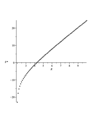
Figure 2: The coordinate $\rho^{*}$ takes the sonic horizon to $-\infty$, while preserving $+\infty$. In the figure, $R=r^{\prime}/2M$.

Notice that in order to build this plot (as well as that of the effective potential, see below), an explicit form of the background solution was needed. It was represented by the function

$$v=\frac{(f-1)^{2}}{1-a_{1}f}-a_{2}f,$$

where $a_{1}=0.8599$, and $a_{2}=0.0003$. This curve is in very good agreement with that obtained from Eqn.(19), as the plots in Fig. 1 show.

The effective potential $V_{\rm eff}$ in Eqn.(27) is given by

$$V_{\rm eff}=\frac{\ell(\ell+1)\sigma}{r^{\prime 2}G^{t^{\prime}t^{\prime}}}-\frac{1}{4}\left[\frac{1}{r^{\prime 2}}\frac{d}{d\rho^{*}}\left(\frac{r^{\prime 2}}{\sigma}\right)\right]^{2}-\frac{1}{2}\frac{d}{d\rho^{*}}\left[\frac{1}{r^{\prime 2}}\frac{d}{d\rho^{*}}\left(\frac{r^{\prime 2}}{\sigma}\right)\right],$$ (29)

where $\sigma\equiv\sqrt{M^{rt}-M^{tt}M^{rr}}$. This expression reduces to the usual one in the case of a linear theory for the scalar field, see for instance (Frolov1998, ). Fig. 3 displays the plot of $V_{\rm eff}(\rho^{*})$ for several values of the angular momentum $\ell$.

Figure 3: The effective potential as a function of $\rho^{*}$ for $\ell=0$ (bottom curve), $\ell=2$ (middle curve), and $\ell=5$.

As discussed for instance in (Wald1979, ), the positivity of the potential is sufficient to guarantee the stability of the sistem.

VI Conclusions

We have shown that the system composed of a Schwarzschild black hole accreting a steady-state and spherically symmetric ghost condensate described by the Lagrangian given in Eqn.(14) is linearly stable using two methods. The method developed by Moncrief consists in determining the sign of the time derivative of the energy of the perturbations through a surface integral, and led to the linear stability of the system in a few steps. This method profits from the symmetries of the system, and it does not use the explicit form of the solution for the scalar field. We have also shown that the system is linearly stable by the method of the effective potential but in this case, much longer calculations are involved, and an explicit form of the solution is required. Extensions of this work, currently under way, are the study of the nonlinear stability of the system (since linear stability is only a pre-requisite for full stability), and the generalization of Moncrief’s method to other Killing vectors.

- [1] Ratindranath Akhoury, David Garfinkle, and Ryo Saotome. Gravitational collapse of k-essence. JHEP, 1104:096, 2011.
- [2] Ratindranath Akhoury, David Garfinkle, Ryo Saotome, and Alexander Vikman. Non-Stationary Dark Energy Around a Black Hole. Phys.Rev., D83:084034, 2011.
- [3] Ratindranath Akhoury, Christopher S. Gauthier, and Alexander Vikman. Stationary Configurations Imply Shift Symmetry: No Bondi Accretion for Quintessence / k-Essence. JHEP, 0903:082, 2009.
- [4] Nima Arkani-Hamed, Hsin-Chia Cheng, Markus A. Luty, and Shinji Mukohyama. Ghost condensation and a consistent infrared modification of gravity. JHEP, 0405:074, 2004.
- [5] C. Armendariz-Picon, Viatcheslav F. Mukhanov, and Paul J. Steinhardt. A Dynamical solution to the problem of a small cosmological constant and late time cosmic acceleration. Phys.Rev.Lett., 85:4438–4441, 2000.
- [6] C. Armendariz-Picon, Viatcheslav F. Mukhanov, and Paul J. Steinhardt. Essentials of k essence. Phys.Rev., D63:103510, 2001.
- [7] E. Babichev, S. Chernov, V. Dokuchaev, and Yu. Eroshenko. Perfect fluid and scalar field in the Reissner-Nordstrom metric. J.Exp.Theor.Phys., 112:784–793, 2011.
- [8] E. Babichev, Viatcheslav F. Mukhanov, and A. Vikman. Escaping from the black hole? JHEP, 0609:061, 2006.
- [9] Eugeny Babichev, Viatcheslav Mukhanov, and Alexander Vikman. k-Essence, superluminal propagation, causality and emergent geometry. JHEP, 0802:101, 2008.
- [10] Carlos Barcelo, Stefano Liberati, and Matt Visser. Analog gravity from field theory normal modes? Class.Quant.Grav., 18:3595–3610, 2001.
- [11] Carlos Barcelo, Stefano Liberati, and Matt Visser. Analogue gravity. Living Rev.Rel., 8:12, 2005.
- [12] Neven Bilic. Relativistic acoustic geometry. Class.Quant.Grav., 16:3953–3964, 1999.
- [13] H. Bondi. On spherically symmetrical accretion. Monthly Notices of the Royal Astronomical Society, 112:195, 1952.
- [14] Andrei V. Frolov. Accretion of ghost condensate by black holes. Phys.Rev., D70:061501, 2004.
- [15] V.P. Frolov and I.D. Novikov. Black hole physics: Basic concepts and new developments. 1998.
- [16] A. R. Garlick. The stability of Bondi accretion. Astronomy & Astrophysics, 73:171–173, March 1979.
- [17] J. Garriga and V. F. Mukhanov. Perturbations in k-inflation. Physics Letters B, 458:219–225, July 1999.
- [18] E. Goulart and Santiago Esteban Perez Bergliaffa. Effective metric in nonlinear scalar field theories. Phys.Rev., D84:105027, 2011.
- [19] Alexander A. H. Graham and Rahul Jha. No-Hair Theorems in K-Essence Theories. 2014.
- [20] C. Danielle Leonard, Jonathan Ziprick, Gabor Kunstatter, and Robert B. Mann. Gravitational collapse of K-essence Matter in Painlevé-Gullstrand coordinates. JHEP, 1110:028, 2011.
- [21] P. Mach. On the stability of steady general-relativistic accretion and analogue black holes. Reports on Mathematical Physics, 64:257–269, August 2009.
- [22] P. Mach and E. Malec. Stability of relativistic Bondi accretion in Schwarzschild-(anti)-de Sitter spacetimes. Phys. Rev. D, 88(8):084055, October 2013.
- [23] I. Mandal, A. K. Ray, and T. K. Das. Critical properties of spherically symmetric black hole accretion in Schwarzschild geometry. Monthly Notices of the Royal Astronomical Society, 378:1400–1406, July 2007.
- [24] F. C. Michel. Accretion of Matter by Condensed Objects. Astrophysics & Space Science, 15:153–160, January 1972.
- [25] V. Moncrief. Odd-parity stability of a Reissner-Nordström black hole. Phys. Rev. D, 9:2707–2709, May 1974.
- [26] V. Moncrief. Stability of Reissner-Nordström black holes. Phys. Rev. D, 10:1057–1059, August 1974.
- [27] V. Moncrief. Stability of stationary, spherical accretion onto a Schwarzschild black hole. Astrophys. J. , 235:1038–1046, February 1980.
- [28] In all these publications, the fluid was taken as non-gravitating. For general-relativistic spherically symmetric steady accretion of self-gravitating perfect fluid onto compact objects see [21].
- [29] This method was recently used to study the stability of stationary, relativistic Bondi-type accretion in Schwarzschild anti deSitter spacetimes [22].
- [30] J. A. Petterson, J. Silk, and J. P. Ostriker. Variations on a spherically symmetrical accretion flow. Monthly Notices of the Royal Astronomical Society, 191:571–579, May 1980.
- [31] T. Regge and J. A. Wheeler. Stability of a Schwarzschild Singularity. Physical Review, 108:1063–1069, November 1957.
- [32] Robert J. Scherrer. Purely kinetic k-essence as unified dark matter. Phys.Rev.Lett., 93:011301, 2004.
- [33] Shinji Tsujikawa. Dark energy: investigation and modeling. 2010.
- [34] R. M. Wald. Note on the stability of the Schwarzschild metric. Journal of Mathematical Physics, 20:1056–1058, June 1979.
- [35] B. F. Whiting. Mode stability of the Kerr black hole. Journal of Mathematical Physics, 30:1301–1305, June 1989.