Error distributions on large entangled states with non-Markovian dynamics

Abstract

We investigate the distribution of errors on a computationally useful entangled state generated via the repeated emission from an emitter undergoing strongly non-Markovian evolution. For emitter-environment coupling of pure-dephasing form, we show that the probability that a particular patten of errors occurs has a bound of Markovian form, and thus accuracy threshold theorems based on Markovian models should be just as effective. Beyond the pure-dephasing assumption, though complicated error structures can arise, they can still be qualitatively bounded by a Markovian error model.

The theoretical and technical challenges faced in the construction of a quantum computer have rightly brought into light the question of the scalability of such a device Unruh (1995); Alicki et al. (2002, 2006); Alicki ; Kalai . There is, however, cause for optimism, since accuracy threshold theorems imply that quantum computation should be achievable to arbitrary precision Aharonov and Ben-Or (1998); Knill et al. (1998); Preskill (1998); Aliferis et al. (2005); Terhal and Burkard (2005); Aharonov et al. (2006); Preskill (2013). The existence of such thresholds relies on quantum error correction codes Shor (1995); Steane (1995); Laflamme et al. (1996), and that the noise afflicting the computation device satisfies certain conditions on its strength, and level of spatial and temporal correlations. In particular, the first theoretical achievements assumed Markovian and independent noise afflicting the components of the quantum computer Aharonov and Ben-Or (1998); Knill et al. (1998); Preskill (1998), the intuition being that, typically, the components of the device reside in different locations, and that the (local) environments causing the errors are large enough that they have an effectively negligible memory time Breuer and Petruccione (2002).

While these assumptions will be valid in some quantum systems, whether they are valid for those systems able to perform quantum computations remains to be seen. Recently, prompted by a debate between Kalai and Harrow, considerable discussion has taken place in the community about some of the core assumptions of the error models underpinning threshold theorems for fault tolerant quantum computing Kalai ; Preskill (2013); Galai and Harrow (2012); Flammia and Harrow (2013). Broadly speaking, questions have been raised about the spatial and temporal structure of errors incurred when one creates large entangled states without the usual assumption of Markovian dynamics.

The purpose of this work is twofold: In the first instance, we analyse a worst-case scenario, wherein a large photonic cluster state Raussendorf and Briegel (2001); Raussendorf et al. (2003) is created by a single emitter that is continuously coupled to an environment in a highly non-Markovian manner. In this scenario, it is reasonable to believe that all the errors on this photonic state arise from the emission process, as once the photons are travelling in free space they are effectively decoherence-free. Secondly, we analyse this procedure in the context of a specific experimental proposal with realistic parameters, where the emitter is a charged quantum dot interacting with a nuclear spin bath. As our main result, we show that one can obtain a bound on the non-Markovian error distribution probabilities which has a Markovian form. Crucially, this means that methods for combating Markovian errors will work just as efficiently in this highly non-Markovian situation. When the emitter is subject to pure-dephasing noise - as can be the case for the proposal we consider - our bound is analytically derived. Outside this regime, the structure of errors becomes more complicated, though we show numerically how a Markovian error model can still correctly capture all features and provide a tight bound.

In order to give a context, we phrase our augments in terms of the linear cluster proposal of Ref. Lindner and Rudolph (2009), which consists of the repeated absorption and reemission of a string of photons from a quantum dot (QD) residing in a magnetic field perpendicular to the growth direction . We note that there are practical proposals (with experiments underway) to build such devices Lindner and Rudolph (2009); Li et al. (2011); Economou et al. (2010); Lin and He (2010), though we emphasise that our analysis equally applies to any cluster state produced in a similar manner. In the ideal case (no coupling to an environment), a state of $n$ entangled photons and the QD, $\left|\mathcal{C}_{n}\right\rangle$, is generated from an initially separable state via [see Fig. (1)]:

$$\left|\mathcal{C}_{n}\right\rangle=\left[\prod_{i=1}^{n}(C_{i}U_{y})\right]\left|0\right\rangle_{D}\left|0\dots 0\right\rangle$$ (1)

where $\left|0\right\rangle_{D}\equiv\left|\uparrow\right\rangle$ ($\left|1\right\rangle_{D}\equiv\left|\downarrow\right\rangle$) is the state of the QD aligned (anti-aligned) along the z-axis, $\left|0\dots 0\right\rangle\equiv\bigotimes_{i=1}^{n}\left|R\right\rangle$ represents the initial state of the $n$-photons all having right circular polarisation, $C_{i}=\left|0\right\rangle\hskip-2.84526pt\left\langle 0\right|_{D}\otimes\openone_{i}+\left|1\right\rangle\hskip-2.84526pt\left\langle 1\right|_{D}\otimes X_{i}$ is a CNOT gate on the QD and the ith photon representing an absorption and emission process, and $U_{y}=\mathrm{e}^{-iY_{D}\pi/4}$ rotates the QD about the y-axis. Our basis is such that $Z_{D}=\left|0\right\rangle\hskip-2.84526pt\left\langle 0\right|_{D}-\left|1\right\rangle\hskip-2.84526pt\left\langle 1\right|_{D}$ and $Z_{i}=\left|0\right\rangle\hskip-2.84526pt\left\langle 0\right|_{i}-\left|1\right\rangle\hskip-2.84526pt\left\langle 1\right|_{i}$ where $\left|1\right\rangle_{i}\equiv\left|L\right\rangle_{i}$.

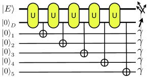
Figure 1: Quantum circuit for the generation of a linear cluster state of five photons and a quantum dot. Non-Markovian decoherence of the dot is modelled as a sequential coupling to an environment. In the ideal case the unitaries are replaced by $\mathrm{e}^{-iY_{D}\pi/4}\otimes\openone_{E}$.

Non-Markovian evolution of the QD is introduced by sequentially coupling it to an environment such that $U_{y}\to U$, with $U$ acting on the QD and its environment.

Before we do so, we first simply consider the effect of Pauli errors on the QD before, say, the emission of photon $l$, i.e. we insert $X_{D}$, $Y_{D}$, or $Z_{D}$ to the left of $C_{l-1}$ in Eq. (1). We refer to this type of error (on the QD itself as apposed to the resulting photon state) as a fundamental error. We find that $\left|\mathcal{C}_{n}\right\rangle$ becomes $Z_{l}\left|\mathcal{C}_{n}\right\rangle$, $Z_{l}Z_{l-1}\left|\mathcal{C}_{n}\right\rangle$, and $Z_{l-1}\left|\mathcal{C}_{n}\right\rangle$, for $X_{D}$, $Y_{D}$, and $Z_{D}$ respectively . Thus, we see that imperfections in the evolution of the QD (fundamental errors), are mathematically equivalent to localised errors on the resulting photon state Lindner and Rudolph (2009).

We now investigate how these errors are distributed. We assume that the absorption and emission processes of the photons occur on a timescale far shorter than the rotations of the QD, and the CNOT gates are therefore treated as being instantaneous. It was shown in Ref. Lindner and Rudolph (2009) that relaxation of this assumption gives rise to photons with wave-packets which correspond to a fixed probability of a fundamental Y error on the QD for each CNOT gate. To model the non-Markovian evolution of the QD we replace $U_{y}$ in Eq. (1) with the general operator $U=\left|0\right\rangle\hskip-2.84526pt\left\langle 0\right|_{D}A_{00}+\left|0\right\rangle\hskip-2.84526pt\left\langle 1\right|_{D}A_{01}+\left|1\right\rangle\hskip-2.84526pt\left\langle 0\right|_{D}A_{10}+\left|1\right\rangle\hskip-2.84526pt\left\langle 1\right|_{D}A_{11}$, where the operators $A_{00}$ etc. act on the environment $\left|E\right\rangle$. Eq. (1) becomes $\left|\Psi_{n}\right\rangle=\left[\prod_{i=1}^{n}(C_{i}U)\right]\left|0\right\rangle_{D}\left|0\dots 0\right\rangle\left|E\right\rangle$, which inspection reveals can be written

$$\left|\Psi_{n}\right\rangle=\sum_{\boldsymbol{b}}\left|b_{n}\right\rangle_{D}\left|\boldsymbol{b}\right\rangle\mathcal{F}(\boldsymbol{b})\left|E\right\rangle$$ (2)

where $\boldsymbol{b}=(b_{n}b_{n-1}\dots b_{2}b_{1})$ with $b_{i}\in\{0,1\}$ a bit string, $\mathcal{F}(\boldsymbol{b})=A_{b_{n}b_{n-1}}A_{b_{n-1}b_{n-2}}\dots A_{b_{2}b_{1}}A_{b_{1}0}$ is a product of environment operators, and the sum runs over all $2^{n}$ possible bit-strings $\boldsymbol{b}$. Eq. (2) is the complete state of the QD, $n$ photons and environment. Now, we denote by $P(\boldsymbol{\alpha})$, where $\boldsymbol{\alpha}=(\alpha_{n}\alpha_{n-1}\dots\alpha_{2}\alpha_{1})$ with $\alpha_{i}\in\{0,1\}$, the probability that the photonic state is measured having Pauli $Z$ errors on those photons for which $\alpha_{i}=1$, i.e. the state $\left|\Phi(\boldsymbol{\alpha})\right\rangle=[\prod_{i=1}^{n}Z_{i}^{\alpha_{i}}]\left|\mathcal{C}_{n}\right\rangle$. We find $P(\boldsymbol{\alpha})=\left\langle\Phi(\boldsymbol{\alpha})\right|{\rm{Tr}}_{E}(\left|\Psi_{n}\right\rangle\hskip-2.84526pt\left\langle\Psi_{n}\right|)\left|\Phi(\boldsymbol{\alpha})\right\rangle=\mathrm{Tr}_{E}(O(\boldsymbol{\alpha})^{\dagger}O(\boldsymbol{\alpha})\left|E\right\rangle\hskip-2.84526pt\left\langle E\right|)$, where the environment operator $O(\boldsymbol{\alpha})=\sqrt{2}\left\langle+\right|_{D}W(\boldsymbol{\alpha})\left|0\right\rangle_{D}$ is a matrix element of the QD–environment operator

$$W(\boldsymbol{\alpha})=\prod_{i=1}^{n}(Z^{\alpha_{i}}\Delta)=(Z^{\alpha_{n}}\Delta)\dots(Z^{\alpha_{1}}\Delta),$$ (3)

with $\left|+\right\rangle_{D}=(1/\sqrt{2})(\left|0\right\rangle_{D}+\left|1\right\rangle_{D})$, $Z=Z_{D}\otimes\openone_{E}$, and $\Delta=(1/\sqrt{2})(U-2\left|0\right\rangle\hskip-2.84526pt\left\langle 0\right|_{D}U\left|1\right\rangle\hskip-2.84526pt\left\langle 1\right|_{D})$ is a non-unitary operator acting in the joint QD-environment Hilbert space. For the probability of zero errors, for example, we have the scalar $P(\boldsymbol{0})=\mathrm{Tr}_{E}(O(\boldsymbol{0})^{\dagger}O(\boldsymbol{0})\left|E\right\rangle\hskip-2.84526pt\left\langle E\right|)$, which depends on the environment operator $O(\boldsymbol{0})=\sqrt{2}\left\langle+\right|_{D}W(\boldsymbol{0})\left|0\right\rangle_{D}$, which, from Eq. (3), in turn depends on the QD-environment operator $W(\boldsymbol{0})=\Delta^{n}$. For the probability of an error on, say, photon $l$, the relevant operator is $W(0\dots 010\dots 0)=\Delta^{n-l}Z\Delta^{l}$, and so on. Thus, calculating the probability of a given error distribution amounts to calculating products of $Z$ and the non-Hermitian matrix $\Delta$. Eq. (3) provides us with a systematic way to determine error distribution probabilities in the non-Markovian case, making no assumptions about the state of the environment, its memory timescale, or its interaction strength with, or potential correlations with, the QD at any point in the evolution. Though we have phrased our analysis in terms of quantum dots and photons, Eq. (3) is valid for any cluster state generated as shown in Fig. (1).

For emitter–environment coupling of pure-dephasing form, Eq. (3) can be further simplified. We motivate this by noting that for electrons in QDs, the dominant source of dephasing is due to coupling to nuclear spins via hyper-fine interactions Cywiński et al. (2009a, b); Coish et al. (2010); Barnes et al. (2012). Since we consider a field in the $y$-direction, the Hamiltonian takes the form $H=(\Omega/2)Y_{D}+(1/2)\sum_{k}\omega_{k}I_{k}^{y}+(1/4)\sum_{k}A_{k}\boldsymbol{S}\cdot\boldsymbol{I}_{k}+H_{\mathrm{dip}}$, where $\boldsymbol{S}=(X_{D},Y_{D},Z_{D})$, while $\boldsymbol{I}_{k}=(I_{k}^{x},I_{k}^{y},I_{k}^{z})$ acts on environment spin $k$, and $H_{\mathrm{dip}}=\sum_{k\neq k^{\prime}}b_{kk^{\prime}}(I_{k}^{+}I_{k^{\prime}}^{-}-(1/2)I_{k}^{y}I_{k^{\prime}}^{y})$ with $I_{k}^{\pm}=(1/2)(I_{k}^{x}\pm iI_{k}^{z})$. Typically, the Zeeman energy of the QD spin is far larger than those of the nuclei, leading to a suppression of relaxation processes. The quantity regulating this distinction is $\delta=\mathcal{A}/(\Omega\sqrt{N}$), where $\mathcal{A}=\sum_{k}A_{k}$ and $N$ is the number of nuclei appreciably interacting with the QD spin. For $\delta\ll 1$, it was shown that the full Hamiltonian above can be approximated by the pure-dephasing Hamiltonian Cywiński et al. (2009a, b) $H_{\mathrm{PD}}=(\Omega_{\mathrm{eff}}/2)Y_{D}+\left|+i\right\rangle\hskip-2.84526pt\left\langle+i\right|H_{+}+\left|-i\right\rangle\hskip-2.84526pt\left\langle-i\right|H_{-}$ where $Y_{D}\left|\pm i\right\rangle=\pm\left|\pm i\right\rangle$ and $H_{\pm}=\mp(1/2)\langle B_{N}\rangle+(1/2)\sum_{k}(\omega_{k}^{\prime}\pm{\textstyle{\frac{1}{2}}}A_{k})I_{k}^{y}\pm(1/4)\sum_{k\neq k^{\prime}}\frac{A_{k}A_{k^{\prime}}}{\Omega}I_{k}^{+}I_{k^{\prime}}^{-}+H_{\mathrm{dip}}$, with $\omega_{k}^{\prime}=\omega_{k}-A_{k}^{2}/(4\Omega)$. The effective magnetic field is $\Omega_{\mathrm{eff}}=\Omega+\langle B_{N}\rangle+(1/4)\sum_{k}A_{k}^{2}/\Omega$ where $\langle B_{N}\rangle=\mathrm{Tr}(B_{N}\rho_{E})$ with $B_{N}=(1/2)\sum_{k}A_{k}I_{k}^{y}$ the Overhauser field operator. For typical GaAs QDs the total coupling strength $\mathcal{A}\sim 1~{}$T, while the typical values of N range from $10^{4}$ to $10^{6}$ Cywiński et al. (2009a, b); Coish et al. (2010). Thus, field strengths of $\Omega\sim 100$ mT and above should be well described by the pure-dephasing Hamiltonian.

Using $U=\exp[-i\pi/(2\Omega_{\mathrm{eff}})H_{\mathrm{PD}}]$, from Eq. (3) we find for a general error distribution $\boldsymbol{\alpha}$ we have

$$O(\boldsymbol{\alpha})=\prod_{i=1}^{n}\frac{\sqrt{(-1)^{f_{i}(\boldsymbol{\alpha})}}}{2}\Big{[}U_{-}+(-1)^{f_{i}(\boldsymbol{\alpha})}U_{+}\Big{]}$$ (4)

with $f_{i}(\boldsymbol{\alpha})=\sum_{j=i}^{n}\alpha_{j}$ and $U_{\pm}=\exp[-i(\pi/2\Omega_{\mathrm{eff}})H_{\pm}]$. We see that $O(\boldsymbol{\alpha})$ consists of a product of $n$ operators, each of which being either $M_{\pm}=(\sqrt{\pm 1}/2)(U_{-}\pm U_{+})$ depending on the error distribution $\boldsymbol{\alpha}$. Using Eq. (4), and the sub-multiplacative property of the operator norm defined as $||A||\equiv\mathrm{max}_{\left|\phi\right\rangle}\left\langle\phi\right|A\left|\phi\right\rangle/\langle\phi|\phi\rangle$, we find the non-Markovian error probabilities satisfy

$$P(\boldsymbol{\alpha})\leq||M_{-}^{\dagger}M_{-}||^{h(\boldsymbol{\alpha})}||M_{+}^{\dagger}M_{+}||^{n-h(\boldsymbol{\alpha})}$$ (5)

where $h(\boldsymbol{\alpha})=\frac{1}{2}(n-\sum_{i=1}^{n}(-1)^{f_{i}(\boldsymbol{\alpha})})$ is the number of occurrences of $M_{-}$ in Eq. (4). We see that $||M_{-}^{\dagger}M_{-}||$ plays the role of an error probability, with unitarity of $U_{\pm}$ ensuring that $||M_{\pm}^{\dagger}M_{\pm}||\leq 1$. Note that $h(\boldsymbol{\alpha})$ does not count the number of errors on the photonic state: it counts the number of adjacent pairs necessary to create it, or equivalently, the number of fundamental QD errors. The form of $H_{\mathrm{PD}}$ means that the environment can only induce fundamental Y errors on the QD, which make adjacent pairs of errors on the resulting photonic cluster state. A single isolated error, say $\boldsymbol{\alpha}=(010)$, has $h(010)=2$, since pairs of adjacent errors at positions $1$ and $2$ are required to realise it.

Eq. (5) shows that even in the non-Markovian case, we can put a rigorous bound on the probability of a given error distribution, which behaves as a power law in the number of fundamental errors in the distribution. More importantly, we see that the non-Markovian nature of the environment cannot introduce long range spatial correlations in the errors; the probability of $h$ fundamental errors is bounded by $p_{-}^{h}$ with $\smash{p_{-}=||M_{-}^{\dagger}M_{-}||\leq 1}$. These results are valid for any cluster state generated in the way shown in Fig. (1) when the emitter-environment coupling takes on a pure-dephasing form.

For the QD example we consider, we can go further by noticing that the total spin projection in the $y$-direction is conserved, $[H_{\pm},\sum_{k}I_{k}^{y}]=0$. The operators $U_{\pm}=\exp[-i(\pi/2\Omega_{\mathrm{eff}})H_{\pm}]$ from which the probabilities are calculated are therefore block-diagonal, and the result is that the probabilities become a sum over contributions from spaces with fixed spin projections. By defining projection operators $\mathcal{P}_{m}$ which satisfy $\sum_{m}\mathcal{P}_{m}=\openone_{E}$ and project onto the eigenspace with eigenvalue of $\sum_{k}I_{k}^{y}$ equal to $m$, the probabilities can be written $P(\boldsymbol{\alpha})=\sum_{m}P_{m}(\boldsymbol{\alpha})$ where $P_{m}(\boldsymbol{\alpha})=\mathrm{Tr}_{E}(O_{m}^{\dagger}(\boldsymbol{\alpha})O_{m}(\boldsymbol{\alpha})\rho_{m})$, and $\rho_{m}$ is the environment state in the $m$ subspace, while $O(\boldsymbol{\alpha})=\mathcal{P}_{m}O(\boldsymbol{\alpha})\mathcal{P}_{m}$. In this way, we can make use of properties we know of the environment state. For example, for an initial environment state having weight in a single $m$ sector only, we can write $P(\boldsymbol{\alpha})=P_{m}(\boldsymbol{\alpha})$ and bound by

$$P_{m}(\boldsymbol{\alpha})\leq||M_{-}^{(m)\dagger}M_{-}^{(m)}||^{h(\boldsymbol{\alpha})}||M_{+}^{(m)\dagger}M_{+}^{(m)}||^{n-h(\boldsymbol{\alpha})}$$ (6)

where $M_{\pm}^{(m)}=\mathcal{P}_{m}M_{\pm}\mathcal{P}_{m}$. This bound is tighter than that given in Eq. (5) since the operators involved necessarily act non-trivially in a smaller space.

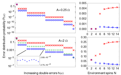
Figure 2: Left panels: all $2^{5}$ non-Markovian error distribution probabilities for a 5-photon state, calculated exactly (blue circles), using the bound given in Eq. (6) (red crosses), and a best-fit to a Markovian model of the form $p^{h}(1-p)^{n-h}$ (green circles). The error distributions are ordered along the $x$-axis such that those corresponding to the least number of fundamental errors are to the left. The inset in the lower plot shows a zoom in of the $h(\boldsymbol{\alpha})=2$ band. Right panels: scaling of a typical error distribution probability with increasing environment size.

In Fig. (2) we plot the exact non-Markovian error probabilities (blue circles) and the bound calculated using Eq. (6) (red crosses), using the pure-dephasing Hamiltonian. The left panels show all $2^{5}$ error probabilities for a $5$-photon state, ordered by increasing fundamental errors, $h(\boldsymbol{\alpha})$, for an environment of $N=10$ spins initially in an equal mixture in the $m=0$ subspace . The probabilities fall into distinct bands determined by their value of $h(\boldsymbol{\alpha})$, and the bounds correctly capture the behaviour of the exact values. For small $\mathcal{A}/\Omega$ our bound is relatively tight, while for $\mathcal{A}/\Omega=2$ where our derived bound gives fairly high values, the exact probabilities are still well behaved and remain low. In fact, they can be bounded using a simple best-fit procedure by a Markovian model of the form $p^{h}(1-p)^{n-h}$, with $p$ significantly less than $p_{-}$, as show in green on the lower left plot. It is clear from Fig. (2) that the non-Markovian errors do not show harmful long-range correlations, as the bound suggests. Thus, strategies to combat errors assuming Markovian evolution will, in this regime, remain effective in the non-Markovian case.

Note that we have chosen here an initial environment state for which the average Overhauser field is zero $\langle B_{N}\rangle=0$, and for which fluctuations are small, $\Delta B_{N}=\sqrt{\langle(B_{N})^{2}\rangle-\langle B_{N}\rangle^{2}}\ll\Omega$. As a result, dephasing due to ensemble average over the Zeeman field is eliminated, and the error probabilities remain low and approximately equal. Importantly, as long as the initial state obeys $\Delta B_{N}\ll\Omega$, the features seen in Fig. (2) are remarkably robust; since we include $\langle B_{N}\rangle$ in $\Omega_{\mathrm{eff}}$, they are also present in cases for which $\langle B_{N}\rangle\neq 0$, including initially pure environment states.

In the right panels of Fig. (2) we show the scaling with increasing environment size of the exact probability and the bound in Eq. (6), for a typical error distribution $\boldsymbol{\alpha}=(01100)$ for which $h(\boldsymbol{\alpha})=1$. With pure-dephasing, the exact probabilities ought to scale as $\sim 1-(1+|a|\,N^{-2})^{-1/2}$ where $a$ is fixed for fixed $\mathcal{A}$ and $\Omega$ Cywiński et al. (2009a, b), and we find that the bound obeys a similar scaling $\sim c-(1-|a|\,N^{-2})^{-1/2}$. The dashed lines show fits of this form, showing that the probabilities and bound scale as expected with $N$. Thus, the bound we derive tends to a constant value with increasing environment size, and for small $\mathcal{A}/\Omega$, can directly replace the error rate in threshold theorems assuming Markovian error models. In fact, even when $\mathcal{A}/\Omega$ takes on higher values, our numerics strongly suggest that one can tightly bound the error distribution with a Markovian model.

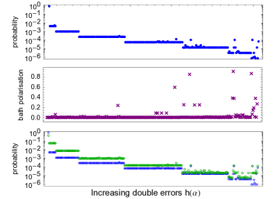
Figure 3: Top: all $2^{8}$ exact non-Markovian error probabilities for a 8 photon state in the non-pure-dephasing case. Middle: corresponding polarisation $\langle\sum_{k}I_{k}^{y}\rangle$ of the spin environment: error probabilities falling outside their bands correspond to angular momentum exchanges. Bottom: the qualitative features of the probability distribution can be captured by a simple Markovian model shown in green.

For typical QDs the pure-dephasing form is valid for magnetic field strengths of $\sim 100$ mT and above. However, for optimal performance of the specific cluster state proposal we consider Lindner and Rudolph (2009) smaller magnetic fields would be preferred (though not essential). To investigate this regime, in the top panel of Fig. (3) we show the non-Markovian probabilities calculated using the full hyper-fine Hamiltonian, for an 8 photon state with $\mathcal{A}/\Omega=4$ and $N=6$ such that $\delta\approx 1.6$ (so that $\Omega\sim 1~{}\mathrm{mT}$ for realistic QD sizes). We see that the band structure becomes convolved with probabilities that lie above their bands. These distributions all have the form $\boldsymbol{\alpha}_{1}=(\dots 1\dots)$; the Hamiltonian we now use can induce fundamental X and Z errors on the QD, which correspond to single errors on the photon state. This can be further understood in the middle panel, where we show the corresponding polarisation of the environment $\langle\sum_{k}I_{k}^{y}\rangle$ for each distribution; when a distribution of the form $\boldsymbol{\alpha}_{1}$ is realised, angular momentum is exchanged with the environment.

Though these exact non-Markovian probabilities appear to have a more complicated structure, they can still be qualitatively described by a Markovian model. With any error distribution $\boldsymbol{\alpha}$ we can associate a finite number of QD trajectories which will result in it. An error distribution $\boldsymbol{\alpha}_{1}$, for example, can be made from a combination of fundamental Y errors, or a single X or Z error. We can therefore define a simple Markovian model, wherein we assign fixed probabilities for fundamental $X$, $Y$, and $Z$ errors, from these calculate the probability of a given trajectory, and sum over all trajectories corresponding to a given error distribution. Probabilities calculated in this way are shown in green in the lower panel of Fig. (3). Importantly, we see that these Markovian error probabilities qualitatively capture all the exact non-Markovian probabilities.

We have investigated the distribution of errors on a large entangled state generated by the repeated emission from a single emitter with non-Markovian evolution. For pure-dephasing dynamics, we found that the error probabilities have a bound of Markovian form, such that error correction schemes remain just as effective in this non-Markovian regime. We have also shown that the errors can be bounded by a Markovian model even beyond pure-dephasing dynamics, suggesting the board applicability of our findings.

Acknowledgments - The authors wish to thank Sophia Economou and John Preskill for numerous useful discussions. D.P.S.M. acknowledges CONICET and SIQUTE (Contract No. EXL02) of the European Metrology Research Programme (EMRP) for support. The EMRP is jointly funded by the EMRP participating countries with EURAMET and the European Union. N.H.L. thanks the Israel Excellence Centre “Circle of Light”. T.R. is supported by the Vienna Science and Technology Fund (WWTF, Grant No. ICT 12-041), and the Army Research Office (ARO) Grant No. W911NF-14-1-0133. D.P.S.M. and T.R. also acknowledge support from the EPSRC and CHIST-ERA project SSQN.

References

- Unruh (1995) W. G. Unruh, Phys. Rev. A 51, 992 (1995).
- Alicki et al. (2002) R. Alicki et al., Phys. Rev. A 65, 062101 (2002).
- Alicki et al. (2006) R. Alicki, D. A. Lidar, and P. Zanardi, Phys. Rev. A 73, 052311 (2006).
- (4) R. Alicki, arXiv:quant-ph/0411008 (2004).
- (5) G. Kalai, arXiv:quant-ph/1106.0485 (2011), arXiv:quant-ph/0904.3265 (2009), arXiv:quant-ph/0806.2443 (2008), arXiv:quant-ph/0607021 (2006), arXiv:quant-ph/0508095 (2005).
- Aharonov and Ben-Or (1998) D. Aharonov and M. Ben-Or, Proc. 29th Ann. ACM Symp. on Theory of Computing p. 179 (1998).
- Knill et al. (1998) E. Knill, R. Laflamme, and W. H. Zurek, Proc. Roy. Soc. London, Ser. A 454, 365 (1998).
- Preskill (1998) J. Preskill, Proc. Roy. Soc. London, Ser. A 454, 385 (1998).
- Aliferis et al. (2005) P. Aliferis, D. Gottesman, and J. Preskill (2005), quant-ph/0504218.
- Terhal and Burkard (2005) B. M. Terhal and G. Burkard, Phys. Rev. A 71, 012336 (2005).
- Aharonov et al. (2006) D. Aharonov, A. Kitaev, and J. Preskill, Phys. Rev. Lett. 96, 050504 (2006).
- Preskill (2013) J. Preskill, Quant. Inf. Comput. 13, 181 (2013).
- Shor (1995) P. W. Shor, Phys. Rev. A 52, 2493 (1995).
- Steane (1995) A. M. Steane, Phys. Rev. Lett. 77, 793 (1995).
- Laflamme et al. (1996) R. Laflamme et al., Phys. Rev. Lett. 77, 198 (1996).
- Breuer and Petruccione (2002) H.-P. Breuer and F. Petruccione, The Theory of Open Quantum Systems (Oxford University Press, 2002).
- Galai and Harrow (2012) R. Galai and A. Harrow (2012), URL http://rjlipton.wordpress.com/2012/01/30/.
- Flammia and Harrow (2013) S. T. Flammia and A. W. Harrow, Q. Inf. & Comp. 13, 1 (2013).
- Raussendorf and Briegel (2001) R. Raussendorf and H. J. Briegel, Phys. Rev. Lett. 86, 5188 (2001).
- Raussendorf et al. (2003) R. Raussendorf, D. E. Browne, and H. J. Briegel, Phys. Rev. A 68, 022312 (2003).
- Lindner and Rudolph (2009) N. H. Lindner and T. Rudolph, Phys. Rev. Lett. 103, 113602 (2009).
- Li et al. (2011) Y. Li, L. Aolita, and L. C. Kwek, Phys. Rev. A 83, 032313 (2011).
- Economou et al. (2010) S. E. Economou, N. Lindner, and T. Rudolph, Phys. Rev. Lett. 105, 093601 (2010).
- Lin and He (2010) Q. Lin and B. He, Phys. Rev. A 82, 022331 (2010).
- Cywiński et al. (2009a) Ł. Cywiński, W. M. Witzel, and S. D. Sarma, Phys. Rev. B 79, 245314 (2009a).
- Cywiński et al. (2009b) Ł. Cywiński, W. M. Witzel, and S. D. Sarma, Phys. Rev. Lett 102, 057601 (2009b).
- Coish et al. (2010) W. A. Coish, J. Fischer, and D. Loss, Phys. Rev. B 81, 165315 (2010).
- Barnes et al. (2012) E. Barnes, Ł. Cywiński, and S. D. Sarma, Phys. Rev. Lett. 109, 140403 (2012).
- Browne and Rudolph (2005) D. E. Browne and T. Rudolph, Phys. Rev. Lett. 95, 010501 (2005).