SLAC–PUB–15920

Non-global Logarithms
at 3 Loops, 4 Loops, 5 Loops and Beyond

Matthew D. Schwartz⁽¹⁾, Hua Xing Zhu^(2)
(1)Center for the Fundamental Laws of Nature, Harvard University
⁽²⁾SLAC National Accelerator Laboratory, Stanford University, Stanford, CA 94309, USA

E-mails: schwartz@physics.harvard.edu, hxzhu@slac.stanford.edu

Abstract

We calculate the coefficients of the leading non-global logarithms for the hemisphere mass distribution analytically at $3$, $4$, and $5$ loops at large $N_{c}$. We confirm that the integrand derived with the strong-energy-ordering approximation and fixed-order iteration of the Banfi-Marchesini-Syme (BMS) equation agree. Our calculation exploits a hidden ${\rm PSL}(2,\mathbb{R})$ symmetry associated with the jet directions, apparent in the BMS equation after a stereographic projection to the Poincaré disk. The required integrals have an iterated form, leading to functions of uniform transcendentality. This allows us to extract the coefficients, and some functional dependence on the jet directions, by computing the symbols and coproducts of appropriate expressions involving classical and Goncharov polylogarithms. Convergence of the series to a numerical solution of the BMS equation is also discussed.

1 Introduction

Jet substructure is playing an increasingly prominent role in the physics of hadron collisions, particularly at the LHC [1, 2, 3, 4, 5, 6, 7, 8]. As new substructure methods are developed, it will be important to cross check the approximations used in Monte Carlo simulations both against data and against independent precision calculations in QCD. Such substructure calculations necessarily involve resummation of large logarithms. For sufficiently inclusive observables, this resummation is relatively straightforward. For example, traditional jet mass and shape distribution have been studied in great detail, both at $e^{+}e^{-}$ colliders [9, 10, 11, 12, 13, 14, 15, 16, 17, 18, 19] and hadron colliders [20, 21, 22, 23, 24, 25, 26, 27, 28, 29, 30, 31, 32, 33, 34, 35, 36]. However, for calculations involving multiple scales and parameters, such as with extra electroweak gauge bosons, jet vetoes, or jet algorithm parameters, it is less clear how to guarantee that all the relevant large logarithms are resummed. One particular challenge is to understand non-global logarithms (NGLs) [37, 38, 39, 40, 41, 42, 43].

Non-global logarithms were first characterized and understood by Dasgupta and Salam (DS)  [37]. They arise in exclusive observables for which phase space cuts unequally distribute the real and virtual contributions. Consider for example, the doubly differential distribution in hemisphere masses, $\frac{d^{2}\sigma}{dm_{L}dm_{R}}$ in an $e^{+}e^{-}$ collision [14, 15]. In certain limits, such as when $m_{L}\gg m_{R}$ (or vice versa), NGLs of the form $L=\left|\ln\frac{m_{L}}{m_{R}}\right|$ can give large contributions to the distribution. The leading dependence of the hemisphere mass cross section on $L$ (of order $\alpha_{s}^{2}L^{2}$), was computed in [37]. Subleading NGLs (of order $\alpha_{s}^{2}L$) were first computed in [14, 15]; these calculations also revealed surprising [44] non-logarithmic dependence on the non-global ratio $\frac{m_{L}}{m_{R}}$.

Whether NGLs provide a quantitatively important contribution to precision calculations, and whether they must be resummed, is only beginning to be understood [13, 17, 26, 28, 30]. Although global logarithms in substructure observables can be resummed using the renormalization group, for example using Soft-Collinear Effective Theory [45, 46, 47], it is not known how (or if) NGLs can be resummed using similar methods. Fortunately, the leading NGLs (terms of the form $(\alpha L)^{n}$) can be reproduced within the strong-energy-ordering approximation to QCD. This approximation leads to simplified cross sections, particularly at large $N_{c}$, and allows for straightforward resummation using Monte-Carlo (MC) simulation [37]. As an alternative to the MC approach, Banfi, Marchesini and Syme (BMS) have derived, using the same approximations, integro-differential equation [40], which describes the evolution of leading NGLs at large $N_{c}$. Remarkably, the BMS equation is mathematically similar to the Balitsky-Kovchegov (BK) equation describing the dynamics of gluon saturation at small $x$ [48, 49]. Based on this formal similarity, a finite $N_{c}$ generalization of BMS equation has been proposed in Ref. [50], and numerically studied in Ref. [51].

The BMS equation has the potential not just to resum the NGLs, but also to give us insights into their structure and importance. An interesting feature of this equation is that it has a hidden ${\rm PSL}(2,\mathbb{R})$ symmetry. More precisely, let us define the hemispheres with respect to the $n$ direction. Then consider the contribution $g_{ab}(L)$ to the right-hemisphere-mass distribution from a dipole, that is a pair of rapidly moving colored particles, in the $a$ and $b$ directions (neither of which are necessarily aligned with the left-hemisphere axis $\bar{n}^{\mu}$). While one would naturally expect cylindrical symmetry as $a$ and $b$ rotate around the hemisphere axis, there is actually a much larger ${\rm PSL}(2,\mathbb{R})$ symmetry acting on $a$ and $b$.

To calculate the $n$-loop leading NGL, we can iterate the BMS equation to produce the correct integrand. This iteration is equivalent to, but significantly simpler then, summing the relevant real, virtual, and real-virtual contributions in the strongly ordered limit and then subtracting the global contribution. Exploiting the ${\rm PSL}(2,\mathbb{R})$ symmetry, the calculation of $g_{ab}(L)$ for arbitrary $a$ and $b$ simplifies. Furthermore, since the integrands have an iterated structure, we can exploit the technology of symbols and coproducts to simplify expressions involving polylogarithms. Our final result for the leading NGL at 5 loops is

$$g_{n\overline{n}}({\widehat{L}})=-\frac{\pi^{2}}{24}{\widehat{L}}^{2}+\frac{\zeta(3)}{12}{\widehat{L}}^{3}+\frac{\pi^{4}}{34560}{\widehat{L}}^{4}+\left(-\frac{\pi^{2}\zeta(3)}{360}+\frac{17\zeta(5)}{480}\right){\widehat{L}}^{5}+\dots$$ (1)

which is to be evaluated at ${\widehat{L}}\equiv N_{c}\frac{\alpha_{s}}{\pi}\ln\frac{m_{L}}{m_{R}}$.

The paper is organized as follows. Section  2 gives a review of how to define the non-global contribution precisely, particularly in the hemisphere case. Section 3 reviews the strong energy ordering approximation and the simplifications in engenders at large $N_{c}$. Section 4 shows how the integrand for the hemisphere mass distribution can be derived using strong-energy-ordering, including both real and virtual contributions. Although the procedure is systematic, it becomes quite involved already at 3 loops. Section 5 presents the BMS equation for the NGLs in the hemisphere mass distribution. We do not rederive BMS. Instead we check that when expanded to fixed order it gives exactly the SEO integrand including both real and virtual contributions. Section 6 simplifies the BMS equation. In particular, in this section we show that it respects the ${\rm PSL}(2,\mathbb{R})$ symmetry of the Poincaré disk which drastically simplifies the perturbative calculation. Section 7 begins our perturbative calculation of the NGLs to 3, 4 and 5 loops. The methods we employ include contour integration as well as the use of Goncharov polylogarithms, symbols and coproducts. Section 8 discusses how to solve the BMS equation numerically, to all orders in $\alpha_{s}$. We compare our solution to that of Dasgupta and Salam, finding very good agreement. We also compare the resummed distribution to the perturbative series and to various approximations. Section 9 discusses possible generalizations to finite $N_{c}$ and we conclude in Section 10.

2 Global and non-global logs

Two facts make the resummation of the leading non-global logarithm tractable. First, these logarithms can only come from regions of real or virtual phase space where the gluons are strongly ordered in energy. Second, cross-sections in QCD simplify in the strong-energy ordered limit, particularly at large $N_{c}$.

In this paper, we are mainly interested in the hemisphere mass distribution in $e^{+}e^{-}\rightarrow$ jets. A precise calculation of this observable is relevant to precision physics both at $e^{+}e^{-}$ colliders and indirectly at hadron colliders [26, 28]. We work in the dijet limit, where the jets are back-to-back in the $n^{\mu}=(1,\vec{n})$ and $\overline{n}^{\mu}=(1,-\vec{n})$ directions. These directions define the hemisphere axis. Our convention is that $\vec{n}$ defines the right-hemisphere axis. Let $m_{L}$ and $m_{R}$ be the left and right hemisphere masses respectively and $Q$ be the center-of-mass energy. In the dijet limit, we have $m_{L}\ll Q$ and $m_{R}\ll Q$.

As is well known, the doubly differential cross section in the two hemisphere masses factorizes in the limit that both masses are small [52, 53, 54, 12, 14, 15],

$$\frac{d^{2}\sigma}{dm_{L}dm_{R}}=H\left(Q,\mu\right)\int dk_{L}dk_{R}J(m_{L}^{2}-k_{L}Q,\mu)J(m_{R}^{2}-k_{R}Q,\mu)S(k_{L},k_{R},\mu)$$ (2)

The $\mu$ dependence of all these functions is known to 3 loops at fixed order and has been resummed to the next-to-next-to-next-to-leading logarithmic level (N³LL). This resummation only accounts for the global logarithms. For some observables, such as thrust $T$ all the logs are global. For thrust, when $\tau=1-T\approx 0$ then $\tau\approx\frac{1}{Q^{2}}(m_{L}^{2}+m_{R}^{2})$ and Eq. (2) reduces to [54]

$$\frac{d\sigma}{d\tau}=H(Q,\mu)\int dkJ(\tau-\frac{k}{Q},\mu)J(\tau-\frac{k}{Q},\mu)S_{T}(k,\mu)$$ (3)

with $S_{T}(k,\mu)=\int dk_{L}dk_{R}S(k_{L},k_{R},\mu)\delta(k-k_{L}-k_{R})$. In this case, each function has only one scale and all the logs can be resummed. In contrast, if there are multiple scales, like $m_{R}$, $m_{L}$ and $Q$, one cannot resum all the large logarithms so simply. To see the difficulty more clearly, we can write the soft function as

$$S(k_{L},k_{R},\mu)=S_{\mu}(\ln\frac{k_{L}}{\mu})S_{\mu}(\ln\frac{k_{R}}{\mu})S_{f}(\ln\frac{k_{L}}{k_{R}})$$ (4)

Because $S_{\mu}(L)$ depends on $\mu$, its large logarithms can be resummed using the renormalization group. $S_{f}(L)$ on the other hand is some finite function whose resummation is more subtle. The non-global logarithms are those contained in $S_{f}(L)$. Note that thrust is only sensitive to $S_{f}(0)$, so these non-global logarithms do not inhibit resummation of logs of thrust.

There are no double logarithms in $S_{f}(L)$. Instead $S_{f}$ has single logarithms, of the form $(\alpha_{s}L)^{n}$ and subleading logarithms, of the form $\alpha_{s}^{m}L^{n}$ with $m>n$, both starting from $\alpha_{s}^{2}$. The coefficient of the 2-loop leading non-global logarithm was computed in Ref. [37], where it was found $\left.S_{f}(L)\right|_{\mathrm{leading}}=-\left(\frac{\alpha_{s}}{2\pi}\right)^{2}L^{2}\left(C_{F}C_{A}\frac{\pi^{2}}{3}\right)$. The complete form of $S_{f}(L)$ at 2 loops was computed in Refs. [14, 15], revealing subleading logarithms in both the $C_{F}C_{A}$ and $n_{f}T_{F}C_{F}$ color structures, as well non-singular pieces. When $L$ is large but $\alpha_{s}^{2}L$ is small, the leading non-global logarithms dominate. Unfortunately, resumming the leading logarithms is not as simple as writing $S_{f}(L)=\exp\left[-\left(\frac{\alpha_{s}}{2\pi}\right)^{2}L^{2}\left(C_{F}C_{A}\frac{\pi^{2}}{3}\right)\right]$. Although the non-global logs do exponentiate in this way, due to non-Abelian exponentiation, at each order in perturbation theory, new maximally non-Abelian color structures appear which also scale like $(\alpha_{s}L)^{n}$. For example, at 3 loops, as we will see, there is a term $\sim(\alpha_{s}L)^{3}C_{F}C_{A}^{2}$ which is not contained in the exponentiated 2-loop result.

A number of simplifications facilitate the extraction of the leading non-global logarithm to high orders. First, one can consider a simpler observable, the right-hemisphere mass. By integrating inclusively over the left hemisphere, logs of $\frac{m_{R}}{m_{L}}$ are replaced by logs of $\frac{m_{R}}{Q}$. In particular, the coefficients of these logs are exactly the same in the left-right hemisphere case and the right hemisphere case. In addition, removing the restriction $m_{L}\ll Q$ probes the hard multijet region, which is outside of the validity of the factorization formula in Eq. (2). This is ordinarily dangerous: the left-hemisphere integral contributes something proportional to $\alpha_{s}$ with no logarithm, which may multiplying $(\alpha_{s}\ln^{2}m_{R})^{n}$ terms from the right-hemisphere integral. However, these logarithms are global in nature and can be resummed [15].

We can go further than taking $m_{L}=Q$, we can take $Q\rightarrow\infty$. This introduces UV divergences. Regulating them in dimensional regularization and $\overline{\text{MS}}$, the scale $m_{R}$ in the original logarithm gets replaced by $\mu$. To be more concrete, we can define the right-hemisphere soft function as

$$S_{R}(k,\mu)=\sum_{m=0}^{\infty}\int d\Pi_{m}|\langle k_{1}\cdots k_{m}|Y_{n}^{{\dagger}}Y_{\overline{n}}|0\rangle|^{2}\delta\left(k-\sum_{i}n\cdot k_{i}\theta_{R}(k_{i})\right),$$ (5)

where $\Pi_{m}$ denotes phase space of $m$ soft parton emission, and $Y_{n}$ and $Y_{\overline{n}}$ are fundamental Wilson lines stretching from collision point, at the origin, to infinity. This function is infrared finite, but UV divergent. The UV divergences are removed in $\overline{\text{MS}}$, generating the $\mu$-dependence. We can write it as

$$S_{R}(k,\mu)=S_{\mu}(\ln\frac{k}{\mu})S_{Rf}(\ln\frac{k}{\mu})$$ (6)

with $S_{\mu}(L)$ the same function, containing the global logarithms, as in the double-hemisphere soft function. $S_{\mu}(L)$ is constrained by renormalization-group invariance of the factorization formula in Eq. (3) to be related to the hard and jet functions. We do not have a factorization formula containing $S_{R}\left(k,\mu\right)$. We can nevertheless differentiate with respect to $\mu$ to find an RGE for $S_{R}\left(k,\mu\right)$. This RGE will be local in Laplace space. Defining

$$\tilde{s}_{R}\left(\nu,\mu\right)=\int dke^{-\nu k}S_{R}\left(k,\mu\right)$$ (7)

we have

$$\frac{\partial}{\partial\ln\mu}\tilde{S}_{R}\left(\nu,\mu\right)=\Gamma_{R}(\ln\mu\nu)\tilde{S}_{R}\left(\nu,\mu\right)$$ (8)

A similar equation holds for the thrust soft function. In that case, the anomalous dimension $\Gamma(L)$ is linear in $L$ to all orders in $\alpha_{s}$: $\Gamma_{\text{hemi}}(L)\sim\Gamma_{\text{cusp}}(\alpha_{s})L+\gamma_{\text{reg}}(\alpha_{s})$. For the single-hemisphere soft function $\Gamma_{R}(L)$ has global terms linear in $L$ which are proportional to the cusp anomalous dimension, from $S_{\mu}\left(L\right)$. As we will see, it also has nonlinear terms corresponding to the non-global logarithms. Although the right-hemisphere soft function has no all-orders relation to the hemisphere soft function, their leading non-global logarithms will agree.

The next important observation is that the leading logarithms are entirely generated by regions of real and virtual phase space which are strongly ordered in energy [37]. A region where two particles’ momenta are comparable will contribute a finite amount, but not a large logarithm. In addition, when two gluons are present in the right hemisphere and $E_{1}\gg E_{2}$, then only $E_{1}$ contributes to the hemisphere mass. Thus, $E_{2}$ contributes only a finite correction and this configuration cannot give a leading logarithm. Therefore, at order $\alpha_{s}^{n}$, the right-hemisphere mass distribution can be calculated from the cross section for producing $n$ strongly ordered gluons, with exactly one going into the right hemisphere. There are also virtual contributions, and real-virtual contributions. But in each case, only one real emission can go into the right hemisphere, as will be clear below.

3 Strong energy ordering

In this section, we review the structure of the real, virtual and real-virtual integrands relevant for the leading non-global logarithm at large $N_{c}$ limit [55]. While simplifications arising from the strong-energy-ordering (SEO) limit have been known for decades, we try to provide more explicit details than we have found in the literature. Hopefully, our exposition will clarify the set of approximations going into the NGL calculation. A reader already familiar with SEO can skip this section.

3.1 Real emission

To begin, consider the cross section for emission of $m$ gluons off classical quark sources in the $a^{\mu}$ and $b^{\mu}$ directions. The differential cross section for real-emission is then

$$\frac{1}{\sigma_{0}}d\sigma_{m}=\frac{1}{m!}d\Phi_{m}\left|\mathcal{M}_{ab}^{1\cdots m}\right|^{2}$$ (9)

where $\sigma_{0}$ is the tree-level cross section and the phase space is

$$d\Phi_{m}=\prod_{i=1}^{m}\frac{d^{3}p_{i}}{\left(2\pi\right)^{3}2\omega_{i}}=\prod_{i=1}^{m}\frac{\omega_{i}d\omega_{i}}{4\pi^{2}}\frac{d\Omega_{i}}{4\pi}$$ (10)

In the limit that the energy of the gluons is strongly ordered, at large $N_{c}$ the matrix-element squared can be written as [55]

$$\left|\mathcal{M}_{ab}^{1\cdots m}\right|^{2}=\left|\langle p_{1}\cdots p_{m}\left|Y_{a}^{{\dagger}}Y_{b}\right|0\rangle\right|^{2}=N_{c}^{m}g^{2m}\sum_{\text{perms of }1\cdots m}\frac{\left(p_{a}\cdot p_{b}\right)}{\left(p_{a}\cdot p_{1}\right)\left(p_{1}\cdot p_{2}\right)\cdots\left(p_{m}\cdot p_{b}\right)}$$ (11)

It does not matter if $E_{1}\gg E_{2}\gg\cdots\gg E_{m}$ or if the gluons are ordered in some other permutation; because they are identical particles, the matrix element is independent of the gluon labels.

To simplify cross section formula, it is helpful to pull out the energies from the dot-products, by writing

$$(ij)\equiv\frac{p_{i}\cdot p_{j}}{\omega_{i}\omega_{j}}=1-\cos\theta_{ij}$$ (12)

where $\theta_{ij}$ is the angle between the directions $\vec{p}_{i}$ and $\vec{p}_{j}$. Then we define the radiator function as

$${{\mathcal{W}}}_{ab}^{1\cdots m}=\frac{(ab)}{(a1)(12)\cdots(mb)}$$ (13)

and

$$\mathcal{P}_{ab}^{1\cdots m}=\sum_{\text{perms of}~{}1\cdots m}{\mathcal{W}}_{ab}^{1\cdots m}$$ (14)

so that

$$\left|\mathcal{M}_{ab}^{1\cdots m}\right|^{2}=N_{c}^{m}g^{2m}\frac{1}{\omega_{1}^{2}\cdots\omega_{m}^{2}}\mathcal{P}_{ab}^{1\cdots m}$$ (15)

We thus write

$$\frac{1}{\sigma_{0}}d\sigma_{m}=\sum_{m}\frac{1}{m!}\bar{\alpha}^{m}\prod_{i=1}^{m}\frac{d\omega_{i}}{\omega_{i}}\frac{d\Omega_{i}}{4\pi}\mathcal{P}_{ab}^{1\cdots m}$$ (16)

with

$$\bar{\alpha}\equiv N_{c}\frac{\alpha_{s}}{\pi}$$ (17)

It is easy to understand the form of Eq. (11) or Eq. (15). For one-emission $\left|\mathcal{M}_{ab}^{1}\right|^{2}$ is just the eikonal vertex summed over polarizations [56]

$$\left|\mathcal{M}_{ab}^{1}\right|^{2} =g^{2}\left|\text{tr}\left(T^{a}\frac{p_{a}^{\mu}}{p_{a}\cdot p_{1}}+T^{a}\frac{p_{b}^{\mu}}{p_{b}\cdot p_{1}}\right)\left(T^{b{\dagger}}\frac{p_{b}^{\nu}}{p_{b}\cdot p_{1}}+T^{b{\dagger}}\frac{p_{b}^{\nu}}{p_{b}\cdot p_{1}}\right)\left(-g^{\mu\nu}\delta^{ab}\right)\right|$$ (18)

$$=2g^{2}C_{F}\frac{\left(p_{a}\cdot p_{b}\right)}{\left(p_{a}\cdot p_{1}\right)\left(p_{1}\cdot p_{b}\right)}$$ (19)

$$=N_{c}g^{2}\frac{1}{\omega_{1}^{2}}\mathcal{P}_{ab}^{1}+\mathcal{O}(N_{c}^{0}).$$ (20)

Here strong-ordering only goes into the use of the eikonal approximation.

For two gluons, suppose first that $\omega_{1}\gg\omega_{2}$. Then we can think of the quarks (Wilson lines) as emitting gluon 1 first, with a rate proportional to $\mathcal{P}_{ab}^{1}$. Since gluon 2 is much softer, it views gluon 1 as a source for radiation; thus we have a new adjoint Wilson line the $1$ direction. At large $N_{c}$ this Wilson line is equivalent to a fundamental Wilson line which forms a dipole with the $a$ antiquark and an antifundamental Wilson line which forms a dipole with the $b$ quark. These two dipoles then radiate proportional to $\mathcal{P}_{a1}^{2}$ and $\mathcal{P}_{1b}^{2}$ respectively. So we have

$$\mathcal{P}_{ab}^{12}=\mathcal{P}_{ab}^{1}\left[\mathcal{P}_{a1}^{2}+\mathcal{P}_{1b}^{2}\right]$$ (21)

which is easy to check using Eqs. (13) and (14). It is also true that

$$\mathcal{P}_{ab}^{12}=\mathcal{P}_{ab}^{2}\left[\mathcal{P}_{a2}^{1}+\mathcal{P}_{2b}^{1}\right]$$ (22)

which can be understood by repeating the above argument when $\omega_{2}\gg\omega_{1}$.

For $m$ emissions, one continues this recursive picture of Wilson lines begetting new Wilson lines. Some combinatorics then establishes the general result in Eq. (11). This SEO dipole picture is of course well-known and critical to the success of Monte Carlo event generators and many QCD calculations.

The equivalence of Eqs. (21) and (22) is guaranteed since the gluons are identical. A useful set of related identities for the radiator function are

$${\mathcal{W}}_{ab}^{12\cdots m}={\mathcal{W}}_{ar}^{1\cdots\left(r-1\right)}{\mathcal{W}}_{ab}^{r}{\mathcal{W}}_{rb}^{\left(r+1\right)\cdots m},\hskip 10.00002pt1\leqslant r\leqslant m$$ (23)

For example, ${\mathcal{W}}_{ab}^{12}={\mathcal{W}}_{ab}^{1}{\mathcal{W}}_{1b}^{2}={\mathcal{W}}_{a2}^{1}{\mathcal{W}}_{ab}^{2}$ and ${\mathcal{W}}_{ab}^{123}={\mathcal{W}}_{ab}^{1}{\mathcal{W}}_{ab}^{23}={\mathcal{W}}_{a2}^{1}{\mathcal{W}}_{ab}^{2}{\mathcal{W}}_{2b}^{3}={\mathcal{W}}_{a3}^{12}{\mathcal{W}}_{\text{ab}}^{3}$.

3.2 Virtual and real-virtual corrections

Virtual contributions to cross sections can also be understood in the SEO limit [55, 57]. For virtual momenta, we should think of the SEO approximation as not just energy ordering but ordering of all the components of the momenta. For on-shell momenta, having small energy implies all the components are small. For off-shell momenta, this is not true. However in the region of virtual phase space where the energy is small but the momentum is large the virtual momentum is highly off-shell. This off-shell region can contribute finite parts to a cross section, but cannot contribute to the leading logarithms. Thus, in the relevant region of phase space, the virtual momenta is nearly on shell and can be treated like a real emission.

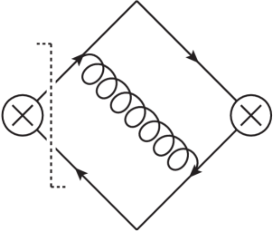
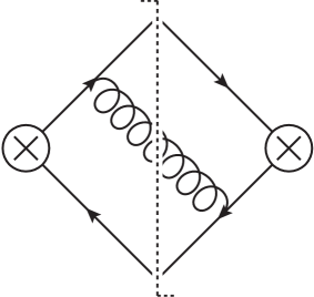
Figure 1: Both the virtual contribution (left) and real contribution (right) to the $\alpha_{s}$ cross section can be drawn as cut diagrams with the same topology.

At order $\alpha_{s}$, the virtual contribution to a cross section contributes by interfering with the tree-level graph. This interference can be drawn as a cut diagram (Fig. 1, left), which is nearly identical to the real emission graph (Fig. 1, right). By moving the cut, the propagator in the virtual graph is replaced by an on-shell condition. That is,

$$d\sigma_{V}\propto-\mathcal{P}_{ab}^{1}\frac{d^{4}p_{1}}{(2\pi)^{4}}\frac{i}{p^{2}+i\varepsilon},\quad\quad d\sigma_{R}\propto\mathcal{P}_{ab}^{1}\frac{d^{4}p_{1}}{(2\pi)^{3}}\theta(\omega_{1})\delta(p_{1}^{2}),\hskip 10.00002pt$$ (24)

with the minus sign in the virtual contribution arising since the cut is on one side of the emissions only. To relate the two contributions, we can cut the propagator ourselves through the identity

$$\frac{i}{p^{2}+i\varepsilon}=\text{PV}\left\{\dfrac{i}{p^{2}}\right\}+\pi\delta(p^{2})\theta(p_{0})+\pi\delta(p^{2})\theta(-p_{0})$$ (25)

Since all the components of $p_{1}^{\mu}$ are very small, by the SEO assumption, the virtual gluon is nearly on shell. In this limit, the principal value contribution vanishes. More generally, since the principle value is not IR-sensitive, it can contribute only a finite part to the cross section, not a large logarithm. The $\delta(p^{2})$ terms in Eq. (25) have support for either $p_{0}>0$ or $p_{0}<0$, each of which give the same contribution. Thus we can replace $\frac{i}{p^{2}+i\varepsilon}\rightarrow 2\pi\theta(p_{0})\delta(p^{2})$ in the virtual contribution showing it to have the same form as the real emission, up to a sign.

Another way to understand the connection between real and virtual is to use that in a sufficiently inclusive cross section, the large logarithm from real emission must be exactly canceled by virtual corrections. Thus we should be able to represent the virtual contributions as integrals over momenta of exactly the same form as the real emissions. For example, at 1 loop, we would have

$$d\sigma_{V}=-d\sigma_{R}\propto-Ng^{2}\frac{1}{\omega_{1}^{2}}\mathcal{P}_{ab}^{1}$$ (26)

Let us abbreviate this with

$${\mathcal{W}}_{R}=\mathcal{P}_{ab}^{1},\hskip 10.00002pt{\mathcal{W}}_{V}=-{\mathcal{W}}_{R}$$ (27)

For an observable which is not totally inclusive, like the hemisphere mass, there will be an incomplete cancellation between the real and virtual corrections, leaving a large logarithm.

For more general notation, let us write ${\mathcal{W}}_{RV\cdots R}$ to indicate that the hardest gluon, $1$, is real, the second hardest, 2, is virtual and so on down to the softest, $m$, which in this case is real. Thus, for example, at $\alpha_{s}^{2}$, the differential cross section can be written as, using Eq. (16)

$$\frac{1}{\sigma_{0}}d\sigma_{m}=\hskip 14.22636pt\bar{\alpha}\frac{d\omega_{1}}{\omega_{1}}\frac{d\Omega_{1}}{4\pi}\left({\mathcal{W}}_{R}+{\mathcal{W}}_{V}\right)\\ +\frac{\bar{\alpha}^{2}}{2!}\frac{d\omega_{1}}{\omega_{1}}\frac{d\Omega_{1}}{4\pi}\frac{d\omega_{2}}{\omega_{2}}\frac{d\Omega_{2}}{4\pi}\left({\mathcal{W}}_{RR}+{\mathcal{W}}_{RV}+{\mathcal{W}}_{VR}+{\mathcal{W}}_{VV}\right)\\ +\frac{\bar{\alpha}^{3}}{3!}\frac{d\omega_{1}}{\omega_{1}}\frac{d\Omega_{1}}{4\pi}\frac{d\omega_{2}}{\omega_{2}}\frac{d\Omega_{2}}{4\pi}\frac{d\omega_{3}}{\omega_{3}}\frac{d\Omega_{3}}{4\pi}\left({\mathcal{W}}_{RRR}+{\mathcal{W}}_{RRV}+\cdots\right)$$ (28)

For two emissions, the gluons can be either real or virtual. If both are real, we get the expression in Eq. (21):

$${\mathcal{W}}_{RR}=\mathcal{P}_{ab}^{12}=\mathcal{P}_{ab}^{1}\left[\mathcal{P}_{a1}^{2}+\mathcal{P}_{1b}^{2}\right]$$ (29)

This holds for either $\omega_{1}\gg\omega_{2}$ or $\omega_{2}\gg\omega_{1}$. If the harder gluon is real and the softer gluon is virtual, the real emission establishes the $(a1)$ and $(1b)$ dipoles, which then each contribute a virtual contribution. So we have

$${\mathcal{W}}_{RV}=-\mathcal{P}_{ab}^{1}\left[\mathcal{P}_{a1}^{2}+\mathcal{P}_{1b}^{2}\right]$$ (30)

On the other hand, if the harder gluon ($1$) is virtual, then the virtual graph does not produce any new dipoles. So we get $-\mathcal{P}_{ab}^{1}$ for the first emission, but have only the original $ab$ dipole to produce subsequent emissions. This dipole then produces the real emission and we have

$${\mathcal{W}}_{VR}=-\mathcal{P}_{ab}^{1}\mathcal{P}_{ab}^{2}$$ (31)

If both the harder and softer gluon are virtual, then the $ab$ dipole produces both, each get a minus sign, and we find

$${\mathcal{W}}_{VV}=\mathcal{P}_{ab}^{1}\mathcal{P}_{ab}^{2}$$ (32)

Thus there are 2 independent integrands

$$B_{1} =\mathcal{P}_{ab}^{12}={\mathcal{W}}_{RR}=-{\mathcal{W}}_{RV}$$ (33)

$$B_{2} =\mathcal{P}_{ab}^{1}\mathcal{P}_{ab}^{2}={\mathcal{W}}_{VV}=-{\mathcal{W}}_{VR}$$ (34)

At order $\alpha_{s}^{3}$, we construct the real and virtual integrands in the same iterative way. For example, the contribution with all gluons virtual comes from 3 uncorrelated emissions from the $(ab)$ dipole, each with a minus sign:

$${\mathcal{W}}_{VVV}=-{\mathcal{W}}_{ab}^{1}{\mathcal{W}}_{ab}^{2}{\mathcal{W}}_{ab}^{3}$$ (35)

When the hardest gluon is real and the second is virtual, we get $\mathcal{-P}_{ab}^{12}$ as above. Since the second gluon is virtual, it does not produce a new dipole, so the 3rd emission comes from the $\left(a1\right)$ and $\left(2b\right)$ dipoles only. Thus we find

$${\mathcal{W}}_{RVR}=-{\mathcal{W}}_{RVV}=-\mathcal{P}_{ab}^{12}\left(\mathcal{P}_{a1}^{3}+\mathcal{P}_{b1}^{3}\right)$$ (36)

In total at order $\alpha_{s}^{3}$, there are 4 independent integrands:

$$C_{1} =\mathcal{P}_{ab}^{123}={\mathcal{W}}_{RRR}=-{\mathcal{W}}_{RRV}$$ (37)

$$C_{2} =\mathcal{P}_{ab}^{12}\left(\mathcal{P}_{a1}^{3}+\mathcal{P}_{b1}^{3}\right)={\mathcal{W}}_{RVV}=-{\mathcal{W}}_{RVR}$$ (38)

$$C_{3} =\mathcal{P}_{ab}^{1}\mathcal{P}_{ab}^{23}=-{\mathcal{W}}_{VRR}={\mathcal{W}}_{VRV}$$ (39)

$$C_{4} =\mathcal{P}_{ab}^{1}\mathcal{P}_{ab}^{2}\mathcal{P}_{ab}^{3}={\mathcal{W}}_{VVR}=-{\mathcal{W}}_{VVV}$$ (40)

Summing all eight contributions gives zero, as expected since there can be no large logarithms in an inclusive cross section. The procedure for constructing the real and virtual contributions to $\left|\mathcal{M}\right|^{2}$ to arbitrary order should now be clear by generalizing these examples.

4 The non-global hemisphere mass integral

The procedure defined in the previous sections provide the real and virtual contributions to $|\mathcal{M}|^{2}$ in the SEO approximation. To construct an observable, we have to integrate these matrix elements against a measurement function. Since virtual gluons are never measured, this function is only sensitive to the gluons which are real. In this section, we work out the integrand at up to 3 loops and outline the procedure for higher loops. Above 3 loops, we find it simpler to extract the NGL integrand using the BMS equation, as explained in the next section.

To avoid dealing with distributions, we work with the cumulant right-hemisphere mass defined as $\rho=\frac{M_{R}}{Q}$. We then have

$$S(\rho)=\frac{1}{\sigma_{0}}\int_{0}^{Q}dm_{L}\int_{0}^{\rho Q}dm_{R}\frac{d^{2}\sigma}{dm_{L}dm_{R}}$$ (41)

We can therefore write the cross section as the integral of the matrix-element squared times a measurement function

$$S(\rho)=\int d\Phi_{m}\left|\mathcal{M}_{ab}^{1\cdots m}\right|^{2}u(\{p_{i}\})$$ (42)

where the measurement function for the hemisphere mass cumulant at leading power is

$$u(\{p_{i}\})=\Theta\Big{(}\rho Q-\sum_{i}2(p_{i}\cdot n)\theta_{R}(p_{i})\Big{)}$$ (43)

Working in a frame where the jet are back-to-back in the $n^{\mu}=(1,\vec{n})$ and $\overline{n}^{\mu}=(1,-\vec{n})$ directions, the right-hemisphere projector is $\theta_{R}(p)\equiv\theta(\vec{p}\cdot\vec{n})$. Similarly, the left-hemisphere projector is $\theta_{L}(p)\equiv\theta(-\vec{p}\cdot\vec{n})=1-\theta_{R}(p)$. Since only the hardest gluon in the hemisphere will contribute, we can equally well use

$$u(\{p_{i}\})=\prod_{p_{i}}u(p_{i})$$ (44)

where

$$u\left(p\right)=\Theta(\rho Q-2p\cdot n)\theta_{R}(p)+\theta_{L}(p)$$ (45)

That we can treat the emissions independently greatly simplifies the calculation.

For one emission, we can write the cumulant as

$$S^{(1)}(\rho)=\bar{\alpha}\int{\mathcal{W}}_{R}u(p_{1})+\bar{\alpha}\int{\mathcal{W}}_{V},$$ (46)

where no phase space constraint is imposed on the virtual gluon, as the measurement operator does not act on the virtual gluons. Let us write more suggestively,

$$u(p_{1})=\Theta(\rho Q-2p_{1}\cdot n)\theta_{R}(p_{1})=1_{R}\theta_{1<\rho}+1_{L}$$ (47)

$1_{R}$ means that gluon 1 goes to the right and $\theta_{1<\rho}$ means that gluon 1’s contribution to the hemisphere mass is not larger than $\rho$. Using Eq. (27) the $\mathcal{O}(\alpha_{s})$ result is then

$$S^{(1)}(\rho)=\bar{\alpha}\int\mathcal{P}_{ab}^{1}(1_{R}\theta_{1<\rho}+1_{L}-1)=-\bar{\alpha}\int\mathcal{P}_{ab}^{1}1_{R}\theta_{\rho<1}$$ (48)

This is the global logarithm. To all orders, the global logarithm is given by the exponentiation of this term.

For two emissions, we have

$$S^{\left(2\right)}\left(\rho\right)=\bar{\alpha}^{2}\int_{E_{1}>E_{2}}\left(1_{R}\theta_{1<\rho}+1_{L}\right)\left(2_{R}\theta_{2<\rho}+2_{L}\right){\mathcal{W}}_{RR}+\bar{\alpha}^{2}\int_{E_{1}>E_{2}}\left(1_{R}\theta_{1<\rho}+1_{L}\right){\mathcal{W}}_{RV}\\ +\bar{\alpha}^{2}\int_{E_{1}>E_{2}}\left(2_{R}\theta_{2<\rho}+2_{L}\right){\mathcal{W}}_{VR}+\bar{\alpha}^{2}\int_{E_{1}>E_{2}}{\mathcal{W}}_{VV}$$ (49)

Our notation is defined so that gluon 1 is much harder than gluon 2. Therefore $\theta_{\rho<1}\theta_{\rho<2}=\theta_{\rho<2}$. For the same reason, we can drop the symmetry factor $1/2!$, since only one energy ordering is picked out for the phase space integral. We can then write $S^{\left(2\right)}(\rho)$ suggestively as

$$S^{(2)}(\rho)=\bar{\alpha}^{2}\int_{E_{1}>E_{2}}1_{R}2_{R}\theta_{\rho<1}\theta_{\rho<2}\left(\mathcal{P}_{ab}^{1}\mathcal{P}_{ab}^{2}\right)-\bar{\alpha}^{2}\int_{E_{1}>E_{2}}1_{L}2_{R}\theta_{\rho<2}\left(\mathcal{P}_{ab}^{12}-\mathcal{P}_{ab}^{1}\mathcal{P}_{ab}^{2}\right)$$ (50)

The first term here is the global contribution with both gluons going right but uncorrelated.  If we average the first integral over the same thing with $E_{2}>E_{1}$, we can drop the energy ordering and have simply

$$\bar{\alpha}^{2}\int_{E_{1}>E_{2}}1_{R}2_{R}\theta_{\rho<2}\left(\mathcal{P}_{ab}^{1}\mathcal{P}_{ab}^{2}\right)=\frac{\bar{\alpha}^{2}}{2}\int 1_{R}2_{R}\theta_{\rho<1}\theta_{\rho<2}\mathcal{P}_{ab}^{1}\mathcal{P}_{ab}^{2}=\frac{1}{2}\left[S^{\left(1\right)}\left(\rho\right)\right]^{2},$$ (51)

which agrees with the second-order expansion of $\exp\left(S^{\left(1\right)}\left(\rho\right)\right)$. The second term in Eq. (50) when integrated gives the leading non-global logarithm. Explicitly,

$$S^{(2)}_{\text{NG}}= -\bar{\alpha}^{2}\int_{E_{1}>E_{2}}1_{L}2_{R}\theta_{\rho<2}\left(\mathcal{P}_{ab}^{12}-{\mathcal{W}}_{ab}^{1}{\mathcal{W}}_{ab}^{2}\right)$$

$$= -\bar{\alpha}^{2}\int_{0}^{Q}\frac{d\omega_{2}}{\omega_{2}}\int_{\text{right}}\frac{d\Omega_{2}}{4\pi}\int_{\omega_{2}}^{Q}\frac{d\omega_{1}}{\omega_{1}}\int_{\text{left}}\frac{d\Omega_{1}}{4\pi}\theta\left(\omega_{2}-\frac{\rho Q}{2(n2)}\right)$$

$$\hskip 85.35826pt\times\left[\frac{(n\overline{n})}{(n1)(12)(2\overline{n})}+\frac{(n\overline{n})}{(n2)(21)(1\overline{n})}-\frac{(n\overline{n})}{(n1)(1\overline{n})}\frac{(n\overline{n})}{(n2)(2\overline{n})}\right]$$

$$= -\bar{\alpha}^{2}\frac{\pi^{2}}{24}\ln^{2}\rho+\text{less singular terms}$$ (52)

This integrand is exactly that given by Eq. (8) of Ref. [37].

A simplifying observation is that because the non-global integral has no collinear singularities, we can replace the $\theta$ function on hemisphere mass with a simpler one on energy: $\theta\left(\omega_{2}-\frac{\rho Q}{2(n2)}\right)\rightarrow\theta(\omega_{2}-\rho)$. The difference produces only subleading terms. This is not allowed in the global logarithmic terms because unregulated collinear divergences would arise, but is allowed for non-global ones.

The first new result here is the 3-loop integrand. Following the same procedure outlined above, we find

$$S^{\left(3\right)}\left(\rho\right)=\bar{\alpha}^{3}\int_{E_{1}>E_{2}>E_{3}}1_{R}2_{R}3_{R}\theta_{\rho<3}\left(-C_{4}\right)+\bar{\alpha}^{3}\int_{E_{1}>E_{2}>E_{3}}1_{R}2_{L}3_{R}\theta_{\rho<3}\left(C_{3}-C_{4}\right)\\ +\bar{\alpha}^{3}\int_{E_{1}>E_{2}>E_{3}}1_{L}2_{R}3_{R}\theta_{\rho<3}\left(C_{2}-C_{4}\right)+\bar{\alpha}^{3}\int_{E_{1}>E_{2}>E_{3}}1_{L}2_{L}3_{R}\theta_{\rho<3}\left(-C_{1}+C_{2}+C_{3}-C_{4}\right)$$ (53)

with $C_{1}$, $C_{2}$, $C_{3}$ and $C_{4}$ given in Eqs. (37). To find the 3-loop NGLs, we have to remove the global logarithms. To find the purely 3-loop contribution, we should also remove the exponentiation of all the previous terms. Writing the cumulant in an exponentiated form,

$$S=\exp\left(S^{\left(1\right)}+S_{\text{NG}}^{(2)}+S_{\text{NG}}^{\left(3\right)}+\cdots\right),$$ (54)

we find

$$S_{\text{NG}}^{\left(3\right)}=\bar{\alpha}^{3}\int_{E_{1}>E_{2}>E_{3}}1_{L}2_{R}3_{R}\theta_{\rho<3}\left(\overline{C_{2}-C_{4}}\right)+\bar{\alpha}^{3}\int_{E_{1}>E_{2}>E_{3}}1_{L}2_{L}3_{R}\theta_{\rho<3}\left(-C_{1}+C_{2}+C_{3}-C_{4}\right)$$ (55)

where

$$\overline{C_{2}-C_{4}}=\mathcal{P}_{ab}^{12}\left(\mathcal{P}_{a1}^{3}+\mathcal{P}_{1b}^{3}\right)-\mathcal{P}_{ab}^{1}\mathcal{P}_{ab}^{2}\mathcal{P}_{ab}^{3}-\mathcal{P}_{ab}^{2}\left[\mathcal{P}_{ab}^{13}-\mathcal{P}_{ab}^{1}\mathcal{P}_{ab}^{3}\right]-\mathcal{P}_{ab}^{3}\left[\mathcal{P}_{ab}^{12}-\mathcal{P}_{ab}^{1}\mathcal{P}_{ab}^{2}\right]$$ (56)

Both terms in Eq. (55) are free of collinear singularities.

Note that at 3 loops, it is not true that only the softest gluon goes to the right. The $2_{R}$ in Eq. (55) indicates that a contribution also comes from the middle gluon going to the right. However, this is somewhat of an illusion. Since all the integrands which give $\pm C_{2}$ or $\pm C_{4}$ have the second gluon virtual, all the $2_{R}$ terms in the first term in Eq. (55) correspond to virtual emissions. Thus, while there is a $2_{R}$ contribution, a real gluon which is not the softest never actually goes into the right hemisphere.

While we could proceed to evaluate $S_{\text{NG}}^{\left(3\right)}$ at this point, it is somewhat simpler first to reproduce $S_{\text{NG}}^{\left(3\right)}$ from a recursive formula (the BMS equation). This will simplify the calculation at 3 loops and beyond, as we will now see.

5 BMS equation

The BMS equation [40] is an integro-differential equation whose solution gives the leading NGLs (those of the form $(\bar{\alpha}\ln\rho)^{n}$, for $n>1$) at large $N_{c}$. The derivation of the BMS equation for the hemisphere mass proceeds identically to the derivation for the out-of-jet energy given in Ref. [40]. We have nothing profound to add to the derivation, so we simply present the result. For the hemisphere case, the BMS equation becomes

$$\partial_{L}G_{ab}(L)=\int\frac{d\Omega_{j}}{4\pi}{\mathcal{W}}_{ab}^{j}\left[\theta_{L}(j)G_{aj}(L)G_{jb}(L)-G_{ab}(L)\right],$$ (57)

Here, ${\mathcal{W}}_{ab}^{j}$ is the dipole radiator, from Eq. (13):

$${\mathcal{W}}_{ab}^{j}=\frac{(ab)}{(aj)(jb)}$$ (58)

with $(ab)=\frac{a\cdot b}{\omega_{a}\omega_{b}}$ and $\theta_{L}(j)$ restricts the angular integral to being over the left-hemisphere. Recall that our convention is such that $n^{\mu}$ points to the right hemisphere and $\overline{n}^{\mu}$ to the left hemisphere and that

$$\cos\theta_{n}=-1,\qquad\cos\theta_{\overline{n}}=1$$ (59)

The solution to the BMS equation are a set of functions $G_{ab}(L)$ indexed by lightlike directions $a^{\mu}$ and $b^{\mu}$ (equivalently angles $\Omega_{a}$ and $\Omega_{b}$ on the 2-sphere). These functions, when evaluated at

$$L={\widehat{L}}\equiv N_{c}\frac{\alpha_{s}}{\pi}\ln\frac{1}{\rho},$$ (60)

give all the single (global and non-global) logarithms of the hemisphere mass from a color dipole in $a^{\mu}$ and $b^{\mu}$ directions. In particular, the hemisphere mass NGLs are in $G_{n\overline{n}}({\widehat{L}})$. There are additional single logarithms coming from the 1-loop running of $\alpha_{s}$. These can be easily included [37], so we simply ignore them for simplicity.

To extract just the NGLs, following BMS we write

$$G_{ab}(L)=g_{ab}(L)\exp\left(-{L}\int_{\text{right}}\frac{d\Omega_{j}}{4\pi}{\mathcal{W}}_{ab}^{j}\right),$$ (61)

which leads to

$$\partial_{L}g_{ab}(L)=\int_{\text{left}}\frac{d\Omega_{j}}{4\pi}{\mathcal{W}}_{ab}^{j}\left[U_{abj}(L)g_{aj}(L)g_{jb}(L)-g_{ab}(L)\right],$$ (62)

with

$$U_{abj}(L)=\exp\left[{L}\int_{\text{right}}\frac{d\Omega_{1}}{4\pi}\left({\mathcal{W}}_{ab}^{1}-{\mathcal{W}}_{aj}^{1}-{\mathcal{W}}_{jb}^{1}\right)\right].$$ (63)

The boundary conditions on the BMS equation are that $g_{ab}(0)=G_{ab}(0)=1$ for all $a$ and $b$. Importantly, this boundary condition respects any symmetry acting on $a$ and $b$.

Before exploring the perturbative solution to the BMS equation, let us quickly consider the symmetries of $g_{ab}({L})$ for different $a$ and $b$. The directions $a$ and $b$ can be arbitrary angles $(\theta_{a},\phi_{a})$ and $(\theta_{b},\phi_{b})$ on 2-sphere. There is an obvious cylindrical symmetry with respect to the hemisphere axis which makes $g_{ab}({L})$ only depend on $\phi_{b}-\phi_{a}$. Thus one would think there are three degrees of freedom in $g_{ab}(L)$. Remarkably however, the BMS equation contains a hidden ${\rm PSL}(2,\mathbb{R})$ symmetry, and there is actually only one degree of freedom in $g_{ab}(L)$: the geodesic distance between $a$ and $b$ on the Poincaré disk. We explain this symmetry in Section 6.2.

5.1 Perturbative check

First, let us check that the perturbative expansion of the BMS equation for $g_{n\overline{n}}$ reproduces the integrands at 2 and 3 loops that were derived in Sections 3 and 4 by summing virtual and real corrections using the strong-energy-ordered approximation.

To work perturbatively we write, $g_{ab}(L)=\sum_{m=0}^{\infty}g_{ab}^{(m)}$ with $g_{ab}^{(m)}$ proportional to $L^{m}$, and similarly for $U_{abj}$. Substituting $g_{ab}^{(0)}=g_{ab}(0)=1$ and $U_{abj}^{(0)}=1$, right-hand side of Eq. (62) vanishes. Integrating Eq. (62) we then find that there is no $\mathcal{O}(L)$ term in $g_{ab}(L)$, consistent with the leading non-global logarithm starting at 2 loops.

At order $L$, labeling the radiated gluon $2$ for convenience, we have

$$U_{abj}^{(1)}(L)={L}\int_{\text{right}}\frac{d\Omega_{2}}{4\pi}\left({\mathcal{W}}_{ab}^{2}-{\mathcal{W}}_{aj}^{2}-{\mathcal{W}}_{jb}^{2}\right)$$ (64)

and so

$$\partial_{L}g_{ab}^{\left(2\right)}\left(L\right)=-{L}\int_{\text{left}}\frac{d\Omega_{1}}{4\pi}{\mathcal{W}}_{ab}^{1}\left[\int_{\text{right}}\frac{d\Omega_{2}}{4\pi}\left({\mathcal{W}}_{aj}^{2}-{\mathcal{W}}_{jb}^{2}-{\mathcal{W}}_{ab}^{2}\right)\right],$$ (65)

giving

$$g_{ab}^{\left(2\right)}\left(L\right)=-\frac{1}{2}{L}^{2}\int_{\Omega}1_{L}2_{R}\left(\mathcal{P}_{ab}^{12}-{\mathcal{W}}_{ab}^{1}{\mathcal{W}}_{ab}^{22}\right),$$ (66)

where $\int_{\Omega}1_{L}2_{R}=\int_{\text{left}}\frac{d\Omega_{1}}{4\pi}\int_{\text{right}}\frac{d\Omega_{2}}{4\pi}$. Eq. (66) agrees exactly with Eq. (52).

For $g_{ab}^{\left(3\right)}$ we need $U_{abj}^{\left(2\right)}$ and $g_{ab}^{\left(2\right)}$. So,

$$\partial_{L}g_{ab}^{\left(3\right)}\left(L\right)=\frac{1}{2}{L}^{2}\int_{\Omega}1_{L}2_{R}3_{R}{\mathcal{W}}_{ab}^{1}\left({\mathcal{W}}_{a1}^{2}+{\mathcal{W}}_{1b}^{2}-{\mathcal{W}}_{ab}^{2}\right)\left({\mathcal{W}}_{a1}^{3}+{\mathcal{W}}_{1b}^{3}-{\mathcal{W}}_{ab}^{3}\right)\\ -\frac{1}{2}{L}^{2}\int_{\Omega}1_{L}2_{L}3_{R}{\mathcal{W}}^{1}_{ab}\left[\left({\mathcal{P}}_{a1}^{23}-{\mathcal{W}}_{a1}^{2}{\mathcal{W}}_{a1}^{3}\right)+\left({\mathcal{P}}_{1b}^{23}-{\mathcal{W}}_{1b}^{2}{\mathcal{W}}_{1b}^{3}\right)-\left({\mathcal{P}}_{ab}^{23}-{\mathcal{W}}_{ab}^{2}{\mathcal{W}}_{ab}^{3}\right)\right]$$ (67)

Integrating gives

$$g_{ab}^{\left(3\right)}\left(L\right)=\frac{1}{3!}{L}^{3}\int_{\Omega}1_{L}2_{R}3_{R}{\mathcal{W}}_{ab}^{1}\left({\mathcal{W}}_{a1}^{2}+{\mathcal{W}}_{1b}^{2}-{\mathcal{W}}_{ab}^{2}\right)\left({\mathcal{W}}_{a1}^{3}+{\mathcal{W}}_{1b}^{3}-{\mathcal{W}}_{ab}^{3}\right)\\ -\frac{1}{3!}{L}^{3}\int_{\Omega}1_{L}2_{L}3_{R}{\mathcal{W}}^{1}_{ab}\left[\left({\mathcal{P}}_{a1}^{23}-{\mathcal{W}}_{a1}^{2}{\mathcal{W}}_{a1}^{3}\right)+\left({\mathcal{P}}_{1b}^{23}-{\mathcal{W}}_{1b}^{2}{\mathcal{W}}_{1b}^{3}\right)-\left({\mathcal{P}}_{ab}^{23}-{\mathcal{W}}_{ab}^{2}{\mathcal{W}}_{ab}^{3}\right)\right]$$ (68)

which agrees with Eq. (55).

It quickly becomes clear that this is a much simpler way to generate the integrand than following the real/virtual emission rules as in Sections 3 and 4. More importantly, the BMS equation clarifies the symmetries of $g_{ab}$ which are not at all apparent working order by order using the SEO approximation, as we will soon see.

6 Simplifying and solving the BMS equation

Before trying to iterate and integrate the BMS equation, it will be helpful to calculate $U_{abj}$ in Eq. (63) exactly. This will produce a form of the measure in the BMS equation which manifests the ${\rm PSL}(2,\mathbb{R})$ symmetry.

6.1 Exact solution for $U_{abj}$

Note that from Eq. (62) the $j$ emission is always in the left hemisphere. Thus the only relevant direction in the right hemisphere is the hemisphere axis $n$. Thus, for the hemisphere NGLs, we only need $U_{anj}$ and $U_{abj}$ with $ab$ and $j$ going left. The dipole radiator ${\mathcal{W}}_{ab}^{j}=\frac{(ab)}{(aj)(jb)}$ depends on the round bracket from Eq. (12) which can be expanded as

$$(ab)=1-\cos\theta_{ab}=1-\cos\theta_{a}\cos\theta_{b}-\cos(\phi_{a}-\phi_{b})\sin\theta_{a}\sin\theta_{b}$$ (69)

It is helpful also to define a square bracket as the round bracket with one of the vectors reflected to the opposite hemisphere:

$$[ab]\equiv(\bar{a}b)=1+\cos\theta_{a}\cos\theta_{b}-\cos(\phi_{a}-\phi_{b})\sin\theta_{a}\sin\theta_{b}$$ (70)

Now, if $a$ and $b$ are both left, but the emission goes right, then there are no collinear singularities in the angular integral and the dipole radiator can be easily integrated

$$\int_{\text{right}}\frac{d\Omega_{1}}{4\pi}{\mathcal{W}}_{ab}^{1}=\frac{1}{2}\ln\frac{\left[ab\right]}{2\cos\theta_{a}\cos\theta_{b}}$$ (71)

Adding three of these and exponentiating with Eq. (63) leads to

$$U_{abj}(L)=2^{{L}/2}\cos^{L}\theta_{j}\left\{\frac{[ab]}{[aj][jb]}\right\}^{{L}/2}$$ (72)

Therefore, Eq. (62) reduces to

$$\partial_{L}g_{ab}(L)=\frac{1}{4\pi}\int_{0}^{1}d\cos\theta_{j}\int_{0}^{2\pi}d\phi_{j}\frac{(ab)}{(aj)(jb)}\\ \times\left[2^{{L}/2}\cos^{L}\theta_{j}\left\{\frac{[ab]}{[aj][jb]}\right\}^{{L}/2}g_{aj}(L)g_{jb}(L)-g_{ab}(L)\right]\quad(a,b~{}~{}\text{both left})$$ (73)

Note that when $a$ and $b$ are both left, to all orders the BMS equation only involves directions in the left hemisphere.

When one of the directions is $n$, which is in the right hemisphere, then the integral in Eq. (71) has a collinear divergences, but $U_{abj}$ is still finite. We find

$$U_{anj}\left(L\right)=2^{{L}/2}\cos^{L}\theta_{j}\left\{\frac{\left(an\right)}{[aj](jn)}\right\}^{{L}/2},$$ (74)

and so Eq. (62) becomes

$$\partial_{L}g_{an}(L)=\frac{1}{4\pi}\int_{0}^{1}d\cos\theta_{j}\int_{0}^{2\pi}d\phi_{j}\frac{(an)}{(aj)(jn)}\\ \times\left[2^{{L}/2}\cos^{L}\theta_{j}\left\{\frac{(an)}{[aj](jn)}\right\}^{{L}/2}g_{aj}(L)g_{jn}(L)-g_{an}(L)\right]\quad(a~{}\text{left})$$ (75)

6.2 Symmetries of the BMS equation

Having evaluated $U_{abj}$ exactly, the BMS equation, as in Eq. (73) now depends only on the $g_{ab}(L)$ functions and an explicit integration measure. In this form it is simpler to explore its symmetries. In the following discussion, we will first concentrate on the BMS equation when both $a$ and $b$ are in the left hemisphere (as of course is the emission $j$). The case when $b$ is in the left hemisphere is similar, but the symmetry is less obvious. We present both results in the end.

It has been observed that the BMS equation is formally similar to the BK equation [48, 49], a non-linear integro-differential equation describing gluon saturation effects. The BK equation enjoys a conformal symmetry ${\rm PSL}(2,\mathbb{C})$ in its integral measure (see, e.g., [58]), which is violated by initial conditions. It is therefore natural to look for a similar symmetry in the BMS equation. Indeed, it has been observed that the integration measure of the BMS equation does indeed respect ${\rm PSL}(2,\mathbb{C})$ [59, 60]. Moreover, unlike for the BK equation, this symmetry is not broken by the initial condition of the BMS equation. However, it is broken by the restriction on the integration region. As we will now explain, for the hemisphere mass case, the restriction that radiation goes into the left hemisphere breaks the symmetry from ${\rm PSL}(2,\mathbb{C})$ to ${\rm PSL}(2,\mathbb{R})$.

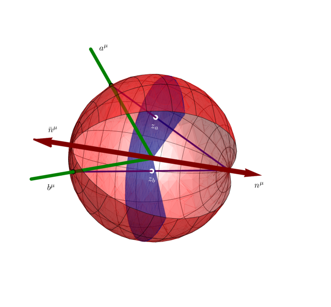
Figure 2: A stereographic projection of the jet directions onto the Poincaré disk reveals the ${\rm PSL}(2,\mathbb{R})$ symmetry of the BMS equation.

To reveal the symmetry of the BMS equation, it’s useful to consider a change of variables by stereographic projection  [59, 60],

$$z=\frac{\sin\theta}{1+\cos\theta}e^{i\phi}$$ (76)

This projection is shown in Fig. 2. Under the stereographic projection transformation, the full angle space $(\theta,\phi)$ coordinate is mapped to the full complex plane, while the left hemisphere, $\cos\theta>0$, is mapped to the unit disk.

In terms of $z$, the angle from the hemisphere axis is

$$\cos\theta=\frac{1-|z|^{2}}{1+|z|^{2}}$$ (77)

and the angular measure on the sphere turns into

$$d\Omega=d\cos\theta d\phi=\frac{4dz\,d\bar{z}}{(1+|z|^{2})^{2}}$$ (78)

Also, the round and square bracket inner products, in Eqs. (69) and (70) become

$$(ij)=2\frac{|z_{i}-z_{j}|^{2}}{(1+|z_{i}|^{2})(1+|z_{j}|^{2})},\qquad[ij]=(ij)+2\left(\frac{1-|z_{i}|^{2}|}{1+|z_{i}|^{2}}\right)\left(\frac{1-|z_{j}|^{2}|}{1+|z_{j}|^{2}}\right),$$ (79)

and the radiator times the measure becomes

$$d\Omega_{j}\,{\mathcal{W}}_{ab}^{j}=d\Omega\frac{(ab)}{(aj)(jb)}=2dzd\bar{z}\frac{|z_{a}-z_{b}|^{2}}{|z_{a}-z_{j}|^{2}|z_{j}-z_{b}|^{2}}$$ (80)

Recall that the angle and square brackets come from Lorentzian inner products of normalized 4-vectors on the unit sphere. Although the sphere is Euclidean, these inner products are naturally hyperbolic. Indeed, the inner products are reminiscent of the hyperbolic distance measure on the Poincaré disk, defined as

$${\color[rgb]{0.7,0.0,0.0}\langle}{ij}{\color[rgb]{0.7,0.0,0.0}\rangle}=\frac{|z_{i}-z_{j}|^{2}}{(1-|z_{i}|^{2})(1-|z_{j}|^{2})}=\frac{(ij)}{2\cos\theta_{i}\cos\theta_{j}}$$ (81)

It then follows that

$$(ij) =2\cos\theta_{i}\cos\theta_{j}{\color[rgb]{0.7,0.0,0.0}\langle}{ij}{\color[rgb]{0.7,0.0,0.0}\rangle}=2\left(\frac{1-|z_{i}|^{2}}{1+|z_{i}|^{2}}\right)\left(\frac{1-|z_{j}|^{2}}{1+|z_{j}|^{2}}\right){\color[rgb]{0.7,0.0,0.0}\langle}{ij}{\color[rgb]{0.7,0.0,0.0}\rangle}$$ (82)

$$[ij] =2\cos\theta_{i}\cos\theta_{j}\Big{(}1+{\color[rgb]{0.7,0.0,0.0}\langle}{ij}{\color[rgb]{0.7,0.0,0.0}\rangle}\Big{)}=2\left(\frac{1-|z_{i}|^{2}}{1+|z_{i}|^{2}}\right)\left(\frac{1-|z_{j}|^{2}}{1+|z_{j}|^{2}}\right)\Big{(}1+{\color[rgb]{0.7,0.0,0.0}\langle}{ij}{\color[rgb]{0.7,0.0,0.0}\rangle}\Big{)}$$ (83)

Plugging these equations into the BMS equation for left-hemisphere NGLs, Eq. (73), we obtain

$$\partial_{L}g_{ab}(L)= \int_{|z|<1}\frac{dz_{j}\,d\bar{z}_{j}}{2\pi}\frac{|z_{a}-z_{b}|^{2}}{|z_{a}-z_{j}|^{2}|z_{j}-z_{b}|^{2}}$$

$$\times\left\{\left[\frac{1+{\color[rgb]{0.7,0.0,0.0}\langle}{ab}{\color[rgb]{0.7,0.0,0.0}\rangle}}{(1+{\color[rgb]{0.7,0.0,0.0}\langle}{aj}{\color[rgb]{0.7,0.0,0.0}\rangle})(1+{\color[rgb]{0.7,0.0,0.0}\langle}{jb}{\color[rgb]{0.7,0.0,0.0}\rangle})}\right]^{{L}/2}g_{aj}(L)g_{jb}(L)-g_{ab}(L)\right\}.$$ (84)

In this form, the symmetry of the BMS equation under ${\rm PSL}(2,\mathbb{R})$ is easiest to verify. First, we note that the radiator itself

$$d\Omega_{j}\,{\mathcal{W}}_{ab}^{j}=dz_{j}\,d\bar{z}_{j}\frac{|z_{a}-z_{b}|^{2}}{|z_{a}-z_{j}|^{2}|z_{j}-z_{b}|^{2}},$$ (85)

or more simply its holomorphic half,

$$dz_{j}\frac{(z_{a}-z_{b})}{(z_{a}-z_{j})(z_{j}-z_{b})},$$ (86)

is invariant under (i) $z\to z+\lambda$ ($\lambda\in\mathbb{C}$); (ii) $z\to\lambda z$, ($\lambda\neq 0$) and (iii) $z\to-1/z$. These symmetries generate fractional linear transformations of the form

$$z\to\frac{\alpha z+\beta}{\gamma z+\delta}=\frac{\alpha}{\gamma}+\frac{\beta-\frac{\alpha\delta}{\gamma}}{\gamma z+\delta},\qquad\alpha\delta-\beta\gamma=1,\qquad{\rm and}\;\;\alpha,\beta,\gamma,\delta\in\mathbb{C}.$$ (87)

The matrices $\begin{pmatrix}\alpha&\beta\\ \gamma&\delta\end{pmatrix}$ are elements of the Möbius group ${\rm PSL}(2,\mathbb{C})=\mathrm{SL}(2,\mathbb{C})/(\pm I)$, where $I$ is the unit matrix. One way to understand why the radiator is invariant under Möbius transformations, is to recall that these transformations can be derived by projecting the disk onto the unit sphere, rotating the sphere, and then projecting back.

Despite the fact that the integration measure in the BMS equation respects ${\rm PSL}(2,\mathbb{C})$, the restriction of the integration region to the left-hemisphere only ($|z|<1$ from the integration region in Eq. (84)), or right-hemisphere only ($|z|>1$, see, e.g., the integration region for $U_{abj}$ in Eq. (64)), breaks ${\rm PSL}(2,\mathbb{C})$ to ${\rm PSL}(2,\mathbb{R})$. It is easiest to see that ${\rm PSL}(2,\mathbb{R})$ is preserved by mapping the disk to the upper half plane, where ${\rm PSL}(2,\mathbb{R})$ is represented by fractional linear transformations with real elements. On the disk, the subgroup of complex fractional linear transformations preserved is spanned by matrices of the form

$$\Gamma_{d}=\left\{\begin{pmatrix}\alpha&\beta\\ \bar{\beta}&\bar{\alpha}\end{pmatrix}/(\pm I);\alpha,\beta\in\mathbb{C},|\alpha|^{2}-|\beta|^{2}=1\right\}$$ (88)

These Möbius transformations respect the metric ${\color[rgb]{0.7,0.0,0.0}\langle}{ij}{\color[rgb]{0.7,0.0,0.0}\rangle}=\frac{(ij)}{2\cos\theta_{i}\cos\theta_{j}}$ and preserve the Poincaré disk. Although they include azimuthal rotations, they are in general not Lorentz transformations (in fact, not even $(ab)$ is Lorentz invariant, since $a^{\mu}$ and $b^{\mu}$ have their energy component fixed to $1$ which breaks boost invariance).

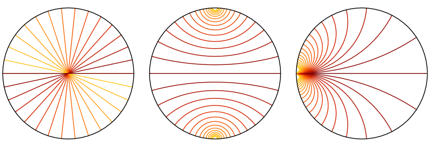
Figure 3: Elements of ${\rm PSL}(2,\mathbb{R})$ can be visualized by their action on geodesics. Some group elements are shown.

The Möbius transformations are conformal mappings, preserving angles. One way to visualize them is through their action on geodesics. Geodesics on the Poincaré disk are circular arcs perpendicular to the boundary. The ${\rm PSL}(2,\mathbb{R})$ symmetry maps geodesics to other geodesics. For example, the $x$-axis diameter is a geodesic. Transformations with $\beta=0$ and $\alpha=e^{i\phi}$ for $\phi\in\mathbb{R}$ are rotations. Transformations with $\beta\neq 0$ move the origin. Some 1-parameter families of transformations are shown in Fig 3. To see the action of these transformations on $a$ and $b$, one can project $a$ and $b$ to the disk, find a geodesic passing through them, transform it, then project back onto the sphere.

We conclude that the BMS equation respects ${\rm PSL}(2,\mathbb{R})$, and so $g_{ab}(L)$ can only depend on the distance between $a$ and $b$ according to the metric on the Poincaré disk. That is, $g_{ab}(L)$ only depends on

$$g_{ab}(L)=g({{\color[rgb]{0.7,0.0,0.0}\langle}{ab}{\color[rgb]{0.7,0.0,0.0}\rangle}},L)=g\left(\frac{(ab)}{2\cos\theta_{i}\cos\theta_{j}},L\right)=g\left(\frac{1-\cos\theta_{ij}}{2\cos\theta_{i}\cos\theta_{j}},L\right)$$ (89)

Because of this property, without loss of generality, we can choose $z_{a}=0$, or $\theta_{a}=0$. That is, we identify $a=\overline{n}$ in the calculation. We therefore only need

$${\color[rgb]{0.7,0.0,0.0}\langle}{\overline{n}j}{\color[rgb]{0.7,0.0,0.0}\rangle}=\frac{1-\cos\theta_{j}}{2\cos\theta_{j}},\qquad{\color[rgb]{0.7,0.0,0.0}\langle}{\overline{n}b}{\color[rgb]{0.7,0.0,0.0}\rangle}=\frac{1-\cos\theta_{b}}{2\cos\theta_{b}}$$ (90)

This greatly simplifies the calculation of the NGLs.

7 Perturbative calculation of NGLs to five loops

While the symmetry of the BMS equation is clearer under stereographic projection, we find it more convenient to perform the integrals over angles. It is convenient to define

$$r_{ij}=\frac{1}{2}\ln\Big{(}1+{\color[rgb]{0.7,0.0,0.0}\langle}{ij}{\color[rgb]{0.7,0.0,0.0}\rangle}\Big{)}=\frac{1}{2}\ln\frac{[ij]}{2\cos\theta_{i}\cos\theta_{j}}$$ (91)

$r_{ij}$ is essentially the 1-loop Sudakov factor, Eq. (71). Then Eq. (73) becomes

$$\partial_{L}g_{\overline{n}b}(L)=\frac{1}{4\pi}\int_{0}^{1}d\cos\theta_{j}\int_{0}^{2\pi}d\phi_{j}\frac{(\overline{n}b)}{(\overline{n}j)(jb)}\left[e^{{L}(r_{\overline{n}b}-r_{\overline{n}j}-r_{jb})}g_{\overline{n}j}(L)g_{jb}(L)-g_{\overline{n}b}(L)\right]$$ (92)

To obtain the $m$-loop NGLs, we expand Eq. (92) recursively. Recalling that $g_{ab}^{(0)}=1$ and $g_{ab}^{(1)}=0$, we get

$$\partial_{L}g^{(2)}_{\overline{n}b}(L)= \frac{1}{4\pi}\int^{1}_{0}d\cos\theta_{j}\int^{2\pi}_{0}d\phi_{j}\frac{(\overline{n}b)}{(\overline{n}j)(jb)}(r_{\overline{n}b}-r_{\overline{n}j}-r_{jb}),$$ (93)

$$\partial_{L}g^{(3)}_{\overline{n}b}(L)= \frac{1}{4\pi}\int^{1}_{0}d\cos\theta_{j}\int^{2\pi}_{0}d\phi_{j}\frac{(\overline{n}b)}{(\overline{n}j)(jb)}\left[\frac{{L}^{2}}{2}(r_{\overline{n}b}-r_{\overline{n}j}-r_{jb})^{2}+g^{(2)}_{\overline{n}j}+g^{(2)}_{jb}-g^{(2)}_{\overline{n}b}\right],$$ (94)

$$\partial_{L}g^{(4)}_{\overline{n}b}(L)= \frac{1}{4\pi}\int^{1}_{0}d\cos\theta_{j}\int^{2\pi}_{0}d\phi_{j}\frac{(\overline{n}b)}{(\overline{n}j)(jb)}$$

$$\times\left[\frac{{L}^{3}}{6}(r_{\overline{n}b}-r_{\overline{n}j}-r_{jb})^{3}+{L}(r_{\overline{n}b}-r_{\overline{n}j}-r_{jb})(g^{(2)}_{\overline{n}j}+g^{(2)}_{jb})+g^{(3)}_{\overline{n}j}+g^{(3)}_{jb}-g^{(3)}_{\overline{n}b}\right]$$ (95)

We note that at each order, there are exactly one azimuthal angle integral and one polar angle integral to be done, once the lower order NGLs are known. Also these integrals are finite, although there are singular denominators at each order.

7.1 Azimuthal integrals

The azimuthal integrals can be performed using contour integration. As a simple yet non-trivial example, consider an azimuthal integral required for the 2-loop NGLs,

$$\Phi_{2}=\int^{2\pi}_{0}\frac{d\phi_{j}}{2\pi}\frac{1}{(jb)}\ln\Big{(}1+{\color[rgb]{0.7,0.0,0.0}\langle}{jb}{\color[rgb]{0.7,0.0,0.0}\rangle}\Big{)}$$ (96)

After the standard change of variables, $t=e^{i\phi_{j}}$, this becomes

$$\Phi_{2}=-\frac{2}{\sin\theta_{j}\sin\theta_{b}}\oint_{C}\frac{dt}{2\pi i}\frac{1}{(t-t_{+})(t-t_{-})}\ln\frac{1+\cos\theta_{j}\cos\theta_{b}-\sin\theta_{j}\sin\theta_{b}\left(\frac{1}{2t}+\frac{t}{2}\right)}{2\cos\theta_{j}\cos\theta_{b}},$$ (97)

where the integral contour is the unit circle, and

$$t_{+}=\frac{1-\cos\theta_{j}\cos\theta_{b}+|\cos\theta_{j}-\cos\theta_{b}|}{\sin\theta_{j}\sin\theta_{b}},\qquad t_{-}=\frac{1-\cos\theta_{j}\cos\theta_{b}-|\cos\theta_{j}-\cos\theta_{b}|}{\sin\theta_{j}\sin\theta_{b}}$$ (98)

The factor $\frac{1}{(t-t_{+})(t-t_{-})}$ contains two single poles, but only the pole at $t_{-}$ is within the unit circle. Furthermore, since $t_{+}$ and $t_{-}$ are the solutions of the equation ${\color[rgb]{0.7,0.0,0.0}\langle}{jb}{\color[rgb]{0.7,0.0,0.0}\rangle}=0$, or more precisely $(jb)=0$, it follows that the logarithmic factor $\ln(1+{\color[rgb]{0.7,0.0,0.0}\langle}{jb}{\color[rgb]{0.7,0.0,0.0}\rangle})$ vanishes at $t_{+}$ and $t_{-}$.

The logarithm function contains a branch cut on the negative real axis. Solving for the inequality ${\color[rgb]{0.7,0.0,0.0}\langle}{jb}{\color[rgb]{0.7,0.0,0.0}\rangle}<-1$, we find that the branch cut in the $t$-complex plane is from $0$ to $t_{c}=\frac{1-\cos\theta_{j}-\cos\theta_{b}+\cos\theta_{j}\cos\theta_{b}}{\sin\theta_{j}\sin\theta_{b}}$. Since the integrand is analytic elsewhere within the unit circle, we can shrink the contour $C$ to $C^{\prime}$ as shown in Fig. 4, without changing the value of the integral. The original azimuthal angle integral is therefore traded for a line integral,

$$\Phi_{2}=\frac{4\pi i}{\sin\theta_{j}\sin\theta_{b}}\int^{t_{c}}_{0}\frac{dt}{2\pi i}\frac{1}{(t-t_{+})(t-t_{-})},$$ (99)

where we have made use of the fact that the discontinuity of log function on the negative real axis is $2\pi i$. This line integral can then be trivially done, giving a simple result

$$\int^{2\pi}_{0}\frac{d\phi_{j}}{2\pi}\frac{1}{(jb)}\ln(1+{\color[rgb]{0.7,0.0,0.0}\langle}{jb}{\color[rgb]{0.7,0.0,0.0}\rangle})=\frac{\Big{(}1+2{\color[rgb]{0.7,0.0,0.0}\langle}{b\overline{n}}{\color[rgb]{0.7,0.0,0.0}\rangle}\Big{)}\Big{(}1+2{\color[rgb]{0.7,0.0,0.0}\langle}{j\overline{n}}{\color[rgb]{0.7,0.0,0.0}\rangle}\Big{)}}{2\Big{(}{\color[rgb]{0.7,0.0,0.0}\langle}{b\overline{n}}{\color[rgb]{0.7,0.0,0.0}\rangle}-{\color[rgb]{0.7,0.0,0.0}\langle}{j\overline{n}}{\color[rgb]{0.7,0.0,0.0}\rangle}\Big{)}}\ln\left(\frac{1+{\color[rgb]{0.7,0.0,0.0}\langle}{b\overline{n}}{\color[rgb]{0.7,0.0,0.0}\rangle}}{1+{\color[rgb]{0.7,0.0,0.0}\langle}{j\overline{n}}{\color[rgb]{0.7,0.0,0.0}\rangle}}\right).$$ (100)

We have introduced $\overline{n}$ into this solution using Eq. (90) to manifest the ${\rm PSL}(2,\mathbb{R})$ invariance.

Figure 4: Integral contour for the $t$ integral

The azimuthal integral required for the 3-loop NGL can be done using the same method. The result is

$$\int^{2\pi}_{0}\frac{d\phi_{j}}{2\pi}\frac{\ln{\color[rgb]{0.7,0.0,0.0}\langle}{jb}{\color[rgb]{0.7,0.0,0.0}\rangle}\ln(1+{\color[rgb]{0.7,0.0,0.0}\langle}{jb}{\color[rgb]{0.7,0.0,0.0}\rangle})+\mathrm{Li}_{2}(-{\color[rgb]{0.7,0.0,0.0}\langle}{jb}{\color[rgb]{0.7,0.0,0.0}\rangle})}{(jb)}=\frac{1}{\cos\theta_{b}-\cos\theta_{j}}\\ \times\left[\ln\frac{1+{\color[rgb]{0.7,0.0,0.0}\langle}{j\overline{n}}{\color[rgb]{0.7,0.0,0.0}\rangle}}{1+{\color[rgb]{0.7,0.0,0.0}\langle}{b\overline{n}}{\color[rgb]{0.7,0.0,0.0}\rangle}}\ln\frac{{\color[rgb]{0.7,0.0,0.0}\langle}{j\overline{n}}{\color[rgb]{0.7,0.0,0.0}\rangle}+{\color[rgb]{0.7,0.0,0.0}\langle}{b\overline{n}}{\color[rgb]{0.7,0.0,0.0}\rangle}+|{\color[rgb]{0.7,0.0,0.0}\langle}{j\overline{n}}{\color[rgb]{0.7,0.0,0.0}\rangle}-{\color[rgb]{0.7,0.0,0.0}\langle}{b\overline{n}}{\color[rgb]{0.7,0.0,0.0}\rangle}|}{2}+\mathrm{Li}_{2}(-{\color[rgb]{0.7,0.0,0.0}\langle}{j\overline{n}}{\color[rgb]{0.7,0.0,0.0}\rangle})-\mathrm{Li}_{2}(-{\color[rgb]{0.7,0.0,0.0}\langle}{b\overline{n}}{\color[rgb]{0.7,0.0,0.0}\rangle})\right].$$ (101)

The 4-loop azimuthal integral is in Appendix A.

For all the azimuthal integrals we consider, the integrand is of uniform transcendentality. The azimuthal integrals are all nonsingular and do not change the transcendentality.

7.2 Polar integrals, GPLs, symbols and coproducts

Once all the azimuthal angle integrals are done, which is straightforward with contour integration, all that remains are the polar angle integrals. It turns out to be useful to make another change of variables using Eq. (90),

$$\int^{1}_{0}d\cos\theta_{j}\frac{(b\overline{n})}{(j\overline{n})}=\int^{\infty}_{0}d{\color[rgb]{0.7,0.0,0.0}\langle}{j\overline{n}}{\color[rgb]{0.7,0.0,0.0}\rangle}\frac{2{\color[rgb]{0.7,0.0,0.0}\langle}{b\overline{n}}{\color[rgb]{0.7,0.0,0.0}\rangle}}{\Big{(}1+2{\color[rgb]{0.7,0.0,0.0}\langle}{b\overline{n}}{\color[rgb]{0.7,0.0,0.0}\rangle}\Big{)}\Big{(}1+2{\color[rgb]{0.7,0.0,0.0}\langle}{j\overline{n}}{\color[rgb]{0.7,0.0,0.0}\rangle}\Big{)}{\color[rgb]{0.7,0.0,0.0}\langle}{j\overline{n}}{\color[rgb]{0.7,0.0,0.0}\rangle}}.$$ (102)

At 2 and 3 loops, the ${\color[rgb]{0.7,0.0,0.0}\langle}{j\overline{n}}{\color[rgb]{0.7,0.0,0.0}\rangle}$ integral can be done straightforwardly using, e.g., Mathematica. To go beyond that, we note that after using partial fractions, the polar integrand has the form of an iterated integral:

$$\int^{1}_{0}d\cos\theta_{j}\frac{(b\overline{n})}{(j\overline{n})}\frac{1}{\cos\theta_{b}-\cos\theta_{j}}=\int^{\infty}_{0}d{\color[rgb]{0.7,0.0,0.0}\langle}{j\overline{n}}{\color[rgb]{0.7,0.0,0.0}\rangle}\left(\frac{1}{{\color[rgb]{0.7,0.0,0.0}\langle}{j\overline{n}}{\color[rgb]{0.7,0.0,0.0}\rangle}}-\frac{1}{{\color[rgb]{0.7,0.0,0.0}\langle}{j\overline{n}}{\color[rgb]{0.7,0.0,0.0}\rangle}-{\color[rgb]{0.7,0.0,0.0}\langle}{b\overline{n}}{\color[rgb]{0.7,0.0,0.0}\rangle}}\right)$$ (103)

This is not surprising, since we are solving the BMS equation by iteration. The iterated form nevertheless suggests that we might be able to exploit recent developments in techniques using coproducts and Goncharov polylogarithms (GPLs) [61, 62] to compute them. We now briefly review some of the relevant mathematics.

Recall that the classical polylogarithms are defined iteratively by

$${\mathrm{Li}}_{k}(x)=\int_{0}^{x}\frac{dt}{t}\,{\mathrm{Li}}_{k-1}(t)$$ (104)

with ${\mathrm{Li}}_{1}(x)=-\ln(1-x)$. The GPLs are defined as a generalization of this

$$G(w_{1},\dots,w_{n};x)=\int^{x}_{0}\frac{dt}{t-w_{1}}G(w_{2},\dots,w_{n};t),$$ (105)

with $G(;x)=1$. The set of $n$ complex numbers $\{w_{1},\dots,w_{n}\}$ is called the index vector of the GPL, where at least one entry is nonzero. In the case that all the entries are zeros, the GPL is defined to be the $n^{\text{th}}$ power of $\ln x$, where $n$ is the length of the index vector, also called the weight of the GPL,

$$G(\underbrace{0,\dots,0}_{n};x)=\frac{1}{n!}\ln^{n}x$$ (106)

Classical polylogarithms consist of a subset of the GPLs,

$$G(\underbrace{a,\cdots,a}_{n};x)=\frac{1}{n!}\ln^{n}\left(1-\frac{x}{a}\right),\qquad G(\underbrace{0,\cdots,0}_{n-1},a;x)=-\mathrm{Li}_{n}\left(\frac{x}{a}\right)$$ (107)

If a given integrand can be written so that the integration variable shows up in the argument of a GPL and not in its index vector, then the result for the integral can simply be read off using Eq. (105). In our case, after the azimuthal integrals are done, the integrands are, in general, complicated combinations of classical polylogarithms. These classical polylogarithms can be converted into GPLs using Eq. (106) and (107). However, the resulting GPLs representation of the integrand will not be in the form of Eq. (105). Instead, the integration variable shows up both in the argument and in the index vector in a complicated manner. It is therefore necessary to use functional identities obeyed by the GPLs to massage the integrand into the canonical form, Eq. (105).

A very useful tool for simplifying the integrand is the technique of symbols [63], first introduced in physics in the simplification of 2-loop 6-particle remainder function in ${\mathcal{N}}=4$ Super Yang-Mills theory [64]. The idea is to map the complicated combination of GPLs to a tensor algebra over the group of rational functions, by computing its symbol. In this way, functional identities obeyed by the GPLs are mapped to simpler algebraic identities. We then simplify the symbol using these algebraic relation and finally reconstruct the original expression in the desired form using its symbol.

The symbol acts naturally on iterated integrals of the form

$$T_{k}=\int_{a}^{b}d\ln R_{1}\circ\cdots\circ d\ln R_{k}$$ (108)

where $R_{i}(t)$ are rational functions. The iteration is defined recursively as

$$\int_{a}^{b}d\ln R_{1}\circ\cdots\circ d\ln R_{k}=\int_{a}^{b}d\ln R_{n}(t)\Big{(}\int_{0}^{t}d\ln R_{1}\circ\cdots\circ d\ln R_{n-1}\Big{)}$$ (109)

Both classical polylogarithms and GPLs, defined by Eqs. (104) and (107), are given by iterated integrals in this category, with $R_{k}(t)=1-t$ and $R_{k}(t)=t-w_{k}$ respectively. The symbol of an iterated integral is denoted as

$${\mathcal{S}}[T_{k}]=R_{1}\otimes\cdots\otimes R_{k}$$ (110)

so that

$${\mathcal{S}}[{\mathrm{Li}}_{k}(x)]=-(1-x)\otimes\underbrace{x\otimes\cdots\otimes x}_{k-1}$$ (111)

and

$$\mathcal{S}\left[G\left(a_{1},\dots,a_{n};x\right)\right]=\left(1-\frac{x}{a_{n}}\right)\otimes\dots\otimes\left(1-\frac{x}{a_{1}}\right)$$ (112)

Another important property of the symbol is that

$$R_{1}\cdots\otimes(R_{a}R_{b})\otimes R_{k}=R_{1}\cdots\otimes R_{a}\otimes\cdots R_{k}+R_{1}\cdots\otimes R_{b}\otimes\cdots R_{k}$$ (113)

and ${\mathcal{S}}[c]=0$ for constants $c$.

As an example, we consider the polar angle integral over the azimuthal-averaged integrand at 3 loops. Specifically, we are interested in the following integral

$$\frac{1}{{L}^{3}}g^{(3)}_{\overline{n}b}(L)=-\frac{1}{24}\int^{\infty}_{0}d{\color[rgb]{0.7,0.0,0.0}\langle}{j\overline{n}}{\color[rgb]{0.7,0.0,0.0}\rangle}\left(\frac{1}{{\color[rgb]{0.7,0.0,0.0}\langle}{j\overline{n}}{\color[rgb]{0.7,0.0,0.0}\rangle}}-\frac{1}{{\color[rgb]{0.7,0.0,0.0}\langle}{j\overline{n}}{\color[rgb]{0.7,0.0,0.0}\rangle}-{\color[rgb]{0.7,0.0,0.0}\langle}{b\overline{n}}{\color[rgb]{0.7,0.0,0.0}\rangle}}\right)\Phi_{3}({\color[rgb]{0.7,0.0,0.0}\langle}{b\overline{n}}{\color[rgb]{0.7,0.0,0.0}\rangle},{\color[rgb]{0.7,0.0,0.0}\langle}{j\overline{n}}{\color[rgb]{0.7,0.0,0.0}\rangle})$$ (114)

$\Phi_{3}({\color[rgb]{0.7,0.0,0.0}\langle}{b\overline{n}}{\color[rgb]{0.7,0.0,0.0}\rangle},{\color[rgb]{0.7,0.0,0.0}\langle}{j\overline{n}}{\color[rgb]{0.7,0.0,0.0}\rangle})$ is a piecewise smooth function of ${\color[rgb]{0.7,0.0,0.0}\langle}{j\overline{n}}{\color[rgb]{0.7,0.0,0.0}\rangle}$ for fixed ${\color[rgb]{0.7,0.0,0.0}\langle}{b\overline{n}}{\color[rgb]{0.7,0.0,0.0}\rangle}$. Let

$$u_{1}={\color[rgb]{0.7,0.0,0.0}\langle}{b\overline{n}}{\color[rgb]{0.7,0.0,0.0}\rangle},\qquad u_{2}={\color[rgb]{0.7,0.0,0.0}\langle}{j\overline{n}}{\color[rgb]{0.7,0.0,0.0}\rangle},$$ (115)

we then have

$$\left.\Phi_{3}(u_{1},u_{2})\right|_{u_{1}>u_{2}}=\ln(1+u_{2})\left(\ln\frac{u_{1}(1+u_{2})}{u_{2}(1+u_{1})}\right),$$ (116)

and

$$\left.\Phi_{3}(u_{1},u_{2})\right|_{u_{1}<u_{2}}=\ln u_{1}\ln(1+u_{1})-2\ln^{2}(1+u_{1})+\ln(1+u_{1})\ln u_{2}+3\ln(1+u_{1})\ln(1+u_{2})\\ -2\ln u_{2}\ln(1+u_{2})-\ln^{2}(1+u_{2})+2\mathrm{Li}_{2}(-u_{1})-2\mathrm{Li}_{2}(-u_{2})$$ (117)

The integral in Eq. (114) is naturally split into two pieces,

$${\mathcal{I}}_{3}=-\frac{1}{24}\int^{u_{1}}_{0}du_{2}\left(\frac{1}{u_{2}}-\frac{1}{u_{2}-u_{1}}\right)\Phi_{3}(u_{1},u_{2})$$ (118)

and

$$\mathcal{J}_{3}=-\frac{1}{24}\int^{\infty}_{u_{1}}du_{2}\left(\frac{1}{u_{2}}-\frac{1}{u_{2}-u_{1}}\right)\Phi_{3}(u_{1},u_{2})$$ (119)

For simplicity, we only show details for the computation of ${\mathcal{I}}_{3}$. $\mathcal{J}_{3}$ can be obtained in almost the same way, after changing variables to move the lower bound of the integration range to $0$.

To proceed, we first compute the symbol of $\left.\Phi_{3}(u_{1},u_{2})\right|_{u_{1}>u_{2}}$,

$${\mathcal{S}}\left[\left.\Phi_{3}(u_{1},u_{2})\right|_{u_{1}>u_{2}}\right]=u_{1}\otimes(1+u_{2})-(1+u_{1})\otimes(1+u_{2})-u_{2}\otimes(1+u_{2})+(1+u_{2})\otimes u_{1}\\ -(1+u_{2})\otimes(1+u_{1})-(1+u_{2})\otimes u_{2}+2\left[(1+u_{2})\otimes(1+u_{2})\right]$$ (120)

It is straightforward to find a set of GPLs with the same symbol. A simple algorithmic approach is given in Ref. [65]. The important observation is that the symbol of a GPL with argument $x$ and an $x$-independent index vector consists of a single term, as in Eq. (112). Note that $x$ shows up in every entry of the symbol in Eq. (112). To match the symbol of Eq. (120), we start from the terms where the next integral variable, $u_{2}$, shows up in every entry of the symbol. For example, the following GPL has exactly the same symbol as the last term in Eq. (120)

$$\mathcal{S}[G(-1,-1;u_{2})]=(1+u_{2})\otimes(1+u_{2})$$ (121)

We then proceed to reconstruct the symbol where at least one entry is independent of $u_{2}$, e.g., $(1+u_{2})\otimes(1+u_{1})$. From Eq. (112) we know that such a symbol cannot correspond to a single GPL where $u_{2}$ only shows up in the argument but not in the index vector. They can, however, arise from the product of two GPLs, $G(-1;u_{2})G(-1;u_{1})$. In fact, the product of GPLs gives not a single term but two terms, which match exactly with part of the symbol in Eq. (120),

$$\mathcal{S}[G(-1;u_{2})G(-1;u_{1})]=(1+u_{2})\otimes(1+u_{1})+(1+u_{1})\otimes(1+u_{2})$$ (122)

Such procedure can be iterated until the entire symbol has been reconstructed. The result is the following ansatz,

$$\Phi^{G}_{3}(u_{1},u_{2})=G(0;u_{1})G(-1;u_{2})-G(-1;u_{1})G(-1;u_{2})\\ -G(-1,0;u_{2})-G(0,-1;u_{2})+2G(-1,-1,u_{2})$$ (123)

However, since the symbol maps all constants to zero, we cannot yet conclude that $\Phi_{3}\left.(u_{1},u_{2})\right|_{u_{1}>u_{2}}=\Phi^{G}_{3}(u_{1},u_{2})$. The two functions have uniform transcendentality, but they may differ by terms of transcendentality $2$, such as $\pi^{2}$, or terms like $i\pi\times\ln$. In our current case, both $\Phi_{3}$ and $\Phi^{G}_{3}$ are real for $u_{1}>u_{2}>0$, so they can not differ by terms like $i\pi\times\ln$. Instead, they could differ by a term proportional to $\pi^{2}$,

$$\left.\Phi_{3}(u_{1},u_{2})\right|_{u_{1}>u_{2}}=\Phi^{G}_{3}(u_{1},u_{2})+c\,\pi^{2}.$$ (124)

The rational number $c$ can be easily fixed by computing the two sides of the above equation numerically for some $u_{1}$ and $u_{2}$. It turns out that $c=0$. We have thus fully reconstructed $\Phi_{3}(u_{1},u_{2})$ for $u_{1}>u_{2}$ into the canonical form, including the constant term.

Now the integral in Eq. (118) can be done almost trivially, using the iterative definition of GPLs, Eq. (105). For example,

$$\int^{u_{1}}_{0}du_{2}\frac{1}{u_{2}-u_{1}}G(-1,0;u_{2})=G(u_{1},-1,0;u_{1})$$ (125)

Here one needs to be careful because the resulting GPL, $G(u_{1},-1,0;u_{1})$, is logarithmically divergent. In general, when the first entry of a GPL coincides with its argument, there is a logarithmic divergence in it, as evident from the iterational definition, Eq. (105). However, since the original integral Eq. (114) is finite, as can be checked numerically, such logarithmic divergences must be spurious and must cancel against similar logarithmic divergences from other terms. A simple method [67] to deal with such spurious logarithmic divergence is to isolate them using shuffle identities of GPLs [68]:

$$G(a_{1},\dots,a_{n_{1}};x)G(a_{n_{1}+1},\dots,a_{n_{1}+n_{2}};x)=\sum_{\sigma\in\Sigma(n_{1},n_{2})}G(a_{\sigma(1)},\dots,\sigma_{n_{1}+n_{2}};x),$$ (126)

where the summation is over all different permutations in which the relative ordering of the sets $\{a_{1},\dots,a_{n_{1}}\}$ and $\{a_{n_{1}+1},\dots,a_{n_{1}+n_{2}}\}$ are preserved. Applying these shuffle identities to $G(u_{2},-1,0;u_{2})$, we obtain

$$G(u_{1},-1,0;u_{1})=G(u_{1};u_{1})G(-1,0;u_{1})-G(-1,u_{1},0;u_{1})-G(-1,0,u_{1};u_{1})$$ (127)

Now the logarithmic divergent term $G(u_{1};u_{1})G(-1,0;u_{1})$ is isolated. The final result for ${\mathcal{I}}_{3}$ is then given by

$${\mathcal{I}}_{3}=\frac{1}{24}G\left(-1;u_{1}\right)G\left(-1,u_{1};u_{1}\right)-\frac{1}{24}G\left(0;u_{1}\right)G\left(-1,u_{1};u_{1}\right)+\frac{1}{24}G\left(-1;u_{1}\right)G\left(0,-1;u_{1}\right)\\ -\frac{1}{24}G\left(0;u_{1}\right)G\left(0,-1;u_{1}\right)-\frac{1}{12}G\left(-1,-1,u_{1};u_{1}\right)+\frac{1}{24}G\left(-1,0,u_{1};u_{1}\right)\\ -\frac{1}{12}G\left(-1,u_{1},-1;u_{1}\right)+\frac{1}{24}G\left(-1,u_{1},0;u_{1}\right)-\frac{1}{12}G\left(0,-1,-1;u_{1}\right)+\frac{1}{24}G\left(0,-1,0;u_{1}\right)\\ +\frac{1}{24}G\left(0,-1,u_{1};u_{1}\right)+\frac{1}{24}G\left(0,0,-1;u_{1}\right)+\frac{1}{24}G\left(0,u_{1},-1;u_{1}\right)$$ (128)

Doing the integral for $\mathcal{J}_{3}$ in the same way, we obtain the final result for Eq. (114),

$$\frac{1}{{L}^{3}}g^{(3)}_{\overline{n}b}(L)=\frac{\pi^{2}}{36}G(-1;u_{1})-\frac{1}{4}G(-1,-1,-1;u_{1})\\ +\frac{1}{4}G(-1,-1,0;u_{1})+\frac{1}{12}G(-1,0,-1;u_{1})-\frac{1}{12}G(-1,0,0;u_{1})$$ (129)

where $u_{1}={\color[rgb]{0.7,0.0,0.0}\langle}{\overline{n}b}{\color[rgb]{0.7,0.0,0.0}\rangle}$. In terms of classical polylogarithms this is

$$g^{(3)}_{\overline{n}b}(L)={L}^{3}\Bigg{[}\frac{\pi^{2}}{72}\ln(1+u_{1})-\frac{1}{24}\ln^{2}u_{1}\ln(1+u_{1})+\frac{1}{12}\ln u_{1}\ln^{2}(1+u_{1})-\frac{1}{36}\ln^{3}(1+u_{1})\\ -\frac{1}{12}\ln u_{1}\mathrm{Li}_{2}(-u_{1})+\frac{1}{12}\ln(1+u_{1})\mathrm{Li}_{2}(-u_{1})+\frac{1}{12}\mathrm{Li}_{3}(-u_{1})-\frac{1}{12}\mathrm{Li}_{3}\left(\frac{1}{1+u_{1}}\right)+\frac{\zeta(3)}{12}\Bigg{]},$$ (130)

This result agrees with what we find by direct integration of the 3-loop integrand using Mathematica.

At 4 loops, the polar integral cannot be done directly, and we find the use of symbols to be necessary. One additional complication beyond 3 loops is that symbols does not fix the functional form of the original function (e.g., there can be terms like $\zeta(2)\log$, which is mapped to zero under the symbol). Fortunately, these terms can be obtained using a generalization of the symbol called the coproduct [63, 69], whose application in the context of scattering amplitudes is nicely demonstrated in Ref. [67]. We provide an example in Appendix C which illustrates the use of the coproduct in our calculation. The result for $g_{ab}^{(4)}(L)$ is given in Appendix B.

7.3 Analytical results for NGLs at fixed order

The formulas for $g_{ab}(L)$ with $a$ and $b$ in the left hemisphere at up to 4 loops are given in Appendix B. When $b$ is in the right hemisphere, aligned with the hemisphere axis $n$, the formulas are simpler. Defining $y={\color[rgb]{0.7,0.0,0.0}\langle}{a\overline{n}}{\color[rgb]{0.7,0.0,0.0}\rangle}=\frac{1-\cos\theta_{a}}{2\cos\theta_{a}}$, we find

$$\frac{1}{{L}^{2}}g^{(2)}_{an}(L)= -\frac{\pi^{2}}{24},$$ (131)

$$\frac{1}{{L}^{3}}g^{(3)}_{an}(L)= \frac{\zeta(3)}{12},$$ (132)

$$\frac{1}{{L}^{4}}g^{(4)}_{an}(L)= \frac{\pi^{4}}{34560}-\frac{\pi^{2}}{576}G(0,-1;y)-\frac{1}{96}G(0,-1,-1,-1;y)+\frac{1}{96}G(0,-1,0,-1;y)$$

$$= \frac{\pi^{4}}{6912}-\frac{1}{576}\ln(-y)\ln^{3}(1+y)+\frac{\pi^{2}}{576}\mathrm{Li}_{2}(-y)+\frac{1}{192}\mathrm{Li}_{2}(-y)^{2}$$

$$-\frac{1}{192}\ln^{2}(1+y)\mathrm{Li}_{2}(1+y)+\frac{1}{96}\ln(1+y)\mathrm{Li}_{3}(1+y)-\frac{1}{96}\mathrm{Li}_{4}(1+y)$$

$$-\frac{1}{48}S_{2,2}(-y),$$ (133)

where the functions $S_{2,2}(-y)$ is the Nielsen polylogarithm.

It is perhaps worth making a few comments about these results and their calculation:

• The perturbative expansion of the NGLs have uniform degree of transcendental weight at each order. At $n$ loops, the transcendentality weight is $n$.

• At 2 and 3 loops, the opposite hemisphere NGLs $g_{an}$ is independent of the dipole directions. There is a low-order accident as there is dependence on ${\color[rgb]{0.7,0.0,0.0}\langle}{an}{\color[rgb]{0.7,0.0,0.0}\rangle}$ at 4 loops and beyond.

• The asymptotic behavior of the NGLs is straightforward to extract. In the limit $x={\color[rgb]{0.7,0.0,0.0}\langle}{ab}{\color[rgb]{0.7,0.0,0.0}\rangle}\to 0$, $a$ and $b$ coincide. In that limit, we find

  $$\lim_{x\to 0}g^{(n)}_{ab}(L)=0+\mathcal{O}(x),\qquad n=2,3,4.$$ (134)

  In the limit of $x\to\infty$, either $a$ or $b$ becomes perpendicular to the hemisphere axis. The asymptotic behavior of the same hemisphere NGLs in that limit is given by

  $$\lim_{x\to\infty}g^{(2)}_{ab}(L)= -\frac{\pi^{2}}{24}{L}^{2}+\mathcal{O}\left(\frac{1}{x}\right),$$ (135)

  $$\lim_{x\to\infty}g^{(3)}_{ab}(L)= \frac{\zeta(3)}{12}{L}^{3}+\mathcal{O}\left(\frac{1}{x}\right),$$ (136)

  $$\lim_{x\to\infty}g^{(4)}_{ab}(L)= \left(-\frac{\pi^{4}}{5760}-\frac{\zeta(3)}{48}\ln x\right){L}^{4}+\mathcal{O}\left(\frac{1}{x}\right),$$ (137)

  For the opposite hemisphere NGLs, the $y\to 0$ limit gives exactly the hemisphere NGLs, because $a$ coincides with $\overline{n}$ in that limit. The $y\to\infty$ limit is given by

  $$\lim_{y\to\infty}g^{(2)}_{an}(L)= -\frac{\pi^{2}}{24}{L}^{2}+\mathcal{O}\left(\frac{1}{y}\right),$$ (138)

  $$\lim_{y\to\infty}g^{(3)}_{an}(L)= \frac{\zeta(3)}{12}{L}^{3}+\mathcal{O}\left(\frac{1}{y}\right),$$ (139)

  $$\lim_{y\to\infty}g^{(4)}_{an}(L)= \left(\frac{\pi^{4}}{5760}-\frac{\zeta(3)}{48}\ln y\right){L}^{4}+\mathcal{O}\left(\frac{1}{y}\right),$$ (140)

  Intriguingly, the opposite hemisphere and same hemisphere NGLs exhibit the same logarithmic divergence for large $x$ or $y$, with the same slope and opposite intercept.

Finally, using the analytic results for the opposite hemisphere and same hemisphere NGLs up to and including 4 loops, we can calculate the hemisphere NGLs through 5 loops. The result is

$$\boxed{g_{n\overline{n}}(L)=1-\frac{\pi^{2}}{24}{L}^{2}+\frac{\zeta(3)}{12}{L}^{3}+\frac{\pi^{4}}{34560}{L}^{4}+\left(-\frac{\pi^{2}\zeta(3)}{360}+\frac{17\zeta(5)}{480}\right){L}^{5}+\dots}$$ (141)

Numerically, it can be written as

$$g_{n\overline{n}}(L)=1-0.411233512{L}^{2}+0.10017141{L}^{3}+0.0028185501{L}^{4}+0.0037694522{L}^{5}+\dots$$ (142)

Note that the 5-loop coefficient is actually larger than the as the 4-loop coefficient. Perhaps this is because the 4-loop coefficient is unusually small. In any case, it suggests that the series may not be convergent beyond ${L}=1$. Plots of the approximations of $g_{n\overline{n}}(L)$ at up to 5 loops and a comparison to the exact (that is, numerically resummed) result are shown in Fig. 5. We discuss the calculation of the resummed result in the next section.

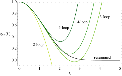
Figure 5: Comparisons of the complete, resummed, leading NGL series for the hemisphere mass distribution, $g_{n\overline{n}}(L)$, to its fixed-order approximation at up to 5 loops. The resummed distribution is computed by numerically solving the BMS equation. The fixed order analytical expansions are given in Eq. (141). On the left, the numerical solution is labelled “resummed”. The right plot shows the fixed order approximations relative to this resummed result in the region $0<{L}<2$.

8 Resummation

An exact solution to the hemisphere BMS equation, Eq. (62), would resum the leading hemisphere NGL. While we cannot solve this equation analytically, finding a numerical solution is straightforward. Before discussing the numerically approach, we explore an iterative approach to the resummed solution, finding an exact solution in the first nontrivial case.

8.1 Two loop resummation

Rather than expanding the BMS equation to fixed order and integrating, we can iterate the equation in an alternative manner. Following [40], we first rewrite Eq. (62) as

$$\partial_{L}g_{ab}(L)=g_{ab}(L)\int_{\text{left}}\frac{d\Omega_{j}}{4\pi}W_{ab}^{j}\left[U_{abj}(L)-1\right]+\int_{\text{left}}\frac{d\Omega_{j}}{4\pi}W_{ab}^{j}U_{abj}(L)\left[g_{aj}(L)g_{jb}(L)-g_{ab}(L)\right]$$ (143)

In this form, the second term on the right-hand side only contributes to the NGLs starting at order $L^{3}$. If we ignore this term, the BMS equation reduces to a linear differential equation which is straightforward to solve. For the opposite-hemisphere case, with $a=n$ and $b=\overline{n}$, we get

$$\partial_{L}g^{(2R)}_{n\overline{n}}(L) =g_{n\overline{n}}^{(2R)}(L)\int_{\text{left}}\frac{d\Omega_{j}}{4\pi}W_{n\overline{n}}^{j}\left[U_{n\overline{n}j}(L)-1\right]$$ (144)

$$=2^{L}\int_{0}^{1}dc\frac{1}{(1-c^{2})}\left[\frac{2^{L}c^{L}}{(1+c)^{L}}-1\right]g_{n\overline{n}}^{(2R)}(L)$$ (145)

$$=-\frac{1}{2}\left(\gamma_{E}+\frac{\Gamma^{\prime}({L})}{\Gamma({L})}+\frac{1}{{L}}\right)g_{n\overline{n}}^{(2R)}(L)$$ (146)

with $\Gamma(L)$ the gamma function. The solution to this differential equation is

$$g^{(2R)}_{n\overline{n}}=\sqrt{\frac{e^{-\gamma_{E}{L}}}{\Gamma(1+{L})}}=1-\frac{\pi^{2}}{24}{L}^{2}+\frac{\zeta(3)}{6}{L}^{3}+\cdots$$ (147)

This partially resummed result is not particularly useful, as it does not dominate the full solution in any particular limit. It nevertheless has some interesting features:

• Unlike the naive exponentiation of the 2-loop results, $g_{ab}=\exp(-\frac{\pi^{2}}{24}{L}^{2})$, the resummed 2-loop result includes odd powers of ${L}$ in its expansion.

• The expansion of this result contains half of the 3-loop leading NGL.

• There is an intriguing formal similarity between this solution and solutions to renormalization group equations for global logarithms (see e.g. [54]). These RGEs are easiest to solve in Laplace space. This suggests there may be a way to solve the BMS equation exactly using some clever integral transform.

A comparison of $g^{(2R)}_{n\overline{n}}$, $g_{ab}=\exp(-\frac{\pi^{2}}{24}{L}^{2})$, the numerically resummed result, and the 5-loop approximation are shown in Fig. 6.

8.2 Numerical resummation

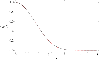
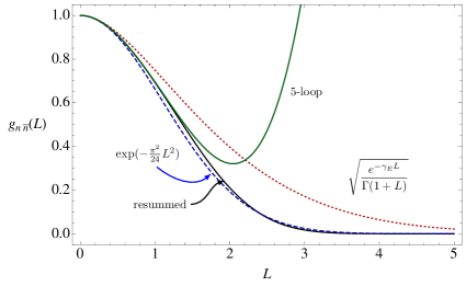
Figure 6: Left shows a comparisons of the resummation of the leading NGL using the Monte Carlo approach of Dasgupta and Salam (dashed, red) to a numerical integration of the BMS equation (black). Right shows a comparison of the numerically integrated result to various approximations.

The BMS equation for the non-global logarithms, in the form of Eqs. (73) and (75) can be solved numerically for $g_{ab}(L)$. Since this equation has only a single derivative, and the boundary condition $g_{ab}(0)=1$ for all $a,b$ is simple, we can solve the equation by simply integrating. As noted in Section 6.2, although $a$ and $b$ are points on the sphere, $g_{ab}$ only depends on the invariant distance ${\color[rgb]{0.7,0.0,0.0}\langle}{ab}{\color[rgb]{0.7,0.0,0.0}\rangle}$ associated with the Poincaré disk after stereographic projection. Rather than exploiting this, we take a more brute-force approach and use only the obvious azimuthal asymmetry: we parameterize $a$ and $b$ by by $\cos\theta_{a}$, $\cos\theta_{b}$ and $\phi_{a}-\phi_{b}$. To solve the BMS equation numerically, we discretize the angles into $n_{\theta}$ and $n_{\phi}$ bins, and solve the equation by summing the integrand with step size $\Delta L={L}/n_{L}$. The computation time using this approach scales like $n_{L}n_{c}^{3}n_{\phi}^{2}$.

The only thing which makes the numerical integration nontrivial is the collinear singularity when $j=a$ of $j=b$. This singularity causes no problem in an analytic integral (it can be integrated over), but must be avoided in a discretized approach. We take the simplest solution and simply omit the $j=a$ and $j=b$ bins. This omission obviously affects the results for finite $n_{c}$, but smoothly disappears as $n_{c}\to\infty$, Rather than trying to take very large $n_{c}$, we simply take values of order $n_{c}=30$ or $n_{c}=40$ and extrapolate to $n_{c}=\infty$ from a fit as a function of $n_{c}$.

Our solution for $g_{n\overline{n}}(L)$ is shown in Fig. 6. On the left side of this figure, it is compared to the numerical calculation of the same quantity by Dasgupta and Salam  [37]. More precisely, we compare to the fit given in their paper, which in our normalization is

$$g_{n\overline{n}}^{\text{(DS)}}(L)=\exp\left[-\frac{\pi^{2}}{24}{L}^{2}\frac{1+0.180625{L}^{2}}{1+0.325472{L}^{1.33}}\right]$$ (148)

In the region $L<1.4$, where the fit in [37] is claimed to be valid, we find less than a $0.1\%$ disparity. This confirms the equivalence of the two approaches. It is notable however that $g_{n\overline{n}}^{\text{(DS)}}(L)$ does not have a series expansion around ${L}=0$. Indeed, at ${L}=0$, the third derivative of this function is zero and the fourth derivative is infinite.

The right side of Fig. 6 compares the resummed distribution to various approximations. It is very interesting that the exponential of the 2-loop leading NGL provides the best approximation. We have no explanation of this fact.

Figure 5 compares the resummed distribution to the $n$-loop approximation, with $n=2,3,4$ and $5$. The series appears not be convergent beyond ${L}\approx 1$.

9 Non-global logarithms at finite $N_{c}$

We have discussed the equivalence of explicit matrix element construction of NGLs and the iterative expansion of BMS equation at large $N_{c}$. We have also discussed the symmetry of the BMS equation. In this section, we briefly discuss the implication of combining these two ingredients at finite $N_{c}$.

An evolution equation describing the evolution of NGLs at finite $N_{c}$ has been conjectured by Weigert [50] and solved numerically by Hatta and Ueda [51]. This conjecture is based on the formal similarity of the BMS equation and BK equation, and that the BK equation has a finite $N_{c}$ generalization, the JIMWLK equation [70, 71, 72]. However, to the best of our knowledge, there is no direct derivation of this evolution equation, nor is there a proof that the equation reproduces all of the leading NGLs at finite $N_{c}$.

It is certainly true that the SEO approximation can be applied at finite $N_{c}$. Instead of dipoles, more involved recursive soft gluon insertion formulas must be used, but one still has physical picture of Wilson lines emitting gluons which then become new Wilson lines. Thus the matrix element construction of the NGL integrand described in Sec. 3 and 4 still applies. A formulation for the recursive picture is discussed in [55, 73] using the recursive soft gluon insertion formula in color space notation [55, 73]. Specifically, the squared amplitudes at finite $N_{c}$ for $m+1$ real soft gluon emissions with SEO from a quark-antiquark dipole $(ab)$ can be obtained from the corresponding amplitudes with the softest gluon removed:

$$\left|M^{1,\dots,m}_{ab}\right|^{2}=-g^{2}\sum_{i,j=a,b,1,\dots,m-1}\int\frac{\omega_{m}d\omega_{m}}{4\pi^{2}}\frac{d\Omega_{m}}{4\pi}\frac{(ij)}{(im)(mj)}\left|M^{(i,j);1,\dots,m-1}_{ab}\right|^{2},$$ (149)

where we have also included the soft phase space factor. The color correlated amplitude $M^{(i,j);1,\dots,m}_{ab}$ is defined as [73]

$$\left|M^{(i,j);1,\dots,m}_{ab}\right|^{2}=\langle M^{1,\dots,m}_{ab}|\boldsymbol{T}_{i}\cdot\boldsymbol{T}_{j}|M^{1,\dots,m}_{ab}\rangle$$ (150)

To make contact with the leading color-squared amplitudes, Eq. (11), we note that the color correlation factorizes into individual color dipoles at large $N_{c}$. In particular, for a color dipole $(ij)$, we have

$$\boldsymbol{T}_{i}+\boldsymbol{T}_{j}\overset{N_{c}\to\infty}{=}0\Rightarrow\boldsymbol{T}_{i}\cdot\boldsymbol{T}_{j}=\left\{\begin{array}[]{l l}-\frac{N_{c}}{2}&\quad i,j=a,b\\ -N_{c}&\quad\text{otherwise}\end{array}\right.$$ (153)

where the factor of $1/2$ in the first case comes from the fact that $C_{F}=\frac{N_{c}}{2}+\mathcal{O}(1/N_{c})$.

Although the color structure is more complicated at finite $N_{c}$, the kinematics of factorization formula in Eq. (149) is not. In particular, the energy integral still trivially factorizes off and the radiator function ${\mathcal{W}}_{ij}^{m}=\frac{(ij)}{(im)(mj)}$ is unchanged. Thus, the real emission integrand still enjoys the full Möbius symmetry, ${\rm PSL}(2,\mathbb{C})$ of the BMS equation. Following the discussion in Sec. 3, it is also easy to see that, since the real-virtual and virtual corrections in the SEO limit are of the same form as the real emission, they also preserve the symmetry. As at finite $N_{c}$, the integration region for the hemisphere NGLs, breaks ${\rm PSL}(2,\mathbb{C})$ down to ${\rm PSL}(2,\mathbb{R})$ symmetry of the Poincaré disk. There is no clear reason why this ${\rm PSL}(2,\mathbb{R})$ symmetry should be further broken. Thus we expect that even at finite $N_{c}$, $g_{ab}(L)$ depends on $a$ and $b$ only though the invariant ${\color[rgb]{0.7,0.0,0.0}\langle}{ab}{\color[rgb]{0.7,0.0,0.0}\rangle}$.

10 Conclusions

In this paper we have explored the structure of the leading non-global logarithmic series for the hemisphere mass distribution in $e^{+}e^{-}$ collisions. The NGLs are represented by functions $g_{ab}(L)$, where $a$ and $b$ are directions of hard colored particles producing the radiation which generates the NGLs. For the $e^{+}e^{-}$ case we take $a$ and $b$ aligned with the hemisphere axis $n$ and $\overline{n}$, and only $g_{n\overline{n}}(L)$ is relevant. In the general case, $a$ and $b$ do not have to be aligned with the hemisphere axis $n$. We consider the more general $g_{ab}(L)$ since it feeds in to $g_{n\overline{n}}$ and since it has interesting symmetry properties.

The leading NGLs can be computed using the strong-energy ordering (SEO) approximation. This approximation simplifies both the real-emission matrix elements as well as contributions to the cross section involving virtual and real-virtual graphs. The SEO has led to the BMS equation [40] which allows for the resummation of the leading NGL. We checked that the real/virtual contributions to the cross section for NGLs agree with the expansion of the BMS equation order-by-order in perturbation theory.

One advantage of using the BMS equation is that it manifests most clearly the ${\rm PSL}(2,\mathbb{C})$ symmetry observed in [59, 60]. We showed that the hemisphere integration region breaks the ${\rm PSL}(2,\mathbb{C})$ symmetry down to ${\rm PSL}(2,\mathbb{R})$ which is the isometry group of the Poincaré disk. Angles on the hemisphere representing ends of a color dipole furnish a representation of ${\rm PSL}(2,\mathbb{R})$ which can be constructed through a stereographic projection onto the equatorial disk. The result is that $g_{ab}(L)$ only depends on a single invariant, the distance ${\color[rgb]{0.7,0.0,0.0}\langle}{ab}{\color[rgb]{0.7,0.0,0.0}\rangle}=\frac{1-\cos\theta_{ab}}{\cos\theta_{a}\cos\theta_{b}}$ between $a$ and $b$, where $\theta_{a}$ and $\theta_{b}$ are the polar angles with respect the hemisphere axis and $\theta_{ab}$ is the angle between them. This invariant greatly simplifies the calculation of the leading NGLs at fixed order.

To compute the fixed-order expansion of the leading hemisphere NGLs, we iterated the BMS equation. At each loop order, only one azimuthal angle and one polar angle integral needs to be done. The azimuthal integrals are straightforward to do by deforming the integration contour. The result at $n$ loops is a set of classical polylogarithms of uniform transcendentality weight $n$. To do the polar angle integrals, we convert these classical polylogarithms into Goncharov polylogarithms in a canonical form using the tensor algebra of the symbol. The symbols gives the complete result up to constants of uniform transcendentality, like $\zeta(n)$ or $\pi^{n}$. At 3 loops, these constants can be guessed, but at 4 loops we require the use of the coproduct to extract them. The result is a formula for $g_{ab}(L)$ at 4 loops. We then use this formula to compute $g_{n\overline{n}}(L)$ at 5 loops. This is our main concrete result, given in Eq. (141).

In addition to computing the leading NGL at 5 loops, we resummed the leading NGL to all orders by solving the BMS equation numerically. We found a result in very good agreement with the fit from a Monte Carlo calculation presented in [37], confirming the equivalence of the BMS equation and the Monte Carlo approach. Interestingly, the resummed distribution seems to agree quite well with the exponentiation of the 2-loop result, despite the apparent importance of the 3-loop NGL coefficient.

The 5-loop leading hemisphere NGL may be of some (limited) phenomenological importance, since it contributes to event shapes like the heavy jet mass [12]. However, more profound consequences of this work probably include the relatively simple structure of the leading NGL series. Working in the strong-energy-ordered approximation apparently produces an extended symmetry which is only partially broken through a finite integration region. That the NGLs are computed with iterated integrals of uniform transcendentality is also somewhat surprising. While such integral series are common in supersymmetric settings, examples in large $N_{c}$ QCD ($\mathcal{N}=0$) are more rare. It may be important to understand the symmetry and the generality of the iterated structure in more depth.

Appendix A Azimuthal integrals

We present some useful formulae for azimuthal integral in this appendix. The 1 and 2-loop results are simple

$$\Phi_{1}=\int^{2\pi}_{0}\frac{d\phi_{j}}{2\pi}\frac{1}{(jb)}=\frac{1}{|\cos\theta_{j}-\cos\theta_{b}|},$$ (154)

$$\Phi_{2}=\int^{2\pi}_{0}\frac{d\phi_{j}}{2\pi}\frac{\ln(1+{\color[rgb]{0.7,0.0,0.0}\langle}{jb}{\color[rgb]{0.7,0.0,0.0}\rangle})}{(jb)}=\frac{1}{\cos\theta_{j}-\cos\theta_{b}}\ln\frac{1+{\color[rgb]{0.7,0.0,0.0}\langle}{b\overline{n}}{\color[rgb]{0.7,0.0,0.0}\rangle}}{1+{\color[rgb]{0.7,0.0,0.0}\langle}{j\overline{n}}{\color[rgb]{0.7,0.0,0.0}\rangle}},$$ (155)

The 3-loop result is more complicated

$$\Phi_{3}=\int^{2\pi}_{0}\frac{d\phi_{j}}{2\pi}\frac{\ln{\color[rgb]{0.7,0.0,0.0}\langle}{jb}{\color[rgb]{0.7,0.0,0.0}\rangle}\ln(1+{\color[rgb]{0.7,0.0,0.0}\langle}{jb}{\color[rgb]{0.7,0.0,0.0}\rangle})+\mathrm{Li}_{2}(-{\color[rgb]{0.7,0.0,0.0}\langle}{jb}{\color[rgb]{0.7,0.0,0.0}\rangle})}{(jb)}=\frac{1}{\cos\theta_{b}-\cos\theta_{j}}\\ \times\left[\ln\frac{1+{\color[rgb]{0.7,0.0,0.0}\langle}{j\overline{n}}{\color[rgb]{0.7,0.0,0.0}\rangle}}{1+{\color[rgb]{0.7,0.0,0.0}\langle}{b\overline{n}}{\color[rgb]{0.7,0.0,0.0}\rangle}}\ln\frac{{\color[rgb]{0.7,0.0,0.0}\langle}{j\overline{n}}{\color[rgb]{0.7,0.0,0.0}\rangle}+{\color[rgb]{0.7,0.0,0.0}\langle}{b\overline{n}}{\color[rgb]{0.7,0.0,0.0}\rangle}+|{\color[rgb]{0.7,0.0,0.0}\langle}{j\overline{n}}{\color[rgb]{0.7,0.0,0.0}\rangle}-{\color[rgb]{0.7,0.0,0.0}\langle}{b\overline{n}}{\color[rgb]{0.7,0.0,0.0}\rangle}|}{2}+\mathrm{Li}_{2}(-{\color[rgb]{0.7,0.0,0.0}\langle}{j\overline{n}}{\color[rgb]{0.7,0.0,0.0}\rangle})-\mathrm{Li}_{2}(-{\color[rgb]{0.7,0.0,0.0}\langle}{b\overline{n}}{\color[rgb]{0.7,0.0,0.0}\rangle})\right].$$ (156)

At 4 loops the result is most usefully expressed in terms of GPLs in canonical form

$$\Phi_{4}= (\cos\theta_{b}-\cos\theta_{j})\int^{2\pi}_{0}\frac{d\phi_{j}}{2\pi(jb)}\left[-\frac{1}{6}r^{3}_{jb}+\frac{1}{L^{3}}g^{(3)}_{jb}(L)-\frac{1}{L^{2}}r_{jb}g^{(2)}_{jb}(L)\right]$$

$$= -\frac{1}{12}G(-1,0,{\color[rgb]{0.7,0.0,0.0}\langle}{b\overline{n}}{\color[rgb]{0.7,0.0,0.0}\rangle};{\color[rgb]{0.7,0.0,0.0}\langle}{j\overline{n}}{\color[rgb]{0.7,0.0,0.0}\rangle})-\frac{1}{12}G(0,-1,{\color[rgb]{0.7,0.0,0.0}\langle}{b\overline{n}}{\color[rgb]{0.7,0.0,0.0}\rangle};{\color[rgb]{0.7,0.0,0.0}\langle}{j\overline{n}}{\color[rgb]{0.7,0.0,0.0}\rangle})+\frac{1}{8}G(-1,0,-1;{\color[rgb]{0.7,0.0,0.0}\langle}{j\overline{n}}{\color[rgb]{0.7,0.0,0.0}\rangle})$$

$$-\frac{1}{24}G(0,-1;{\color[rgb]{0.7,0.0,0.0}\langle}{j\overline{n}}{\color[rgb]{0.7,0.0,0.0}\rangle})G(-1;{\color[rgb]{0.7,0.0,0.0}\langle}{b\overline{n}}{\color[rgb]{0.7,0.0,0.0}\rangle})-\frac{1}{12}G(0,-1;{\color[rgb]{0.7,0.0,0.0}\langle}{j\overline{n}}{\color[rgb]{0.7,0.0,0.0}\rangle})G(0;{\color[rgb]{0.7,0.0,0.0}\langle}{b\overline{n}}{\color[rgb]{0.7,0.0,0.0}\rangle})+\frac{1}{12}G(-1;{\color[rgb]{0.7,0.0,0.0}\langle}{j\overline{n}}{\color[rgb]{0.7,0.0,0.0}\rangle})G(0,0;{\color[rgb]{0.7,0.0,0.0}\langle}{b\overline{n}}{\color[rgb]{0.7,0.0,0.0}\rangle})$$

$$+\frac{1}{24}G(-1;{\color[rgb]{0.7,0.0,0.0}\langle}{j\overline{n}}{\color[rgb]{0.7,0.0,0.0}\rangle})G(0,-1;{\color[rgb]{0.7,0.0,0.0}\langle}{b\overline{n}}{\color[rgb]{0.7,0.0,0.0}\rangle})-\frac{1}{12}G(-1,0,0;{\color[rgb]{0.7,0.0,0.0}\langle}{b\overline{n}}{\color[rgb]{0.7,0.0,0.0}\rangle})-\frac{1}{24}G(-1,0,-1;{\color[rgb]{0.7,0.0,0.0}\langle}{b\overline{n}}{\color[rgb]{0.7,0.0,0.0}\rangle})$$

$$+\frac{\pi^{2}}{36}G(-1;{\color[rgb]{0.7,0.0,0.0}\langle}{b\overline{n}}{\color[rgb]{0.7,0.0,0.0}\rangle})-\frac{\pi^{2}}{36}G(-1;{\color[rgb]{0.7,0.0,0.0}\langle}{j\overline{n}}{\color[rgb]{0.7,0.0,0.0}\rangle}),$$ (157)

which is valid for ${\color[rgb]{0.7,0.0,0.0}\langle}{j\overline{n}}{\color[rgb]{0.7,0.0,0.0}\rangle}>{\color[rgb]{0.7,0.0,0.0}\langle}{b\overline{n}}{\color[rgb]{0.7,0.0,0.0}\rangle}$. This equation is in the canonical GPL form, since the next integration variable ${\color[rgb]{0.7,0.0,0.0}\langle}{j\overline{n}}{\color[rgb]{0.7,0.0,0.0}\rangle}$ shows up only in the argument of GPLs. Some details of how this canonical form is realized are explained in Appendix C.

Appendix B General hemisphere NGL functions to 4 loops

For the same hemisphere NGLs, that is, both $a$ and $b$ are in the left hemisphere, we have obtained the analytical results up to and include four loops. Defining $x={\color[rgb]{0.7,0.0,0.0}\langle}{ab}{\color[rgb]{0.7,0.0,0.0}\rangle}$ we find

$$\frac{1}{{L}^{2}}g^{(2)}_{ab}(L)= -\frac{1}{4}G(-1,-1;x)+\frac{1}{4}G(-1,0;x)$$

$$= \frac{1}{4}\ln x\ln(1+x)-\frac{1}{8}\ln^{2}(1+x)+\mathrm{Li}_{2}(-x),$$ (158)

$$\frac{1}{{L}^{3}}g^{(3)}_{ab}(L)= \frac{\pi^{2}}{36}G(-1;x)-\frac{1}{4}G(-1,-1,-1;x)+\frac{1}{4}G(-1,-1,0;x)+\frac{1}{12}G(-1,0,-1;x)$$

$$-\frac{1}{12}G(-1,0,0;x)$$

$$= \frac{\pi^{2}}{72}\ln(1+x)-\frac{1}{24}\ln^{2}x\ln(1+x)+\frac{1}{12}\ln x\ln^{2}(1+x)-\frac{1}{36}\ln^{3}(1+x)$$

$$-\frac{1}{12}\ln x\mathrm{Li}_{2}(-x)+\frac{1}{12}\ln(1+x)\mathrm{Li}_{2}(-x)+\frac{1}{12}\mathrm{Li}_{3}(-x)-\frac{1}{12}\mathrm{Li}_{3}\left(\frac{1}{1+x}\right)+\frac{\zeta(3)}{12},$$ (159)

$$\frac{1}{{L}^{4}}g^{(4)}_{ab}(L)= \frac{\pi^{2}}{36}G(-1,-1;x)-\frac{\pi^{2}}{144}G(-1,0;x)-\frac{3}{16}G(-1,-1,-1,-1;x)+\frac{3}{16}G(-1,-1,-1,0;x)$$

$$+\frac{1}{12}G(-1,-1,0,-1;x)-\frac{1}{12}G(-1,-1,0,0;x)+\frac{1}{48}G(-1,0,-1,-1;x)$$

$$-\frac{1}{96}G(-1,0,-1,0;x)-\frac{1}{32}G(-1,0,0,-1;x)+\frac{1}{48}G(-1,0,0,0;x)-\frac{\zeta(3)}{16}G(-1;x)$$

$$= -\frac{11\pi^{2}}{576}\ln x\ln(1+x)+\frac{1}{288}\ln^{3}x\ln(1+x)+\frac{\pi^{2}}{72}\ln^{2}(1+x)$$

$$+\frac{1}{24}\ln(-x)\ln(x)\ln^{2}(1+x)-\frac{1}{48}\ln^{2}x\ln^{2}(1+x)+\frac{1}{48}\ln(-x)\ln^{3}(1+x)$$

$$+\frac{1}{32}\ln x\ln^{3}(1+x)-\frac{1}{128}\ln^{4}(1+x)-\frac{\pi^{2}}{144}\mathrm{Li}_{2}(-x)+\frac{1}{96}\ln^{2}x\mathrm{Li}_{2}(-x)$$

$$+\frac{5}{96}\ln^{2}(1+x)\mathrm{Li}_{2}(-x)+\frac{1}{96}\mathrm{Li}_{2}(-x)^{2}+\frac{1}{96}\ln x\ln(1+x)\mathrm{Li}_{2}(1+x)$$

$$+\frac{1}{24}\ln^{2}(1+x)\mathrm{Li}_{2}(1+x)-\frac{1}{48}\ln x\mathrm{Li}_{3}(-x)+\frac{3}{32}\ln(1+x)\mathrm{Li}_{3}(-x)$$

$$+\frac{1}{16}\ln x\mathrm{Li}_{3}(1+x)-\frac{1}{24}\ln(1+x)\mathrm{Li}_{3}(1+x)+\frac{1}{48}\mathrm{Li}_{4}(-x)+\frac{1}{16}S_{2,2}(-x)$$

$$-\frac{\zeta(3)}{16}\ln x-\frac{\zeta(3)}{48}\ln(1+x),$$ (160)

We have given separately the GPL representation and classical polylogarithms representation of the results. The classical polylogarithms representation is obtained using the package HPL [75].

The hemisphere NGL functions $g_{an}(L)$ when one direction is in the right-hemisphere are given in Eq. (131) to (133) .

Appendix C Systematic use of the symbols and coproducts

In this Section we explain how the form of Eq. (157) which is canonical in terms of GPLs is obtained. The azimuthal integral

$$\Phi_{4}=(\cos\theta_{b}-\cos\theta_{j})\int^{2\pi}_{0}\frac{d\phi_{j}}{2\pi(jb)}\left[-\frac{1}{6}r^{3}_{jb}+\frac{1}{L^{3}}g^{(3)}_{jb}(L)-\frac{1}{L^{2}}r_{jb}g^{(2)}_{jb}(L)\right]$$ (161)

can be done using the contour integral method sketched in Section 7 and Mathematica. However, the resulting expression is very complicated and further integrating over ${\color[rgb]{0.7,0.0,0.0}\langle}{j\overline{n}}{\color[rgb]{0.7,0.0,0.0}\rangle}$ is too difficult. However, the symbol of $\Phi_{4}$ is not unmanageable:

$$\mathcal{S}[\Phi_{4}]= \frac{1}{12}{\color[rgb]{0.7,0.0,0.0}\langle}{b\overline{n}}{\color[rgb]{0.7,0.0,0.0}\rangle}\otimes(1+{\color[rgb]{0.7,0.0,0.0}\langle}{b\overline{n}}{\color[rgb]{0.7,0.0,0.0}\rangle})\otimes{\color[rgb]{0.7,0.0,0.0}\langle}{b\overline{n}}{\color[rgb]{0.7,0.0,0.0}\rangle}-\frac{1}{12}{\color[rgb]{0.7,0.0,0.0}\langle}{b\overline{n}}{\color[rgb]{0.7,0.0,0.0}\rangle}\otimes(1+{\color[rgb]{0.7,0.0,0.0}\langle}{b\overline{n}}{\color[rgb]{0.7,0.0,0.0}\rangle})\otimes{\color[rgb]{0.7,0.0,0.0}\langle}{j\overline{n}}{\color[rgb]{0.7,0.0,0.0}\rangle}-\frac{1}{12}{\color[rgb]{0.7,0.0,0.0}\langle}{b\overline{n}}{\color[rgb]{0.7,0.0,0.0}\rangle}\otimes{\color[rgb]{0.7,0.0,0.0}\langle}{j\overline{n}}{\color[rgb]{0.7,0.0,0.0}\rangle}\otimes(1+{\color[rgb]{0.7,0.0,0.0}\langle}{b\overline{n}}{\color[rgb]{0.7,0.0,0.0}\rangle})$$

$$+\frac{1}{12}{\color[rgb]{0.7,0.0,0.0}\langle}{b\overline{n}}{\color[rgb]{0.7,0.0,0.0}\rangle}\otimes{\color[rgb]{0.7,0.0,0.0}\langle}{j\overline{n}}{\color[rgb]{0.7,0.0,0.0}\rangle}\otimes(1+{\color[rgb]{0.7,0.0,0.0}\langle}{j\overline{n}}{\color[rgb]{0.7,0.0,0.0}\rangle})-\frac{1}{24}(1+{\color[rgb]{0.7,0.0,0.0}\langle}{b\overline{n}}{\color[rgb]{0.7,0.0,0.0}\rangle})\otimes{\color[rgb]{0.7,0.0,0.0}\langle}{b\overline{n}}{\color[rgb]{0.7,0.0,0.0}\rangle}\otimes(1+{\color[rgb]{0.7,0.0,0.0}\langle}{b\overline{n}}{\color[rgb]{0.7,0.0,0.0}\rangle})$$

$$+\frac{1}{24}(1+{\color[rgb]{0.7,0.0,0.0}\langle}{b\overline{n}}{\color[rgb]{0.7,0.0,0.0}\rangle})\otimes{\color[rgb]{0.7,0.0,0.0}\langle}{b\overline{n}}{\color[rgb]{0.7,0.0,0.0}\rangle}\otimes(1+{\color[rgb]{0.7,0.0,0.0}\langle}{j\overline{n}}{\color[rgb]{0.7,0.0,0.0}\rangle})+\frac{1}{24}(1+{\color[rgb]{0.7,0.0,0.0}\langle}{b\overline{n}}{\color[rgb]{0.7,0.0,0.0}\rangle})\otimes(1+{\color[rgb]{0.7,0.0,0.0}\langle}{j\overline{n}}{\color[rgb]{0.7,0.0,0.0}\rangle})\otimes{\color[rgb]{0.7,0.0,0.0}\langle}{b\overline{n}}{\color[rgb]{0.7,0.0,0.0}\rangle}$$

$$-\frac{1}{24}(1+{\color[rgb]{0.7,0.0,0.0}\langle}{b\overline{n}}{\color[rgb]{0.7,0.0,0.0}\rangle})\otimes(1+{\color[rgb]{0.7,0.0,0.0}\langle}{j\overline{n}}{\color[rgb]{0.7,0.0,0.0}\rangle})\otimes{\color[rgb]{0.7,0.0,0.0}\langle}{j\overline{n}}{\color[rgb]{0.7,0.0,0.0}\rangle}-\frac{1}{12}({\color[rgb]{0.7,0.0,0.0}\langle}{b\overline{n}}{\color[rgb]{0.7,0.0,0.0}\rangle}-{\color[rgb]{0.7,0.0,0.0}\langle}{j\overline{n}}{\color[rgb]{0.7,0.0,0.0}\rangle})\otimes{\color[rgb]{0.7,0.0,0.0}\langle}{b\overline{n}}{\color[rgb]{0.7,0.0,0.0}\rangle}\otimes(1+{\color[rgb]{0.7,0.0,0.0}\langle}{b\overline{n}}{\color[rgb]{0.7,0.0,0.0}\rangle})$$

$$+\frac{1}{12}({\color[rgb]{0.7,0.0,0.0}\langle}{b\overline{n}}{\color[rgb]{0.7,0.0,0.0}\rangle}-{\color[rgb]{0.7,0.0,0.0}\langle}{j\overline{n}}{\color[rgb]{0.7,0.0,0.0}\rangle})\otimes{\color[rgb]{0.7,0.0,0.0}\langle}{b\overline{n}}{\color[rgb]{0.7,0.0,0.0}\rangle}\otimes(1+{\color[rgb]{0.7,0.0,0.0}\langle}{j\overline{n}}{\color[rgb]{0.7,0.0,0.0}\rangle})-\frac{1}{12}({\color[rgb]{0.7,0.0,0.0}\langle}{b\overline{n}}{\color[rgb]{0.7,0.0,0.0}\rangle}-{\color[rgb]{0.7,0.0,0.0}\langle}{j\overline{n}}{\color[rgb]{0.7,0.0,0.0}\rangle})\otimes(1+{\color[rgb]{0.7,0.0,0.0}\langle}{j\overline{n}}{\color[rgb]{0.7,0.0,0.0}\rangle})\otimes{\color[rgb]{0.7,0.0,0.0}\langle}{b\overline{n}}{\color[rgb]{0.7,0.0,0.0}\rangle}$$

$$+\frac{1}{12}({\color[rgb]{0.7,0.0,0.0}\langle}{b\overline{n}}{\color[rgb]{0.7,0.0,0.0}\rangle}-{\color[rgb]{0.7,0.0,0.0}\langle}{j\overline{n}}{\color[rgb]{0.7,0.0,0.0}\rangle})\otimes(1+{\color[rgb]{0.7,0.0,0.0}\langle}{b\overline{n}}{\color[rgb]{0.7,0.0,0.0}\rangle})\otimes{\color[rgb]{0.7,0.0,0.0}\langle}{j\overline{n}}{\color[rgb]{0.7,0.0,0.0}\rangle}+\frac{1}{12}({\color[rgb]{0.7,0.0,0.0}\langle}{b\overline{n}}{\color[rgb]{0.7,0.0,0.0}\rangle}-{\color[rgb]{0.7,0.0,0.0}\langle}{j\overline{n}}{\color[rgb]{0.7,0.0,0.0}\rangle})\otimes{\color[rgb]{0.7,0.0,0.0}\langle}{j\overline{n}}{\color[rgb]{0.7,0.0,0.0}\rangle}\otimes(1+{\color[rgb]{0.7,0.0,0.0}\langle}{b\overline{n}}{\color[rgb]{0.7,0.0,0.0}\rangle})$$

$$-\frac{1}{12}({\color[rgb]{0.7,0.0,0.0}\langle}{b\overline{n}}{\color[rgb]{0.7,0.0,0.0}\rangle}-{\color[rgb]{0.7,0.0,0.0}\langle}{j\overline{n}}{\color[rgb]{0.7,0.0,0.0}\rangle})\otimes{\color[rgb]{0.7,0.0,0.0}\langle}{j\overline{n}}{\color[rgb]{0.7,0.0,0.0}\rangle}\otimes(1+{\color[rgb]{0.7,0.0,0.0}\langle}{j\overline{n}}{\color[rgb]{0.7,0.0,0.0}\rangle})+\frac{1}{12}({\color[rgb]{0.7,0.0,0.0}\langle}{b\overline{n}}{\color[rgb]{0.7,0.0,0.0}\rangle}-{\color[rgb]{0.7,0.0,0.0}\langle}{j\overline{n}}{\color[rgb]{0.7,0.0,0.0}\rangle})\otimes(1+{\color[rgb]{0.7,0.0,0.0}\langle}{j\overline{n}}{\color[rgb]{0.7,0.0,0.0}\rangle})\otimes{\color[rgb]{0.7,0.0,0.0}\langle}{b\overline{n}}{\color[rgb]{0.7,0.0,0.0}\rangle}$$

$$-\frac{1}{12}({\color[rgb]{0.7,0.0,0.0}\langle}{b\overline{n}}{\color[rgb]{0.7,0.0,0.0}\rangle}-{\color[rgb]{0.7,0.0,0.0}\langle}{j\overline{n}}{\color[rgb]{0.7,0.0,0.0}\rangle})\otimes(1+{\color[rgb]{0.7,0.0,0.0}\langle}{j\overline{n}}{\color[rgb]{0.7,0.0,0.0}\rangle})\otimes{\color[rgb]{0.7,0.0,0.0}\langle}{j\overline{n}}{\color[rgb]{0.7,0.0,0.0}\rangle}-\frac{1}{8}(1+{\color[rgb]{0.7,0.0,0.0}\langle}{j\overline{n}}{\color[rgb]{0.7,0.0,0.0}\rangle})\otimes(1+{\color[rgb]{0.7,0.0,0.0}\langle}{b\overline{n}}{\color[rgb]{0.7,0.0,0.0}\rangle})\otimes{\color[rgb]{0.7,0.0,0.0}\langle}{b\overline{n}}{\color[rgb]{0.7,0.0,0.0}\rangle}$$

$$-\frac{1}{8}(1+{\color[rgb]{0.7,0.0,0.0}\langle}{j\overline{n}}{\color[rgb]{0.7,0.0,0.0}\rangle})\otimes(1+{\color[rgb]{0.7,0.0,0.0}\langle}{b\overline{n}}{\color[rgb]{0.7,0.0,0.0}\rangle})\otimes{\color[rgb]{0.7,0.0,0.0}\langle}{j\overline{n}}{\color[rgb]{0.7,0.0,0.0}\rangle}-\frac{1}{8}(1+{\color[rgb]{0.7,0.0,0.0}\langle}{j\overline{n}}{\color[rgb]{0.7,0.0,0.0}\rangle})\otimes{\color[rgb]{0.7,0.0,0.0}\langle}{j\overline{n}}{\color[rgb]{0.7,0.0,0.0}\rangle}\otimes(1+{\color[rgb]{0.7,0.0,0.0}\langle}{b\overline{n}}{\color[rgb]{0.7,0.0,0.0}\rangle})$$

$$+\frac{1}{8}(1+{\color[rgb]{0.7,0.0,0.0}\langle}{j\overline{n}}{\color[rgb]{0.7,0.0,0.0}\rangle})\otimes{\color[rgb]{0.7,0.0,0.0}\langle}{j\overline{n}}{\color[rgb]{0.7,0.0,0.0}\rangle}\otimes(1+{\color[rgb]{0.7,0.0,0.0}\langle}{j\overline{n}}{\color[rgb]{0.7,0.0,0.0}\rangle}).$$ (162)

From the symbol, we can reconstruct the most complicated part of the original expression, using an algorithm described in Ref. [65]. We start with the terms with the most number of ${\color[rgb]{0.7,0.0,0.0}\langle}{j\overline{n}}{\color[rgb]{0.7,0.0,0.0}\rangle}$ factors. That is, where ${\color[rgb]{0.7,0.0,0.0}\langle}{j\overline{n}}{\color[rgb]{0.7,0.0,0.0}\rangle}$ shows up in all the slots, e.g., $(1+{\color[rgb]{0.7,0.0,0.0}\langle}{j\overline{n}}{\color[rgb]{0.7,0.0,0.0}\rangle})\otimes{\color[rgb]{0.7,0.0,0.0}\langle}{j\overline{n}}{\color[rgb]{0.7,0.0,0.0}\rangle}\otimes(1+{\color[rgb]{0.7,0.0,0.0}\langle}{j\overline{n}}{\color[rgb]{0.7,0.0,0.0}\rangle})$. For each such term, a GPL that has the same symbol can be immediately read off from its entries. For example,

$$\mathcal{S}\Big{[}G(-1,0,-1;{\color[rgb]{0.7,0.0,0.0}\langle}{j\overline{n}}{\color[rgb]{0.7,0.0,0.0}\rangle})\Big{]}=(1+{\color[rgb]{0.7,0.0,0.0}\langle}{j\overline{n}}{\color[rgb]{0.7,0.0,0.0}\rangle})\otimes{\color[rgb]{0.7,0.0,0.0}\langle}{j\overline{n}}{\color[rgb]{0.7,0.0,0.0}\rangle}\otimes(1+{\color[rgb]{0.7,0.0,0.0}\langle}{j\overline{n}}{\color[rgb]{0.7,0.0,0.0}\rangle}).$$ (163)

In this way, we construct an ansatz $\Phi^{G1}_{4}$, consisting of GPLs in the canonical form, whose symbol exactly matches the terms in $\mathcal{S}[\Phi_{4}]$ with the most ${\color[rgb]{0.7,0.0,0.0}\langle}{j\overline{n}}{\color[rgb]{0.7,0.0,0.0}\rangle}$ factors. The symbol of the remainder, $\mathcal{S}(\Phi_{4}-\Phi^{G1}_{4})$ now contains terms where at least one of the slot is free of ${\color[rgb]{0.7,0.0,0.0}\langle}{j\overline{n}}{\color[rgb]{0.7,0.0,0.0}\rangle}$, e.g., $(1+{\color[rgb]{0.7,0.0,0.0}\langle}{j\overline{n}}{\color[rgb]{0.7,0.0,0.0}\rangle})\otimes{\color[rgb]{0.7,0.0,0.0}\langle}{j\overline{n}}{\color[rgb]{0.7,0.0,0.0}\rangle}\otimes(1+{\color[rgb]{0.7,0.0,0.0}\langle}{b\overline{n}}{\color[rgb]{0.7,0.0,0.0}\rangle})$. An ansatz for some terms in of this form might have the symbol

$$\mathcal{S}\Big{[}G(0,-1;{\color[rgb]{0.7,0.0,0.0}\langle}{j\overline{n}}{\color[rgb]{0.7,0.0,0.0}\rangle})G(-1;{\color[rgb]{0.7,0.0,0.0}\langle}{b\overline{n}}{\color[rgb]{0.7,0.0,0.0}\rangle})\Big{]}=(1+{\color[rgb]{0.7,0.0,0.0}\langle}{j\overline{n}}{\color[rgb]{0.7,0.0,0.0}\rangle})\otimes{\color[rgb]{0.7,0.0,0.0}\langle}{j\overline{n}}{\color[rgb]{0.7,0.0,0.0}\rangle}\otimes(1+{\color[rgb]{0.7,0.0,0.0}\langle}{b\overline{n}}{\color[rgb]{0.7,0.0,0.0}\rangle})\\ +(1+{\color[rgb]{0.7,0.0,0.0}\langle}{j\overline{n}}{\color[rgb]{0.7,0.0,0.0}\rangle})\otimes(1+{\color[rgb]{0.7,0.0,0.0}\langle}{b\overline{n}}{\color[rgb]{0.7,0.0,0.0}\rangle})\otimes{\color[rgb]{0.7,0.0,0.0}\langle}{j\overline{n}}{\color[rgb]{0.7,0.0,0.0}\rangle}+(1+{\color[rgb]{0.7,0.0,0.0}\langle}{b\overline{n}}{\color[rgb]{0.7,0.0,0.0}\rangle})\otimes(1+{\color[rgb]{0.7,0.0,0.0}\langle}{j\overline{n}}{\color[rgb]{0.7,0.0,0.0}\rangle})\otimes{\color[rgb]{0.7,0.0,0.0}\langle}{j\overline{n}}{\color[rgb]{0.7,0.0,0.0}\rangle}.$$ (164)

Organizing the matching in this way systematically leads to a guess $\Phi_{4}^{G}$ with GPLs in canonical form with the same symbols as $\Phi_{4}$.

Since $\Phi_{4}$ and $\Phi_{4}^{G}$ have the same symbol, they can only differ by constants of the appropriate transcendentality. For transcendentality-weight $3$ GPLs, the terms missed from the symbol construction can only either be $\zeta(3)$ or could be $\zeta(2)\times\ln[R({\color[rgb]{0.7,0.0,0.0}\langle}{bn}{\color[rgb]{0.7,0.0,0.0}\rangle})]$ for rational functions $R(x)$. The terms proportional to $\zeta(2)$ can be extracted by the coproducts $\Delta_{2,1}$ [67]. Specifically, we have

$$\Delta_{2,1}\Big{[}\Phi_{4}-\Phi^{G}_{4}\Big{]}=\frac{1}{6}\Big{(}\zeta(2)\otimes\ln(1+{\color[rgb]{0.7,0.0,0.0}\langle}{b\overline{n}}{\color[rgb]{0.7,0.0,0.0}\rangle})\Big{)}-\frac{1}{6}\Big{(}\zeta(2)\otimes\ln(1+{\color[rgb]{0.7,0.0,0.0}\langle}{j\overline{n}}{\color[rgb]{0.7,0.0,0.0}\rangle})\Big{)}.$$ (165)

The action of $\Delta_{2,1}$ fixes the terms proportional to $\zeta(2)$. It suggests that we should add

$$\Delta\Phi_{4}^{G}=\frac{\zeta(2)}{6}G(-1;{\color[rgb]{0.7,0.0,0.0}\langle}{b\overline{n}}{\color[rgb]{0.7,0.0,0.0}\rangle})-\frac{\zeta(2)}{6}G(-1;{\color[rgb]{0.7,0.0,0.0}\langle}{j\overline{n}}{\color[rgb]{0.7,0.0,0.0}\rangle}),$$ (166)

to our guess. Finally, one can check at a random phase space point that the difference of $\Phi_{4}$ and $\Phi^{G}_{4}+\Delta\Phi_{4}^{G}$ vanishes, showing that there is no missing $\zeta(3)$ term. The result is Eq. (157).

References

- [1] J. M. Butterworth, A. R. Davison, M. Rubin and G. P. Salam, Phys. Rev. Lett. 100, 242001 (2008) [arXiv:0802.2470 [hep-ph]].
- [2] D. E. Kaplan, K. Rehermann, M. D. Schwartz and B. Tweedie, Phys. Rev. Lett. 101, 142001 (2008) [arXiv:0806.0848 [hep-ph]].
- [3] J. Gallicchio, J. Huth, M. Kagan, M. D. Schwartz, K. Black and B. Tweedie, JHEP 1104, 069 (2011) [arXiv:1010.3698 [hep-ph]].
- [4] J. Thaler and K. Van Tilburg, JHEP 1103, 015 (2011) [arXiv:1011.2268 [hep-ph]].
- [5] Y. Cui, Z. Han and M. D. Schwartz, Phys. Rev. D 83, 074023 (2011) [arXiv:1012.2077 [hep-ph]].
- [6] J. Gallicchio and M. D. Schwartz, Phys. Rev. Lett. 107, 172001 (2011) [arXiv:1106.3076 [hep-ph]].
- [7] S. D. Ellis, A. Hornig, T. S. Roy, D. Krohn and M. D. Schwartz, Phys. Rev. Lett. 108, 182003 (2012) [arXiv:1201.1914 [hep-ph]].
- [8] A. Altheimer, S. Arora, L. Asquith, G. Brooijmans, J. Butterworth, M. Campanelli, B. Chapleau and A. E. Cholakian et al., J. Phys. G 39, 063001 (2012) [arXiv:1201.0008 [hep-ph]].
- [9] S. D. Ellis, A. Hornig, C. Lee, C. K. Vermilion and J. R. Walsh, Phys. Lett. B 689, 82 (2010) [arXiv:0912.0262 [hep-ph]].
- [10] S. D. Ellis, C. K. Vermilion, J. R. Walsh, A. Hornig and C. Lee, JHEP 1011, 101 (2010) [arXiv:1001.0014 [hep-ph]].
- [11] A. Banfi, M. Dasgupta, K. Khelifa-Kerfa and S. Marzani, JHEP 1008, 064 (2010) [arXiv:1004.3483 [hep-ph]].
- [12] Y. -T. Chien and M. D. Schwartz, JHEP 1008, 058 (2010) [arXiv:1005.1644 [hep-ph]].
- [13] R. Kelley, M. D. Schwartz and H. X. Zhu, arXiv:1102.0561 [hep-ph].
- [14] R. Kelley, M. D. Schwartz, R. M. Schabinger and H. X. Zhu, Phys. Rev. D 84, 045022 (2011) [arXiv:1105.3676 [hep-ph]].
- [15] A. Hornig, C. Lee, I. W. Stewart, J. R. Walsh and S. Zuberi, JHEP 1108, 054 (2011) [arXiv:1105.4628 [hep-ph]].
- [16] A. Hornig, C. Lee, J. R. Walsh and S. Zuberi, JHEP 1201, 149 (2012) [arXiv:1110.0004 [hep-ph]].
- [17] K. Khelifa-Kerfa, JHEP 1202, 072 (2012) [arXiv:1111.2016 [hep-ph]].
- [18] R. Kelley, M. D. Schwartz, R. M. Schabinger and H. X. Zhu, Phys. Rev. D 86, 054017 (2012) [arXiv:1112.3343 [hep-ph]].
- [19] A. von Manteuffel, R. M. Schabinger and H. X. Zhu, arXiv:1309.3560 [hep-ph].
- [20] T. Becher and M. D. Schwartz, JHEP 1002, 040 (2010) [arXiv:0911.0681 [hep-ph]].
- [21] R. Kelley and M. D. Schwartz, Phys. Rev. D 83, 033001 (2011) [arXiv:1008.4355 [hep-ph]].
- [22] T. Becher, C. Lorentzen and M. D. Schwartz, Phys. Rev. Lett. 108, 012001 (2012) [arXiv:1106.4310 [hep-ph]].
- [23] H. -n. Li, Z. Li and C. -P. Yuan, Phys. Rev. Lett. 107, 152001 (2011) [arXiv:1107.4535 [hep-ph]].
- [24] I. Feige, M. D. Schwartz, I. W. Stewart and J. Thaler, Phys. Rev. Lett. 109, 092001 (2012) [arXiv:1204.3898 [hep-ph]].
- [25] H. -n. Li, Z. Li and C. -P. Yuan, Phys. Rev. D 87, 074025 (2013) [arXiv:1206.1344 [hep-ph]].
- [26] M. Dasgupta, K. Khelifa-Kerfa, S. Marzani and M. Spannowsky, JHEP 1210, 126 (2012) [arXiv:1207.1640 [hep-ph]].
- [27] T. Becher, C. Lorentzen and M. D. Schwartz, Phys. Rev. D 86, 054026 (2012) [arXiv:1206.6115 [hep-ph]].
- [28] Y. -T. Chien, R. Kelley, M. D. Schwartz and H. X. Zhu, Phys. Rev. D 87, 014010 (2013) [arXiv:1208.0010].
- [29] M. Field, G. Gur-Ari, D. A. Kosower, L. Mannelli and G. Perez, Phys. Rev. D 87, 094013 (2013) [arXiv:1212.2106 [hep-ph]].
- [30] T. T. Jouttenus, I. W. Stewart, F. J. Tackmann and W. J. Waalewijn, Phys. Rev. D 88, 054031 (2013) [arXiv:1302.0846 [hep-ph]].
- [31] H. -M. Chang, M. Procura, J. Thaler and W. J. Waalewijn, Phys. Rev. Lett. 111, 102002 (2013) [arXiv:1303.6637 [hep-ph]].
- [32] A. J. Larkoski, G. P. Salam and J. Thaler, JHEP 1306, 108 (2013) [arXiv:1305.0007 [hep-ph]].
- [33] M. Dasgupta, A. Fregoso, S. Marzani and G. P. Salam, JHEP 1309, 029 (2013) [arXiv:1307.0007 [hep-ph]].
- [34] M. Dasgupta, A. Fregoso, S. Marzani and A. Powling, Eur. Phys. J. C 73, no. 11, 2623 (2013) [arXiv:1307.0013 [hep-ph]].
- [35] A. J. Larkoski, I. Moult and D. Neill, arXiv:1401.4458 [hep-ph].
- [36] A. J. Larkoski, S. Marzani, G. Soyez and J. Thaler, arXiv:1402.2657 [hep-ph].
- [37] M. Dasgupta and G. P. Salam, Phys. Lett. B 512, 323 (2001) [hep-ph/0104277].
- [38] M. Dasgupta and G. P. Salam, JHEP 0203, 017 (2002) [hep-ph/0203009].
- [39] M. Dasgupta and G. P. Salam, JHEP 0208, 032 (2002) [hep-ph/0208073].
- [40] A. Banfi, G. Marchesini and G. Smye, JHEP 0208, 006 (2002) [hep-ph/0206076].
- [41] R. B. Appleby and M. H. Seymour, JHEP 0212, 063 (2002) [hep-ph/0211426].
- [42] G. Marchesini and A. H. Mueller, Phys. Lett. B 575, 37 (2003) [hep-ph/0308284].
- [43] M. Rubin, JHEP 1005, 005 (2010) [arXiv:1002.4557 [hep-ph]].
- [44] A. H. Hoang and S. Kluth, arXiv:0806.3852 [hep-ph].
- [45] C. W. Bauer, S. Fleming, D. Pirjol and I. W. Stewart, Phys. Rev. D 63, 114020 (2001) [hep-ph/0011336].
- [46] C. W. Bauer, D. Pirjol and I. W. Stewart, Phys. Rev. D 65, 054022 (2002) [hep-ph/0109045].
- [47] M. Beneke, A. P. Chapovsky, M. Diehl and T. Feldmann, Nucl. Phys. B 643, 431 (2002) [hep-ph/0206152].
- [48] I. Balitsky, Nucl. Phys. B 463, 99 (1996) [hep-ph/9509348].
- [49] Y. V. Kovchegov, Phys. Rev. D 60, 034008 (1999) [hep-ph/9901281].
- [50] H. Weigert, Nucl. Phys. B 685, 321 (2004) [hep-ph/0312050].
- [51] Y. Hatta and T. Ueda, Nucl. Phys. B 874, 808 (2013) [arXiv:1304.6930 [hep-ph]].
- [52] S. Fleming, A. H. Hoang, S. Mantry and I. W. Stewart, Phys. Rev. D 77, 074010 (2008) [hep-ph/0703207].
- [53] M. D. Schwartz, Phys. Rev. D 77, 014026 (2008) [arXiv:0709.2709 [hep-ph]].
- [54] T. Becher and M. D. Schwartz, JHEP 0807, 034 (2008) [arXiv:0803.0342 [hep-ph]].
- [55] A. Bassetto, M. Ciafaloni and G. Marchesini, Phys. Rept. 100, 201 (1983).
- [56] Y. L. Dokshitzer, V. A. Khoze, A. H. Mueller and S. I. Troian, Gif-sur-Yvette, France: Ed. Frontieres (1991) 274 p. (Basics of)
- [57] A. Bassetto, M. Ciafaloni, G. Marchesini and A. H. Mueller, Nucl. Phys. B 207, 189 (1982).
- [58] K. J. Golec-Biernat and A. M. Stasto, Nucl. Phys. B 668, 345 (2003) [hep-ph/0306279].
- [59] E. Avsar, Y. Hatta and T. Matsuo, JHEP 0906, 011 (2009) [arXiv:0903.4285 [hep-ph]].
- [60] Y. Hatta and T. Ueda, Phys. Rev. D 80, 074018 (2009) [arXiv:0909.0056 [hep-ph]].
- [61] A. B. Goncharov, [arXiv:math/0103059].
- [62] A. B. Goncharov, Math. Res. Lett. 5, 497 (1998) [arXiv:1105.2076 [math.AG]].
- [63] A. B. Goncharov, Duke Math. J. 128, 209 (2005) [arXiv:math/0208144 [math.AG]].
- [64] A. B. Goncharov, M. Spradlin, C. Vergu and A. Volovich, Phys. Rev. Lett. 105, 151605 (2010) [arXiv:1006.5703 [hep-th]].
- [65] C. Anastasiou, C. Duhr, F. Dulat and B. Mistlberger, JHEP 1307, 003 (2013) [arXiv:1302.4379 [hep-ph]].
- [66] C. W. Bauer, A. Frink and R. Kreckel, cs/0004015 [cs-sc].
- [67] C. Duhr, JHEP 1208, 043 (2012) [arXiv:1203.0454 [hep-ph]].
- [68] R. Ree, The Annals of Mathematics (1958) 68, No. 2, pp. 210–220.
- [69] F. Brown, arXiv:1102.1310 [math.NT].
- [70] J. Jalilian-Marian, A. Kovner, L. D. McLerran and H. Weigert, Phys. Rev. D 55, 5414 (1997) [hep-ph/9606337].
- [71] J. Jalilian-Marian, A. Kovner, A. Leonidov and H. Weigert, Phys. Rev. D 59, 014014 (1998) [hep-ph/9706377].
- [72] E. Iancu, A. Leonidov and L. D. McLerran, Phys. Lett. B 510, 133 (2001) [hep-ph/0102009].
- [73] S. Catani and M. Grazzini, Nucl. Phys. B 570, 287 (2000) [hep-ph/9908523].
- [74] V. Del Duca, L. J. Dixon, C. Duhr and J. Pennington, JHEP 1402, 086 (2014) [arXiv:1309.6647 [hep-ph]].
- [75] D. Maître, Comput. Phys. Commun. 174, 222 (2006) [hep-ph/0507152].