Reaction Rate and Composition Dependence of the Stability of Thermonuclear Burning on Accreting Neutron Stars

Abstract

The stability of thermonuclear burning of hydrogen and helium accreted onto neutron stars is strongly dependent on the mass accretion rate. The burning behavior is observed to change from Type I X-ray bursts to stable burning, with oscillatory burning occurring at the transition. Simulations predict the transition at a ten times higher mass accretion rate than observed. Using numerical models we investigate how the transition depends on the hydrogen, helium, and CNO mass fractions of the accreted material, as well as on the nuclear reaction rates of $3\alpha$ and the hot-CNO breakout reactions ${}^{15}\mathrm{O}\left(\alpha,\gamma\right)\mathrm{{}^{19}Ne}$ and ${}^{18}\mathrm{Ne}\left(\alpha,p\right)\mathrm{{}^{21}Na}$. For a lower hydrogen content the transition is at higher accretion rates. Furthermore, most experimentally allowed reaction rate variations change the transition accretion rate by at most $10\,\%$. A factor ten decrease of the ${}^{15}\mathrm{O}\left(\alpha,\gamma\right)\mathrm{{}^{19}Ne}$ rate, however, produces an increase of the transition accretion rate of $35\,\%$. None of our models reproduce the transition at the observed rate, and depending on the true ${}^{15}\mathrm{O}\left(\alpha,\gamma\right)\mathrm{{}^{19}Ne}$ reaction rate, the actual discrepancy may be substantially larger. We find that the width of the interval of accretion rates with marginally stable burning depends strongly on both composition and reaction rates. Furthermore, close to the stability transition, our models predict that X-ray bursts have extended tails where freshly accreted fuel prolongs nuclear burning.

1. Introduction

The thin envelope of neutron stars in low-mass X-ray binaries (LMXBs) is continuously replenished by Roche-lobe overflow of the companion star. The hydrogen- and helium-rich material is quickly compressed, and after mere hours the density and temperature required for thermonuclear burning can be reached (Woosley & Taam, 1976; Maraschi & Cavaliere, 1977; Joss, 1977; Lamb & Lamb, 1978). If a thermonuclear runaway ensues, the unstable burning engulfs the entire atmosphere, consuming most hydrogen and helium within seconds. This powers the frequently observed Type I X-ray bursts (Grindlay et al. 1976; Belian et al. 1976; see also Cornelisse et al. 2003; Galloway et al. 2008; for reviews see Lewin et al. 1993; Strohmayer & Bildsten 2006).

For LMXBs accretion rates, $\dot{M}$, are inferred of up to the Eddington limit of approximately $\dot{M}_{\mathrm{Edd}}\sim 10^{-8}\,M_{\odot}\mathrm{year^{-1}}$ (see Section 2). At high rates close to this limit, the high heating rate from compression and nuclear burning as well as the fast inflow of new fuel allow for steady-state burning of hydrogen and helium (e.g., Fujimoto et al. 1981; Bildsten 1998). A lower burst rate and ultimately an absence of bursts is observed at increasingly large $\dot{M}$, roughly between $0.1\dot{M}_{\mathrm{Edd}}$ and $0.3\dot{M}_{\mathrm{Edd}}$ (Van Paradijs et al., 1988; Cornelisse et al., 2003). When the burst rate is reduced, the presence of steady-state burning becomes evident from an increase of the $\alpha$ parameter, i.e., the ratio of the persistent X-ray fluence between subsequent bursts and the burst fluence: there is an increase in the fraction of fuel that burns in a stable manner (Van Paradijs et al., 1988). Understanding the burning regimes at different $\dot{M}$ allows us to accurately predict the composition of the burning ashes that form the neutron star crust, which has observable consequences for, e.g., the cooling of X-ray transients (e.g., Schatz et al., 2014).

Whereas observations place the transition of stability around $0.1\dot{M}_{\mathrm{Edd}}$ to $0.3\dot{M}_{\mathrm{Edd}}$ , models predict it to occur at a mass accretion rate, $\dot{M}_{\mathrm{st}}$, close to $\dot{M}_{\mathrm{Edd}}$ (Fujimoto et al., 1981). The observed $\dot{M}$ is determined from the persistent X-ray flux. As material from the companion star falls to the neutron star, most of the rotational and gravitational energy is dissipated at the inner region of the accretion disk and at a boundary layer close to the neutron star surface. This causes these regions to thermally emit soft X-rays, and Compton scattering in a corona is thought to produce X-rays in the classical band (e.g., Done et al., 2007). The broad-band X-ray flux is, therefore, used to infer $\dot{M}$. There is some uncertainty in the efficiency of converting the liberated gravitational potential energy to X-rays, as well as obscuration of the X-ray emitting regions by the disk. These uncertainties, however, are generally believed to be at most several tens of percents, whereas the discrepancy is close to an order of magnitude (see also the discussion in Keek et al., 2006). This discrepancy is one of the main challenges for neutron star envelope models.

At the transition, nuclear burning is marginally stable and produces oscillations in the light curve (Heger et al., 2007b). This has been identified with mHz quasi-periodic oscillations (mHz QPOs) observed from hydrogen-accreting neutron stars, which typically occur at accretion rates close to $0.1\,\dot{M}_{\mathrm{Edd}}$ (Revnivtsev et al., 2001; Altamirano et al., 2008; Linares et al., 2012).

In the neutron star envelope hydrogen burns through the hot-CNO cycle (e.g., Wallace & Woosley, 1981), and helium burns through the $3\alpha$ process. At temperatures above $T\gtrsim 5\times 10^{8}\,\mathrm{K}$, breakout from the CNO cycle occurs through the ${}^{15}\mathrm{O}\left(\alpha,\gamma\right)\mathrm{{}^{19}Ne}$ reaction, and for $T\gtrsim 6\times 10^{8}\,\mathrm{K}$ through ${}^{18}\mathrm{Ne}\left(\alpha,p\right)\mathrm{{}^{21}Na}$. This is followed by long chains of $(\alpha,p)$ and $(p,\gamma)$ reactions (the $\alpha$p-process; Van Wormer et al. 1994) as well as $(p,\gamma)$ reactions and $\beta$-decays (the rp-process). Isotopes are produced with mass numbers as high as $108$ (Schatz et al. 2001; for further discussion about the end point see Koike et al. 2004; Elomaa et al. 2009). Detailed numerical studies implement these processes in large nuclear networks (e.g., Woosley et al., 2004; Fisker et al., 2008; José et al., 2010). The importance of key nuclear reactions, such as ${}^{15}\mathrm{O}\left(\alpha,\gamma\right)\mathrm{{}^{19}Ne}$, has been demonstrated for the stability of nuclear burning (Fisker et al., 2006; Cooper & Narayan, 2006b; Fisker et al., 2007; Parikh et al., 2008; Davids et al., 2011; Keek et al., 2012). Especially for the two breakout reactions the rates are poorly constrained by nuclear experiment (Davids et al., 2011; Mohr & Matic, 2013), and experimental work to improve this is ongoing (e.g., Tan et al., 2007, 2009; Salter et al., 2012; He et al., 2013).

In this paper we investigate the dependence of $\dot{M}_{\mathrm{st}}$ on the reaction rates of the $3\alpha$-process and the CNO-cycle breakout reactions ${}^{15}\mathrm{O}\left(\alpha,\gamma\right)\mathrm{{}^{19}Ne}$ and ${}^{18}\mathrm{Ne}\left(\alpha,p\right)\mathrm{{}^{21}Na}$, as well as on the composition of the accreted material.

2. Numerical Methods

The multi-zone simulations of the neutron star envelope presented in this paper are created with the one-dimensional implicit hydrodynamic code KEPLER (Weaver et al., 1978). Nuclear burning is implemented using a large adaptive network (Rauscher et al., 2003). Two sets of simulations are made with different versions of KEPLER, both of which have been used in previous similar studies (Woosley et al., 2004; Heger et al., 2007b, a; Keek et al., 2012). Here we describe the main features of these simulations, and we refer to previous publications for a complete description of the code.

We model the envelope on top of a neutron star with a $1.4\,M_{\odot}$ gravitational mass and a radius of $10\,\mathrm{km}$. No general relativistic corrections are applied, but the Newtonian gravity in our model is the same as the general relativistic gravitational acceleration in the rest frame of the surface of a star of equal gravitational mass with a radius of $11.2\,\mathrm{km}$. The corresponding gravitational redshift of $1+z\simeq 1.26$ is not applied to the presented results and light curves (see also Keek & Heger, 2011). This allows for easier translation to other choices of neutron star properties with the same local gravity. Note, however, that the corrected $\dot{M}$ for an observer at infinity differs from our model value by less than a percent (Keek & Heger, 2011).

The inner part of our model consists of a $2\times 10^{25}\,\mathrm{g}$ ⁵⁶Fe substrate, which acts as an inert thermal buffer. At the bottom boundary of that layer we set a constant luminosity into the envelope originating from heating by electron capture and pycnonuclear reactions in the crust (Haensel & Zdunik, 1990, 2003; Gupta et al., 2007). For each set of simulations we assume a fixed amount of heat per accreted nucleon, $Q_{\mathrm{b}}$, enters the envelope. As such the luminosity at the inner boundary is proportional to the mass accretion rate: $L_{\mathrm{crust}}=Q_{\mathrm{b}}\dot{M}$.

On top of the substrate, we accrete hydrogen- and helium-rich material. We express $\dot{M}$ as a fraction of the Eddington limited mass accretion rate for material of solar composition, $\dot{M}_{\mathrm{Edd}}\equiv 1.75\times 10^{-8}\,M_{\odot}\mathrm{yr^{-1}}$. For easier comparison of values between different models, we use this rate even when the composition deviates from solar.

2.1. Models with nuclear reaction rate variation

To study the effect of key nuclear reaction rates on $\dot{M}_{\mathrm{st}}$, we create models where individual rates are varied within the experimental uncertainties. We use the thermonuclear reaction rate compilation REACLIB $2.0$ (Cyburt et al., 2010). In particular, ${}^{15}\mathrm{O}\left(\alpha,\gamma\right)\mathrm{{}^{19}Ne}$ is taken from Davids et al. (2011; DC11), ${}^{18}\mathrm{Ne}\left(\alpha,p\right)\mathrm{{}^{21}Na}$ from Matic et al. (2009; MV09), and $3\alpha$ from Caughlan & Fowler (1988; CF88). Note that revised formulations of the $3\alpha$ rate exist, but within the temperature range relevant for our simulations the rate is dominated by resonant capture, and the difference is at most $4\%$ (e.g., Fynbo et al., 2005).

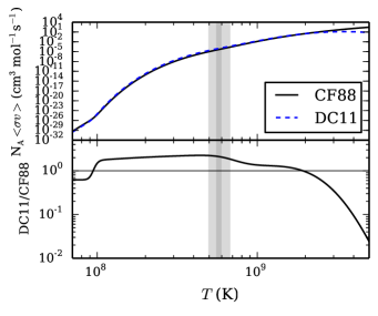
Figure 1.— The temperature dependent part of the ${}^{15}\mathrm{O}\left(\alpha,\gamma\right)\mathrm{{}^{19}Ne}$ reaction rate, $N_{\mathrm{A}}\left\langle\sigma v\right\rangle$, as a function of temperature, $T$, (top), and the ratio of two rates (bottom) from Caughlan & Fowler (1988; CF88) and Davids et al. (2011; DC11). The gray bands indicate the temperature ranges from two models of marginally stable burning (Figure 7), and the horizontal line helps guide the eye for a ratio of $1$.

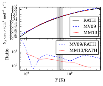
Figure 2.— Same as Figure 1 for the ${}^{18}\mathrm{Ne}\left(\alpha,p\right)\mathrm{{}^{21}Na}$ reaction rate from Rauscher & Thielemann (2000; RATH), Matic et al. (2009; MV09), and Mohr & Matic (2013; MM13).

Figure 3.— Light curves for models closest to the transition to stability, with standard reaction rates and indicated mass accretion rates. The simulation in the lower panel initially exhibits bursts, but quickly transitions to stable burning. The bursts exhibit extended tails.

Figures 1 and 2 illustrate the ${}^{15}\mathrm{O}\left(\alpha,\gamma\right)\mathrm{{}^{19}Ne}$ and ${}^{18}\mathrm{Ne}\left(\alpha,p\right)\mathrm{{}^{21}Na}$ rates, and compare them to the rates used in our second set of models (Section 2.2), as well as to the recent study by Mohr & Matic (2013) for the latter rate. We both increase and decrease the rates of the two CNO breakout reactions by a factor $10$ (e.g., Davids et al., 2011; Mohr & Matic, 2013), and the $3\alpha$ rate by $20\,\%$ (e.g., Austin, 2005), which we regard as the respective ranges of values allowed by nuclear experiment.

The outer zone of the models has a mass of $10^{16}\,\mathrm{g}$, and we use $Q_{\mathrm{b}}=0.1\,\mathrm{MeV\,nucleon^{-1}}$. Accretion is simulated by increasing the mass and updating the composition of the zones that form the outer $2\times 10^{20}\,\mathrm{g}$ of the model, and compressional heating is taken into account (Keek & Heger, 2011). These zones are close to the surface, well above the depth where hydrogen and helium burning takes place. The accreted material is of solar composition with mass fractions of $X=0.71$ (¹H), $Y=0.27$ (⁴He), and $Z=0.02$ (¹⁴N). The latter is quickly converted by the hot-CNO cycle into mostly ¹⁴O and ¹⁵O. Using ¹⁴N as a proxy for all accreted CNO has numerical advantages. Moreover, all the CNO has to be assumed to have been processed to ¹⁴N in the donor star prior to accretion in the case of enhanced $Y$ (e.g., Section 2.2) or if the accretion layer originates deep inside the donor. Keeping the same metal composition for all models allows for easier comparison. For simplicity we do not include other metals in the accretion composition.

2.2. Models with composition variation

To study the effect of the accretion composition on $\dot{M}_{\mathrm{st}}$, we employ a set of simulations that was created with an earlier version of KEPLER. Some of the simulations were presented in previous studies (Woosley et al., 2004; Heger et al., 2007b, a). The basic setup of the models is the same as for the previously discussed set (Section 2.1), with the exception of the following.

Thermonuclear rates are used from a compilation by Rauscher et al. (2003). In particular, ${}^{15}\mathrm{O}\left(\alpha,\gamma\right)\mathrm{{}^{19}Ne}$ and $3\alpha$ are taken from CF88, and ${}^{18}\mathrm{Ne}\left(\alpha,p\right)\mathrm{{}^{21}Na}$ from Rauscher & Thielemann (2000, RATH; Figures 1 and 2).

For these models the outer zone has a mass of $2\times 10^{19}\,\mathrm{g}$, which is well above the depth where H/He burning takes place, and $Q_{\mathrm{b}}=0.15\,\mathrm{MeV\,nucleon^{-1}}$. Accretion is simulated by increasing the pressure at the outer boundary each time step by the weight of the newly accreted material until enough mass for a new zone has accumulated. Then an extra zone is added at the outside of the grid. The addition of a zone induces a brief dip in the light curve as the zone is added with the same temperature as the previous outermost zone and the temperature structure of the model has to adjust. We carefully check that these dips do not influence our results.

We create models for several values of the metallicity of the accreted material, $Z$ (¹⁴N), to represent the initial stellar abundances of donor stars of different metallicity. We determine the ⁴He mass fraction from the crude scaling relation $Y=0.24+1.76Z$, such that for $Z=0$ the Big Bang Nucleosynthesis value is obtained, and for $Z=0.02$ the solar value is reproduced (Section 2.1; see, e.g., West & Heger 2013 and references therein for more advanced composition scaling relations). The remainder of the composition is ¹H: $X=1-Y-Z$. One may rewrite these equations to obtain a relation between $X$ and $Z$:

$$Z=0.362\left(0.76-X\right).$$ (1)

Our metallicity range extends up to $10$ times solar, which may be applicable to some extreme cases towards the Galactic Bulge, or cases of binary mass transfer from the evolved primary star (now the neutron star) to the companion (now the donor). In Section 4.2 we compare the results of the two sets of models and confirm their consistency.

3. Results

3.1. Nuclear reaction rate dependence

We perform $243$ simulations to study the dependence of $\dot{M}_{\mathrm{st}}$ on three key reaction rates. We take steps in $\dot{M}$ to locate the transition between stable and unstable burning. The smallest steps are $0.01\,\dot{M}_{\mathrm{Edd}}$. Figure 3 shows for the standard reaction rates two light curves of models around the stability transition that differ in $\dot{M}$ by the smallest step: $\dot{M}=1.07\,\dot{M}_{\mathrm{Edd}}$ (top panel) and $\dot{M}=1.08\,\dot{M}_{\mathrm{Edd}}$ (bottom panel). The light curves include the start of the simulations, when the nuclear burning has not settled in its final behavior. The first burst is more energetic, as the subsequent bursts ignite in an environment rich in burst ashes (compositional inertia, Taam, 1980). The bursts appear to have an extended tail, as some of the freshly accreted fuel prolongs the burning: approximately $75\%$ of the fluence is emitted in the long tail, where we define the start of the tail where the flux drops below $25\%$ of the value at the burst peak. For the model with $\dot{M}=1.07\,\dot{M}_{\mathrm{Edd}}$, the $\alpha$-parameter measures on average $\alpha=96$.

3.1.1 Convergence of burning behavior

The transition takes place in a small interval of $\dot{M}$. Because we initialize the models without nuclear burning, the first simulated bursts heat up the model slightly, which changes the burning burning behavior somewhat. When we are close to the transition, this initial heating changes the behavior to stable burning. For $\dot{M}=1.09\,\dot{M}_{\mathrm{Edd}}$ $2$ bursts appear before burning becomes stable, whereas for $\dot{M}=1.08\,\dot{M}_{\mathrm{Edd}}$ this number increases to $6$. We continue the simulation with $\dot{M}=1.07\,\dot{M}_{\mathrm{Edd}}$ until $40$ flashes are produced. There is variation in the recurrence time of subsequent bursts: the fractional burst-to-burst variation drops below $5\,\%$ after $5$ bursts, and afterwards the mean variation is $1.4\,\%$. In principle the burning might still turn stable after a larger number of bursts. The steepness of the increase with $\dot{M}$ of the number of bursts before stable burning, however, and the drop in recurrence time variations after $5$ bursts, give us confidence that we are close to the true transition when we choose to create at least $12$ flashes per simulation. Simulations with stable burning are continued for a similar physical time as simulations with bursts.

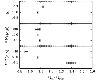
Figure 4.— For different reaction rate variations, the mass accretion rates where models transition from bursts to stable burning, $\dot{M}_{\mathrm{st}}$. Left side of each range is the last bursting model, and the right side is the first stable model. Tick marks in between indicate models with marginally stable burning.

3.1.2 Variations with reaction rates

The change in $\dot{M}_{\mathrm{st}}$ is at most $10\%$, with the exception of the simulations where the ${}^{15}\mathrm{O}\left(\alpha,\gamma\right)\mathrm{{}^{19}Ne}$ rate is scaled by $0.1$: $\dot{M}_{\mathrm{st}}$ is increased by $35\,\%$ (Figure 4). The interval $\Delta\dot{M}_{\mathrm{st}}$ where burning is marginally stable increases for both variations of the ${}^{15}\mathrm{O}\left(\alpha,\gamma\right)\mathrm{{}^{19}Ne}$ rate and for the increased ${}^{18}\mathrm{Ne}\left(\alpha,p\right)\mathrm{{}^{21}Na}$ rate. In the other series of simulations $\Delta\dot{M}_{\mathrm{st}}$ is smaller than our minimum step size. The ${}^{15}\mathrm{O}\left(\alpha,\gamma\right)\mathrm{{}^{19}Ne}$ downward variation yields the largest $\Delta\dot{M}_{\mathrm{st}}$, which allows us to study in detail the changes in the burning behavior and the corresponding light curves (Figure 5). Similar to Figure 3 the burning behavior changes from bursts with extended tails to stable burning. In between, at the boundary of stability, marginally stable burning produces oscillations in the light curve. In this regime the onset of runaway burning is repeatedly quenched when the cooling rate catches up with the burning rate. At higher $\dot{M}$ the oscillations have a smaller amplitude and are more symmetric.

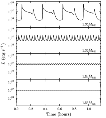
Figure 5.— Light curves for models close to and at the stability transition, with the decreased ${}^{15}\mathrm{O}\left(\alpha,\gamma\right)\mathrm{{}^{19}Ne}$ rate and mass accretion rates indicated as a multiple of $\dot{M}_{\mathrm{Edd}}$. The full simulations last $6.9$ hours each.

We quantify the properties of the oscillations in the light curves of all simulations with marginally stable burning by determining the period, $P$, the relative amplitude, $A$, and the ratio of the duration of the tail and the rise (Figure 6). $A$ is defined as half the luminosity difference between the maxima and minima, normalized by their mean ($A=1$ when the oscillations account for $100\,\%$ of the luminosity). The duration of the rise is the time from a luminosity minimum to the next maximum; the tail duration is analogously defined. At higher $\dot{M}$ both $P$ and $A$ are lower, and the oscillations become more symmetric. The trends are similar for all three series of simulations where we find marginally stable burning.

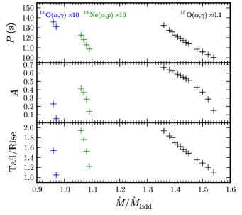
Figure 6.— For the three series of models that exhibit oscillations (Figure 4) the period $P$, relative amplitude $A$, and the ratio of the tail and rise times as a function of mass accretion rate $\dot{M}$. Crosses only indicate the location of data points; no uncertainty is implied.

3.1.3 Nuclear burning at the stability transition

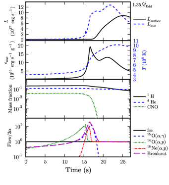
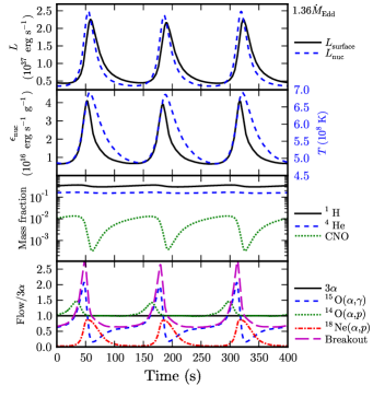
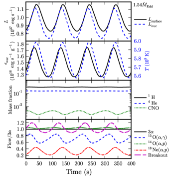
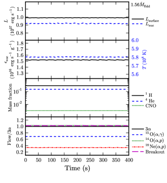
Figure 7.— From the series of simulations with the decreased ${}^{15}\mathrm{O}\left(\alpha,\gamma\right)\mathrm{{}^{19}Ne}$ rate we show details for all models in Figure 5, with $\dot{M}$ indicated in the top right of each panel. For each model, from top to bottom, we give the surface luminosity $L$ and total nuclear energy generation rate $L_{\mathrm{nuc}}$, as well as at the depth where the time-averaged specific nuclear energy generation rate $\epsilon_{\mathrm{nuc}}$ is maximal, $\epsilon_{\mathrm{nuc}}$, temperature $T$ (dashed line), hydrogen, helium, and CNO mass fractions, and several important nuclear flows relative to the $3\alpha$ flow, where ‘breakout’ is the sum of ${}^{15}\mathrm{O}\left(\alpha,\gamma\right)\mathrm{{}^{19}Ne}$ and ${}^{18}\mathrm{Ne}\left(\alpha,p\right)\mathrm{{}^{21}Na}$.

We study in detail four models from the series with the reduced ${}^{15}\mathrm{O}\left(\alpha,\gamma\right)\mathrm{{}^{19}Ne}$ rate around the stability transition (Figures 5 and 7). The highest accretion rate at which we find bursts is $\dot{M}=1.35\,\dot{M}_{\mathrm{Edd}}$, and $\dot{M}=1.56\,\dot{M}_{\mathrm{Edd}}$ is the lowest rate with stable burning. Burning is marginally stable between $\dot{M}=1.36\,\dot{M}_{\mathrm{Edd}}$ and $\dot{M}=1.54\,\dot{M}_{\mathrm{Edd}}$ (Figure 4). Apart from the surface luminosity, $L$, and the total nuclear energy generation rate (neutrino losses subtracted), $L_{\mathrm{nuc}}$, we study several quantities at a fixed column depth where the time-averaged $\epsilon_{\mathrm{nuc}}$ (the specific nuclear energy generation rate; neutrino losses subtracted) is maximal, which is close to the bottom of the hydrogen layer. For the different models this location is between column depths $y=6.2\times 10^{7}\,\mathrm{g\,cm^{-2}}$ and $y=1.1\times 10^{8}\,\mathrm{g\,cm^{-2}}$.

The four simulations have several features in common: there is a delay of several seconds between $L_{\mathrm{nuc}}$ and $L$, because the surface responds on a thermal timescale to changes in the nuclear burning at the bottom of the fuel layer. $L_{\mathrm{nuc}}$ is typically lower than $L$ by $\sim 7\,\%$. The extra emitted energy comes from compressional heating and crustal heating. These contributions are substantial because of the high mass accretion rates. There is also a short delay between $\epsilon_{\mathrm{nuc}}$ and $L_{\mathrm{nuc}}$ because the latter includes nuclear energy generation in neighboring zones to which the burning spreads. Burning in neighboring zones also causes $T$ to remain high for several seconds when $\epsilon_{\mathrm{nuc}}$ starts to decline.

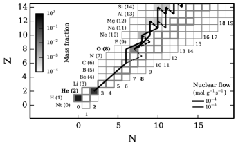
Figure 8.— Net nuclear reaction flow for part of our network during marginally stable burning (at $t=177\,\mathrm{s}$ for $\dot{M}=1.36\,\dot{M}_{\mathrm{Edd}}$ in Figure 7 at the depth where the time-averaged specific nuclear energy generation is maximal). Each square is an isotope with neutron number $N$ and charge number $Z$, with a color indicative of its mass fraction; stable isotopes have thick borders. Lines indicate the flow by nuclear reactions: solid lines flow to higher $Z$ and dashed lines to lower $Z$. A continuous logarithmic distribution of line widths represents the strength of the flows down to $1\%$ of the maximum; the legend shows two line widths as example.

Next we discuss the burning behavior and reaction flows of each simulation. Figure 8 shows the nuclear flow from the model with $\dot{M}=1.36\,\dot{M}_{\mathrm{Edd}}$, but the path of the flow is instructive for understanding all four models. The diagram shows ${}^{4}\mathrm{He}$ burning to ${}^{12}\mathrm{C}$ through the $3\alpha$ process; ${}^{1}\mathrm{H}$ burns via the hot CNO cycle, which is extended with the bicycle through ${}^{14}\mathrm{O}\left(\alpha,p\right)^{17}\mathrm{F}$; breakout from this cycle occurs via ${}^{15}\mathrm{O}\left(\alpha,\gamma\right)\mathrm{{}^{19}Ne}$ and ${}^{18}\mathrm{Ne}\left(\alpha,p\right)\mathrm{{}^{21}Na}$. From ${}^{21}\mathrm{Na}$ there is no net flow back to the CNO cycle, and the nuclear reactions continue towards heavier isotopes through the rp-process (proton captures and $\beta^{+}$-decays). The nuclear flow of Type I bursts has been studied in great detail before (e.g., Woosley et al., 2004; Fisker et al., 2008; José et al., 2010). Here we investigate the part that is responsible for the stability of the burning processes.

For $\dot{M}=1.35\,\dot{M}_{\mathrm{Edd}}$ burning is unstable. Here we only study the burst onset when the thermonuclear runaway and the breakout from the CNO cycle ensues (see Woosley et al. 2004 for a comprehensive study of X-ray burst models with the KEPLER code). The burst starts with thermonuclear runaway burning of helium in the $3\alpha$-process, raising the temperature such that an increasing part of the nuclear flow proceeds through ${}^{14}\mathrm{O}\left(\alpha,p\right)^{17}\mathrm{F}$. Note that we show the flows relative to the $3\alpha$ flow (Figure 7). When $T>4.5\times 10^{8}\,\mathrm{K}$, the breakout flow from the hot CNO cycle via ${}^{15}\mathrm{O}\left(\alpha,\gamma\right)\mathrm{{}^{19}Ne}$ exceeds the $3\alpha$ flow: CNO is destroyed faster than it is created, and its mass fraction starts to decline. The temperature continues to increase, and when $T\simeq 6.2\times 10^{8}\,\mathrm{K}$ the breakout flow through ${}^{18}\mathrm{Ne}\left(\alpha,p\right)\mathrm{{}^{21}Na}$ equals that of ${}^{15}\mathrm{O}\left(\alpha,\gamma\right)\mathrm{{}^{19}Ne}$. Within seconds CNO is depleted. Nuclear burning continues with the $\alpha$p- and rp-processes. The rp-process waiting point at ³⁰S produces a dip in $\epsilon_{\mathrm{nuc}}$, which is visible as a ‘shoulder’ in $L$ (see also Woosley et al., 2004).

For stable burning at $\dot{M}=1.56\,\dot{M}_{\mathrm{Edd}}$ the temperature in the burning layer is $T=5.8\times 10^{8}\,\mathrm{K}$. At this temperature both ${}^{15}\mathrm{O}\left(\alpha,\gamma\right)\mathrm{{}^{19}Ne}$ and ${}^{18}\mathrm{Ne}\left(\alpha,p\right)\mathrm{{}^{21}Na}$ contribute substantially to the CNO breakout, with the former being the largest. The breakout flow equals the $3\alpha$ flow: CNO is destroyed as quickly as it is produced. In the models of marginally stable burning ($\dot{M}=1.36\,\dot{M}_{\mathrm{Edd}}$ and $\dot{M}=1.54\,\dot{M}_{\mathrm{Edd}}$) the various quantities oscillate around the corresponding values in the stable burning model.

For $\dot{M}=1.36\,\dot{M}_{\mathrm{Edd}}$ the oscillations in the $3\alpha$ nuclear flow follow the changes in $T$. In the minima the ${}^{14}\mathrm{O}\left(\alpha,p\right)^{17}\mathrm{F}$ flow follows $3\alpha$ closely. The $3\alpha$ reactions enlarge the CNO mass fraction, which increases the ${}^{14}\mathrm{O}\left(\alpha,p\right)^{17}\mathrm{F}$ flow. This means hydrogen is burned at an increasing rate in the hot CNO cycle as long as the flow through the breakout reactions is relatively small. Once $T$ increases, the ${}^{15}\mathrm{O}\left(\alpha,\gamma\right)\mathrm{{}^{19}Ne}$ and ${}^{18}\mathrm{Ne}\left(\alpha,p\right)\mathrm{{}^{21}Na}$ flows increase: the former becomes larger than $3\alpha$ and the CNO mass fraction declines. This strongly reduces the ${}^{15}\mathrm{O}\left(\alpha,\gamma\right)\mathrm{{}^{19}Ne}$ flow and returns ${}^{14}\mathrm{O}\left(\alpha,p\right)^{17}\mathrm{F}$ to trace $3\alpha$. When the ${}^{18}\mathrm{Ne}\left(\alpha,p\right)\mathrm{{}^{21}Na}$ flow exceeds the ${}^{15}\mathrm{O}\left(\alpha,\gamma\right)\mathrm{{}^{19}Ne}$ flow, $\epsilon_{\mathrm{nuc}}$ peaks and starts to decrease. This is because the chain ${}^{18}\mathrm{Ne}(\beta^{+})^{18}\mathrm{F}(p,\alpha)^{15}\mathrm{O}(\alpha,\gamma)^{19}\mathrm{Ne}(p,\gamma)^{20}\mathrm{Na}(p,\gamma)^{21}\mathrm{Mg}(\beta^{+})^{21}\mathrm{Na}$ releases $20.6\,\mathrm{MeV}$, whereas the direct reaction ${}^{18}\mathrm{Ne}\left(\alpha,p\right)\mathrm{{}^{21}Na}$ generates a mere $2.6\,\mathrm{MeV}$. The difference is that the former effectively converts protons into a ⁴He nucleus and releases the mass difference between the protons and ⁴He, although some energy is carried away by neutrinos and the two $\beta^{+}$-decays. These decays also limit the speed at which the process can operate, such that at higher $T$ it can no longer compete with the direct reaction. Even though $T$ still increases for a brief time, $\epsilon_{\mathrm{nuc}}$ decreases. Once the combined flow through the breakout reactions is reduced below $3\alpha$, the CNO mass fraction increases again. During the oscillations the ${}^{1}\mathrm{H}$ fraction changes locally by $26\,\%$ and the ${}^{4}\mathrm{He}$ fraction by $11\,\%$.

For $\dot{M}=1.54\,\dot{M}_{\mathrm{Edd}}$, during the oscillations the ${}^{1}\mathrm{H}$ fraction changes locally by $3\,\%$ and the ${}^{4}\mathrm{He}$ fraction by $2\,\%$. Similar to the model with $\dot{M}=1.36\,\dot{M}_{\mathrm{Edd}}$, the CNO mass fraction grows or shrinks depending on whether the $3\alpha$ or the breakout flow is larger. Unlike that model, $T$ remains high enough all the time such that ${}^{18}\mathrm{Ne}\left(\alpha,p\right)\mathrm{{}^{21}Na}$ is never switched off. The ${}^{18}\mathrm{Ne}\left(\alpha,p\right)\mathrm{{}^{21}Na}$ flow never exceeds ${}^{15}\mathrm{O}\left(\alpha,\gamma\right)\mathrm{{}^{19}Ne}$, although the relative contribution of the two reactions to the total breakout does change periodically. The result is oscillations in the light curve that have a smaller amplitude and are more symmetric than for $\dot{M}=1.36\,\dot{M}_{\mathrm{Edd}}$, which produces less symmetric oscillations, because of the faster destruction of CNO by the breakout reactions.

3.1.4 Energy generation rate and composition

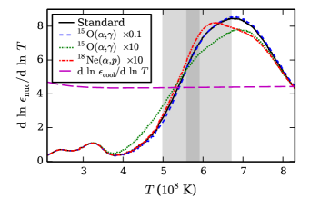
Figure 9.— Temperature dependence of the specific nuclear energy generation rate $\epsilon_{\mathrm{nuc}}$ for different sets of reaction rates. The gray bands indicate the temperature ranges from two models with marginally stable burning (Figure 7).

Stability of thermonuclear burning is often determined by comparing the temperature dependence of the specific nuclear energy generation rate, $\mathrm{d}\ln\epsilon_{\mathrm{nuc}}/\mathrm{d}\ln T$, to that of the specific cooling rate, $\mathrm{d}\ln\epsilon_{\mathrm{cool}}/\mathrm{d}\ln T$ (e.g., Bildsten 1998). From the simulations with the standard rate set we select the stable burning model with the lowest $\dot{M}$ (Figure 3). In the zone of maximal specific energy generation, we calculate $\mathrm{d}\ln\epsilon_{\mathrm{nuc}}/\mathrm{d}\ln T$ for each set of reaction rates, such that in each calculation we use the same composition and we only probe the changes because of the reaction rates (Figure 9). For the rate set with the largest change in $\dot{M}_{\mathrm{st}}$, ${}^{15}\mathrm{O}\left(\alpha,\gamma\right)\mathrm{{}^{19}Ne}$ scaled by $0.1$, $\mathrm{d}\ln\epsilon_{\mathrm{nuc}}/\mathrm{d}\ln T$ is very close to the result for the standard rates, whereas larger deviations are found for rate sets that have smaller changes in $\dot{M}_{\mathrm{st}}$. We also calculate $\mathrm{d}\ln\epsilon_{\mathrm{cool}}/\mathrm{d}\ln T$, which is close to $4.4$ in the temperature range of interest, slightly higher than the value of $4.0$ expected from simple radiative cooling with $\epsilon_{\mathrm{cool}}\propto T^{4}$ (e.g., Bildsten, 1998).

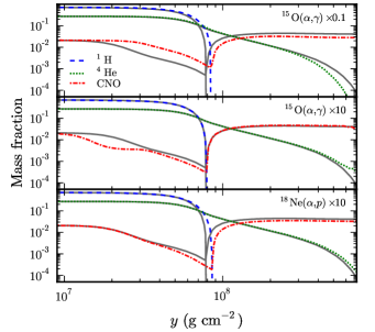
Figure 10.— Mass fractions of ¹H, ⁴He, and CNO as a function of column depth, $y$, for stable burning models with different sets of reaction rates. Solid lines indicate the composition for the standard set of reaction rates.

When reaction rates are changed, this has consequences for the composition as a function of depth during stable burning. Figure 10 shows the differences in the composition profiles for the first models with stable burning (Figure 4) for the reaction rate variations that yield the largest differences in burning behavior from our standard set of rates.

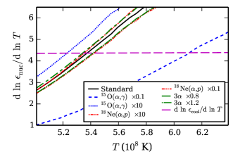
Figure 11.— Temperature dependence of the specific nuclear energy generation rate $\epsilon_{\mathrm{nuc}}$ for different sets of reaction rates zoomed-in on the stability transition. For each rate variation we show the first model with stable burning (Figure 4), which means each curve is for a different equilibrium composition (Figure 10).

For these and similar models for all other rate variations, we calculate the temperature dependence of $\epsilon_{\mathrm{nuc}}$ (Figure 11). The cooling rate’s temperature sensitivity, $\mathrm{d}\ln\epsilon_{\mathrm{cool}}/\mathrm{d}\ln T$, is the same for all models within the temperature range of interest. The range of values of $T$ where $\mathrm{d}\ln\epsilon_{\mathrm{nuc}}/\mathrm{d}\ln T=\mathrm{d}\ln\epsilon_{\mathrm{cool}}/\mathrm{d}\ln T$ is wider than when we calculated $\mathrm{d}\ln\epsilon_{\mathrm{nuc}}/\mathrm{d}\ln T$ with the same composition (Figure 9). Different reaction rates lead, therefore, to changes in the equilibrium composition for stable burning, and the composition has a large influence on the stability of nuclear burning. Note that we found for the reduced ${}^{15}\mathrm{O}\left(\alpha,\gamma\right)\mathrm{{}^{19}Ne}$ rate that the model with stable burning (Figure 7, $\dot{M}=1.56\,\dot{M}_{\mathrm{Edd}}$) has a temperature of $T=5.8\times 10^{8}\,\mathrm{K}$ in the zone of maximal specific energy generation, whereas $\mathrm{d}\ln\epsilon_{\mathrm{nuc}}/\mathrm{d}\ln T=\mathrm{d}\ln\epsilon_{\mathrm{cool}}/\mathrm{d}\ln T$ at $T=6.1\times 10^{8}\,\mathrm{K}$. This exemplifies the limitations of using a one-zone criterion for determining the stability of thermonuclear burning in a multi-zone model.

3.2. Compositional dependence

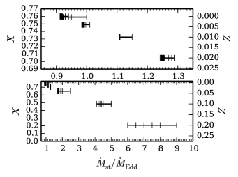
Figure 12.— Similar to Figure 4 for different compositions indicated by $X$ and $Z$. The top panel is a zoom-in of the bottom panel. In highly sampled regions the tick marks are indistinguishable from each other.

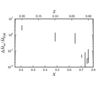
Figure 13.— For different compositions indicated by $X$ and $Z$, the width of the mass accretion region where models transition from bursts to stable burning, $\Delta\dot{M}_{\mathrm{st}}$. The error bar reflects the maximum step size of the simulation grid (see also Figure 12).

The effect of varying the accretion composition is investigated using a large set of $472$ simulations. The multi-zone simulations presented by Heger et al. (2007b) are included in this set ($X=0.759$, $Z=0.001$). For combinations of decreasing $X$ and increasing $Z$ the transition moves to higher values of $\dot{M}_{\mathrm{st}}$ (Figure 12), and the width of the transition, $\Delta\dot{M}_{\mathrm{st}}$, increases (Figure 13). The trend in $\Delta\dot{M}_{\mathrm{st}}$ as a function of composition appears bimodal, as $\Delta\dot{M}_{\mathrm{st}}$ changes by an order of magnitude around $X\simeq 0.65$.

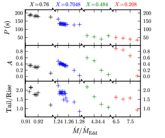
Figure 14.— Same as Figure 6 for four series of models with different accretion compositions as indicated with the hydrogen mass fraction $X$. Note the breaks in the horizontal axis.

For four series of simulations (four accretion compositions) we study the properties of the oscillations in the luminosity (Figure 14). These simulations suffer from small dips in the light curve, which prevents us from determining the properties with the same precision as for the simulations in Section 3.1. This produces a small amount of noise in Figure 14. Nevertheless, the trends in the properties are clearly similar to those in the previous series of models (Figure 6): for larger $\dot{M}$, $P$ and $A$ are smaller, and the oscillations are more symmetric. Values of $P$ range from $34\,\mathrm{s}$ to $189\,\mathrm{s}$, and oscillations with vanishingly small amplitudes are completely symmetric with respect to the rise and the tail. Furthermore, models with a lower hydrogen mass-fraction produce oscillations with on average a shorter period.

3.3. Matching the observed transition

None of the presented models reproduce the transition at the observed $\dot{M}_{\mathrm{st}}$. We investigate whether extrapolation of the trends implied by our models suggests that a certain reaction rate or accretion composition does find $\dot{M}_{\mathrm{st}}=0.1\dot{M}_{\mathrm{Edd}}$.

We have performed simulations for three rate variations of each reaction (Section 3.1). Even though this is a limited number, we use the implied trends to find how large a change in the different rates is required to match observations. One needs to either reduce the $3\alpha$ rate or increase the ${}^{18}\mathrm{Ne}\left(\alpha,p\right)\mathrm{{}^{21}Na}$ or ${}^{15}\mathrm{O}\left(\alpha,\gamma\right)\mathrm{{}^{19}Ne}$ rate by over $4$ orders of magnitude (Figure 4). This is far outside the values allowed by nuclear experiment.

A naive linear extrapolation of the models with different accretion composition finds $\dot{M}_{\mathrm{st}}=0.1\dot{M}_{\mathrm{Edd}}$ is reproduced for $X\simeq 0.9$. In our prescription for the composition this implies a negative metallicity and, therefore, these solutions are unphysical.

In conclusion, although the extrapolations from the results of our simulations are crude, they suggest that no allowed change in accretion composition or reaction rate results in a stability transition at the observed $\dot{M}_{\mathrm{st}}$.

4. Discussion

One of the largest challenges for the theory of thermonuclear burning in the neutron star envelope is to resolve the discrepancy between models/theory and observations on the mass accretion rate where stable burning sets in, $\dot{M}_{\mathrm{st}}$. Using large sets of one-dimensional multi-zone simulations we investigate the dependence of $\dot{M}_{\mathrm{st}}$ on the reaction rates of the $3\alpha$- and CNO breakout processes, as well as on the accretion composition. Although we find that the dependence can be strong, the simulations are unable to reproduce the observed value of $\dot{M}_{\mathrm{st}}$.

4.1. Reaction rates

Hydrogen burns faster in the rp-process than in the $\beta$-limited CNO cycle. A higher $3\alpha$ rate increases the ¹²C mass fraction and boosts CNO cycle burning, reducing the fraction of ¹H that burns in the faster rp-process. Higher breakout rates, on the other hand, reduce the CNO mass fraction, causing the opposite effect. This results in an increased $\dot{M}_{\mathrm{st}}$ for a larger $3\alpha$ rate, whereas the trend is reversed for the two breakout reactions (Figure 4).

The only reaction rate variation that changes $\dot{M}_{\mathrm{st}}$ by more than $10\,\%$ is ${}^{15}\mathrm{O}\left(\alpha,\gamma\right)\mathrm{{}^{19}Ne}$ scaled by $0.1$, with $\dot{M}_{\mathrm{st}}=1.455\,\dot{M}_{\mathrm{Edd}}$. This leads us further from the observed $\dot{M}_{\mathrm{st}}\simeq 0.1\,\dot{M}_{\mathrm{Edd}}$. The discrepancy with observations is, therefore, not resolved by the uncertainty in the considered reaction rates, and it may be substantially larger depending on the actual ${}^{15}\mathrm{O}\left(\alpha,\gamma\right)\mathrm{{}^{19}Ne}$ rate.

The important role of ${}^{15}\mathrm{O}\left(\alpha,\gamma\right)\mathrm{{}^{19}Ne}$ in the stability of thermonuclear burning has been highlighted in several previous studies. Cooper & Narayan (2006b) found from a stability analysis that a reduced rate lowers $\dot{M}_{\mathrm{st}}$ substantially (see also Cooper & Narayan, 2006a). This was, however, in the context of so-called delayed-detonation bursts (Narayan & Heyl, 2003), which are not reproduced by multi-zone simulations (such as the ones in this paper).

In multi-zone models where the ${}^{15}\mathrm{O}\left(\alpha,\gamma\right)\mathrm{{}^{19}Ne}$ rate is orders of magnitude lower than what we considered (effectively switching off CNO breakout), Fisker et al. (2006) identified a stable burning regime over a wide range of $\dot{M}$ (see also Fisker et al., 2007). This precludes X-ray bursts from occurring at any $\dot{M}$. In an attempt to reproduce this, Davids et al. (2011) performed a relatively short multi-zone simulation with a reduced ${}^{15}\mathrm{O}\left(\alpha,\gamma\right)\mathrm{{}^{19}Ne}$ rate (using a different implementation than Fisker et al., 2006), and found flashes instead of the stable burning. This regime is not constrained by our models, because we focus on larger $\dot{M}$, and we do not consider ${}^{15}\mathrm{O}\left(\alpha,\gamma\right)\mathrm{{}^{19}Ne}$ rates as low is in these studies.

Compared to Fisker et al. (2007), we substantially improve on resolving $\dot{M}_{\mathrm{st}}$ for three variations of the ${}^{15}\mathrm{O}\left(\alpha,\gamma\right)\mathrm{{}^{19}Ne}$ rate.

4.2. Accretion Composition

Although the specific energy generation rate for hot CNO burning depends solely on $Z$, the total nuclear energy generation rate increases monotonically with $X$ for a given $\dot{M}$. Models with a lower $X$ (larger $Y,\,Z$), therefore, need to make up for the lower CNO-cycle heating rate with a larger $\dot{M}_{\mathrm{st}}$ (Figure 12). Extrapolation of the $\dot{M}_{\mathrm{st}}(X)$ trend suggests that the observed value is reached for a metal-poor composition with $X\simeq 0.9$. Hydrogen mass fractions higher than the primordial value of $0.76$, however, are not likely to occur in nature except if there is significant spallation during the accretion process (Bildsten et al., 1992). Furthermore, compositional inertia may preclude such a solution from working in practice, as a burst ignites in the presence of the CNO-rich ashes produced in the previous flash (Taam, 1980; Woosley et al., 2004).

Heger et al. (2007b) employ one-zone calculations to study the effect of both $X$ and the gravitational acceleration, $g$, on stability. They argue that $Z$ has a weak effect on the transition accretion rate, and, therefore, keep it at the solar value when varying $X$. For two presented models with the same Newtonian gravitational acceleration as our models ($g_{14}=1.9$), $\dot{M}_{\mathrm{st}}$ increases by approximately a factor $1.8$ when changing from $X=0.7$ to $X=0.5$, whereas a similar change in $X$ for our models increases the transitional rate by a factor $3.6$ (Figure 12). The one-zone model with reduced $X$ has more helium than our corresponding multi-zone model, so with respect to the energy that can be liberated by nuclear burning of the accreted material, the difference between the models with $X=0.7$ and $X=0.5$ is smaller for the one-zone than for our multi-zone models. This may explain why the difference in transitional mass accretion rate is also smaller for the one-zone models.

To check the self-consistency of the set of models with composition variation and the set with reaction rate variation, consider the models from the former with $X=0.7048$ and $Z=0.02$, which is close to the composition used in the latter set. The two sets used different prescriptions for the CNO breakout reaction rates (Figures 1, 2). Using simple interpolation of the $\dot{M}_{\mathrm{st}}$ values in Figure 4 to derive a scaling for $\dot{M}_{\mathrm{st}}$ of the composition variation set yields $\dot{M}_{\mathrm{st}}=1.23\,\dot{M}_{\mathrm{Edd}}$. Keeping in mind the crudeness of this interpolation, this is reasonably close to the value for the reaction rate variation set of $\dot{M}_{\mathrm{st}}=1.27\,\dot{M}_{\mathrm{Edd}}$.

4.3. Width of the stability transition

From the composition dependence, we find that for higher $Z$, $\Delta\dot{M}_{\mathrm{st}}$ increases, although the trend seems to change at $Z\simeq 0.03$ (Figure 13), indicating that the dependence is more complicated. For the rate variations, however, the models with increased $\Delta\dot{M}_{\mathrm{st}}$ have both higher and lower $Z$ at the bottom of the hydrogen-rich layer (Figure 10). Alternatively, we can consider the temperature dependence of $\mathrm{d}\ln\epsilon_{\mathrm{nuc}}/\mathrm{d}\ln T$, which for the models with a relatively wide $\Delta\dot{M}_{\mathrm{st}}$ is in two cases steeper and in one case shallower than for the standard rate set. Therefore, $\Delta\dot{M}_{\mathrm{st}}$ is determined by a more complex set of factors, which will require more detailed study to unravel.

Heger et al. (2007b), using a one-zone model that only includes the triple-$\alpha$ reaction, find $\Delta\dot{M}_{\mathrm{st}}\simeq 0.01\,\dot{M}_{\mathrm{Edd}}$ for solar composition and the same gravitational acceleration as our models. This is consistent with our models from the rate variation study with the standard reaction rates.

When determining $\Delta\dot{M}_{\mathrm{st}}$ from X-ray observations, the values of $\dot{M}$ that bound this interval may suffer from substantial systematic uncertainties (Section 1). For a given source, however, both boundaries have the same systematic error, and a meaningful value of $\Delta\dot{M}_{\mathrm{st}}$ can be obtained nonetheless. The systematic uncertainty in $\Delta\dot{M}_{\mathrm{st}}$ is likely several tens of percents, the same as for $\dot{M}$ (Section 1). An additional problem is that when mHz QPOs are observed the accretion rate may not be constant, and the burning may not have reached a limit cycle, whereas our models represent equilibrium behavior at a constant $\dot{M}$. For example, Altamirano et al. (2008) observed bursts and mHz QPOs from 4U 1636–53 to alternate while the persistent flux remained constant, and Keek et al. (2008) noted that bursts occurred on 4U 1608–52 at accretion rates higher than those where mHz QPOs are present. This makes the determination of $\Delta\dot{M}_{\mathrm{st}}$ from observations somewhat ambiguous. Nevertheless, based on observations of mHz QPOs from 4U 1608–52 and 4U 1636–53, Revnivtsev et al. (2001) find $\Delta\dot{M}_{\mathrm{st}}\simeq 0.05\,\dot{M}_{\mathrm{Edd}}$, which agrees with our prediction for solar composition accretion (Figure 13). Compared to simulations with reaction rate variation, those models had at the relevant temperatures a factor $\sim 4$ times lower ${}^{18}\mathrm{Ne}\left(\alpha,p\right)\mathrm{{}^{21}Na}$ rate and $\sim 2$ times lower ${}^{15}\mathrm{O}\left(\alpha,\gamma\right)\mathrm{{}^{19}Ne}$ rate (Figures 1 and 2). $\Delta\dot{M}_{\mathrm{st}}\simeq 0.05\,\dot{M}_{\mathrm{Edd}}$ agrees with the trend of larger $\Delta\dot{M}_{\mathrm{st}}$ for lower ${}^{15}\mathrm{O}\left(\alpha,\gamma\right)\mathrm{{}^{19}Ne}$ rates (Figure 4).

For IGR J17480–2446 Linares et al. (2012) identify mHz QPOs in a range $\Delta\dot{M}_{\mathrm{st}}\simeq 0.09\,\dot{M}_{\mathrm{Edd}}$. In this case there is a smooth transition from bursts to QPOs, and $\Delta\dot{M}_{\mathrm{st}}$ may have been over-estimated. Note that the bursts from all mentioned X-ray sources indicate the accreted material is hydrogen-rich.

4.4. Marginally stable burning

Analytic arguments, writing $\mathrm{d}\ln\epsilon_{\mathrm{nuc}}/\mathrm{d}\ln T=4+\beta$, predict marginal stability when $\left|\beta\right|\lesssim 10^{-2}$, such that the ‘effective thermal timescale’ is of similar size as the accretion timescale (Heger et al., 2007b). We find, however, that during oscillatory burning the temperature and composition variations produce values of $|\beta|$ of a few. The analytic arguments, therefore, describe only very small perturbations from stability, whereas we find oscillatory behavior to persist at larger perturbations. We find that the marginally stable burning occurs because of a combination of effects: the energy generation rate changes because of the destruction and creation of CNO, as well as because of the changing path of the nuclear flow through either of the hot-CNO breakout reactions. The effective reduction of the energy generation as $T$ rises is, therefore, larger than the increase in $\epsilon_{\mathrm{cool}}$ alone, which may allow for larger $|\beta|$.

Keek et al. (2012) simulate hydrogen and helium burning in an atmosphere that is cooling down from a superburst, and find a transition from stable to marginally stable burning and bursts. The marginally stable burning was found to be related to the switching on and off of the ${}^{15}\mathrm{O}\left(\alpha,\gamma\right)\mathrm{{}^{19}Ne}$ breakout. As in our simulations, the oscillatory burning is caused by the CNO breakout reactions, but the details are different. The superburst burst-quenching simulations produced oscillatory burning for a brief time as the atmosphere cooled down, whereas in the current paper we aim to model marginally stable burning for a longer time. The marginally stable regime is approached differently in the two cases, which leads to somewhat different behavior.

Over the range of considered accretion compositions, $\dot{M}_{\mathrm{st}}$ changes by a factor $8.1$ (Figure 12). Because of the importance of the accretion time scale on the period, $P$, of marginally stable burning (Heger et al., 2007b), this causes a wide range of values for $P$ (Figure 14). Altamirano et al. (2008) observed several instances of mHz QPOs from 4U 1636–53, where the period of the oscillations increases over time until a Type I X-ray burst occurred. In one case the period changed from $90\,\mathrm{s}$ to $130\,\mathrm{s}$. The width of this range is similar to the simulations with the downward variation of the ${}^{15}\mathrm{O}\left(\alpha,\gamma\right)\mathrm{{}^{19}Ne}$ rate, although the values are somewhat lower when taking into account a redshift of $z+1=1.26$, which can be explained by a smaller hydrogen content.

4.5. X-ray bursts with extended tails

The bursts close to the transition have extended tails from the burning of some freshly accreted fuel (Heger et al., 2007b). The light curve at the end of the tails may exhibit a few oscillations. The tails extend for a substantial fraction of the burst recurrence time, and during that phase up to $3$ times the fluence of the burst is emitted. This is similar to a burst observed from GX 3+1, which exhibited a $30\,\mathrm{min}$ extended tail after an initial $\lesssim 10\,\mathrm{s}$ peak (Chenevez et al., 2006). The burst was observed when the accretion rate was close to $0.1\,M_{\mathrm{Edd}}$, which is the observed $\dot{M}_{\mathrm{st}}$.

If one were to include the emission in the extended tail as part of the persistent emission, the $\alpha$-parameter would be several times higher. Increases in $\alpha$ of this magnitude have been observed close to the stability transition compared to bursts at lower $\dot{M}$, and the value we obtain of $\alpha\simeq 100$ is within the observed range (Van Paradijs et al., 1988; Cornelisse et al., 2003).

4.6. Alternative solutions

We have demonstrated that uncertainties in neither the $3\alpha$ rate, the CNO break-out reaction rates, nor the accretion composition can account for the discrepancy between the observed and predicted value of $\dot{M}_{\mathrm{st}}$. Even the combination of the most favorable composition and reaction rates is most likely insufficient. Although we have not simulated such a configuration directly, the changes towards lower $\dot{M}_{\mathrm{st}}$ produced by rate and composition variations are orders of magnitude away from reaching the observed $\dot{M}_{\mathrm{st}}$.

Several alternative explanations have been put forward to reproduce the observed value of $\dot{M}_{\mathrm{st}}$. Heger et al. (2007b) find $\dot{M}_{\mathrm{st}}$ to be proportional to the effective gravity in the neutron star envelope, but a simple linear extrapolation of those results suggests the observed value of $\dot{M}_{\mathrm{st}}$ cannot be obtained for physical values of the gravitational acceleration. Another explanation is rotationally induced mixing or mixing due to a rotationally induced magnetic field, where freshly accreted material is quickly transported deeper where it can undergo steady-state burning (Piro & Bildsten, 2007; Keek et al., 2009). If the mixing is too strong, however, burst recurrence times of minutes are predicted (Piro & Bildsten, 2007), which have only been observed from the atypical burster IGR J17480–2446 (Linares et al., 2012).

It has been suggested that the theoretical value of $\dot{M}_{\mathrm{st}}$ represents a local value at one spot on the neutron star surface (Heger et al., 2007b). This may be the case if accreted matter is funneled to the magnetic poles. With the exception of the accretion-powered X-ray pulsars, however, the magnetic field in most accreting LMXBs is thought to be weak. A weak field is unable to confine the accreted fuel at the poles down to the burst ignition depth (Bildsten & Brown, 1997), and the fuel spreads across the surface on timescales much shorter than the burst recurrence.

The most promising solution is an increased heat flux into the atmosphere (Keek et al., 2009), possibly generated by pycnonuclear and electron capture reactions in the crust (e.g., Haensel & Zdunik, 2003; Gupta et al., 2007) or by the dissipation of rotational energy through turbulent braking at the envelope-crust interface (Inogamov & Sunyaev, 2010). This heat flux is tempered by neutrino cooling in the outer crust (Schatz et al., 2014), and both heating and cooling sources will need to be carefully balanced to reconcile simulations with the observed $\dot{M}_{\mathrm{st}}$.

5. Conclusions

Using large series of one-dimensional multi-zone simulations, we investigate the dependence of the transition of stability of thermonuclear burning on neutron stars on the reaction rates of the triple-alpha reaction and the hot-CNO cycle breakout reactions ${}^{15}\mathrm{O}\left(\alpha,\gamma\right)\mathrm{{}^{19}Ne}$ and ${}^{18}\mathrm{Ne}\left(\alpha,p\right)\mathrm{{}^{21}Na}$. Within the nuclear experimental uncertainties of the rates, a reduction of the ${}^{15}\mathrm{O}\left(\alpha,\gamma\right)\mathrm{{}^{19}Ne}$ by a factor $0.1$ produces the largest change in the mass accretion rate where stability changes: $\dot{M}_{\mathrm{st}}$ is increased from $1.08\,\dot{M}_{\mathrm{Edd}}$ to $1.46\,\dot{M}_{\mathrm{Edd}}$. The lowest value of $\dot{M}_{\mathrm{st}}=0.97\,\dot{M}_{\mathrm{Edd}}$ is obtained for an increased ${}^{15}\mathrm{O}\left(\alpha,\gamma\right)\mathrm{{}^{19}Ne}$ rate by a factor $10$. Within the current nuclear uncertainties we are, therefore, unable to explain the discrepancy with observations, which find $\dot{M}_{\mathrm{st}}\simeq 0.1\,\dot{M}_{\mathrm{Edd}}$.

We also study the dependence of $\dot{M}_{\mathrm{st}}$ on the accretion composition. Reducing the hydrogen mass fraction below the solar value increases $\dot{M}_{\mathrm{st}}$, leading it further away from the observed value. An additional effect is the increase of the accretion rate interval $\Delta\dot{M}_{\mathrm{st}}$ where burning is marginally stable. For several reaction rate variations $\Delta\dot{M}_{\mathrm{st}}$ increases as well. $\Delta\dot{M}_{\mathrm{st}}$ appears to have a complex dependence on the different reaction rates and the composition, which requires further study to determine.

Close to the stability transition, we identify X-ray bursts with extended tails lasting over $10$ minutes, where freshly accreted material continues the nuclear burning.

Our simulations yield values of $\Delta\dot{M}_{\mathrm{st}}$, of the marginally stable burning period, and of the $\alpha$-parameter that are consistent with observations. Because of the dependency of these parameters on $\dot{M}_{\mathrm{st}}$, however, quantitative comparisons are problematic as long as the observed $\dot{M}_{\mathrm{st}}$ is not reproduced. Furthermore, given the degeneracy in many of these parameters with respect to variations in reaction rates, accretion composition, as well as the effective surface gravity, it remains challenging to place constraints with current observations.

References

- Altamirano et al. (2008) Altamirano, D., van der Klis, M., Wijnands, R., & Cumming, A. 2008, ApJ, 673, L35
- Austin (2005) Austin, S. M. 2005, Nuclear Physics A, 758, 375
- Belian et al. (1976) Belian, R. D., Conner, J. P., & Evans, W. D. 1976, ApJ, 206, L135
- Bildsten (1998) Bildsten, L. 1998, in NATO ASIC Proc. 515: The Many Faces of Neutron Stars., ed. R. Buccheri, J. van Paradijs, & A. Alpar, 419
- Bildsten & Brown (1997) Bildsten, L., & Brown, E. F. 1997, ApJ, 477, 897
- Bildsten et al. (1992) Bildsten, L., Salpeter, E. E., & Wasserman, I. 1992, ApJ, 384, 143
- Caughlan & Fowler (1988) Caughlan, G. R., & Fowler, W. A. 1988, Atomic Data and Nuclear Data Tables, 40, 283
- Chenevez et al. (2006) Chenevez, J., Falanga, M., Brandt, S., et al. 2006, A&A, 449, L5
- Cooper & Narayan (2006a) Cooper, R. L., & Narayan, R. 2006a, ApJ, 652, 584
- Cooper & Narayan (2006b) —. 2006b, ApJ, 648, L123
- Cornelisse et al. (2003) Cornelisse, R., in ’t Zand, J. J. M., Verbunt, F., et al. 2003, A&A, 405, 1033
- Cyburt et al. (2010) Cyburt, R. H., Amthor, A. M., Ferguson, R., et al. 2010, ApJS, 189, 240
- Davids et al. (2011) Davids, B., Cyburt, R. H., José, J., & Mythili, S. 2011, ApJ, 735, 40
- Done et al. (2007) Done, C., Gierliński, M., & Kubota, A. 2007, A&A Rev., 15, 1
- Elomaa et al. (2009) Elomaa, V.-V., Vorobjev, G. K., Kankainen, A., et al. 2009, Physical Review Letters, 102, 252501
- Fisker et al. (2006) Fisker, J. L., Görres, J., Wiescher, M., & Davids, B. 2006, ApJ, 650, 332
- Fisker et al. (2008) Fisker, J. L., Schatz, H., & Thielemann, F.-K. 2008, ApJS, 174, 261
- Fisker et al. (2007) Fisker, J. L., Tan, W., Görres, J., Wiescher, M., & Cooper, R. L. 2007, ApJ, 665, 637
- Fujimoto et al. (1981) Fujimoto, M. Y., Hanawa, T., & Miyaji, S. 1981, ApJ, 247, 267
- Fynbo et al. (2005) Fynbo, H. O. U., Diget, C. A., Bergmann, U. C., et al. 2005, Nature, 433, 136
- Galloway et al. (2008) Galloway, D. K., Muno, M. P., Hartman, J. M., Psaltis, D., & Chakrabarty, D. 2008, ApJS, 179, 360
- Grindlay et al. (1976) Grindlay, J., Gursky, H., Schnopper, H., et al. 1976, ApJ, 205, L127
- Gupta et al. (2007) Gupta, S., Brown, E. F., Schatz, H., Möller, P., & Kratz, K.-L. 2007, ApJ, 662, 1188
- Haensel & Zdunik (1990) Haensel, P., & Zdunik, J. L. 1990, A&A, 227, 431
- Haensel & Zdunik (2003) —. 2003, A&A, 404, L33
- He et al. (2013) He, J. J., Zhang, L. Y., Parikh, A., et al. 2013, Phys. Rev. C, 88, 012801
- Heger et al. (2007a) Heger, A., Cumming, A., Galloway, D. K., & Woosley, S. E. 2007a, ApJ, 671, L141
- Heger et al. (2007b) Heger, A., Cumming, A., & Woosley, S. E. 2007b, ApJ, 665, 1311
- Inogamov & Sunyaev (2010) Inogamov, N. A., & Sunyaev, R. A. 2010, Astronomy Letters, 36, 848
- José et al. (2010) José, J., Moreno, F., Parikh, A., & Iliadis, C. 2010, ApJS, 189, 204
- Joss (1977) Joss, P. C. 1977, Nature, 270, 310
- Keek & Heger (2011) Keek, L., & Heger, A. 2011, ApJ, 743, 189
- Keek et al. (2012) Keek, L., Heger, A., & in’t Zand, J. J. M. 2012, ApJ, 752, 150
- Keek et al. (2006) Keek, L., in ’t Zand, J. J. M., & Cumming, A. 2006, A&A, 455, 1031
- Keek et al. (2008) Keek, L., in ’t Zand, J. J. M., Kuulkers, E., et al. 2008, A&A, 479, 177
- Keek et al. (2009) Keek, L., Langer, N., & in ’t Zand, J. J. M. 2009, A&A, 502, 871
- Koike et al. (2004) Koike, O., Hashimoto, M.-a., Kuromizu, R., & Fujimoto, S.-i. 2004, ApJ, 603, 242
- Lamb & Lamb (1978) Lamb, D. Q., & Lamb, F. K. 1978, ApJ, 220, 291
- Lewin et al. (1993) Lewin, W. H. G., van Paradijs, J., & Taam, R. E. 1993, Space Science Reviews, 62, 223
- Linares et al. (2012) Linares, M., Altamirano, D., Chakrabarty, D., Cumming, A., & Keek, L. 2012, ApJ, 748, 82
- Maraschi & Cavaliere (1977) Maraschi, L., & Cavaliere, A. 1977, in Highlights in Astronomy, ed. E. A. Müller, Vol. 4 (Reidel, Dordrecht), 127
- Matic et al. (2009) Matic, A., van den Berg, A. M., Harakeh, M. N., et al. 2009, Phys. Rev. C, 80, 055804
- Mohr & Matic (2013) Mohr, P., & Matic, A. 2013, Phys. Rev. C, 87, 035801
- Narayan & Heyl (2003) Narayan, R., & Heyl, J. S. 2003, ApJ, 599, 419
- Parikh et al. (2008) Parikh, A., José, J., Moreno, F., & Iliadis, C. 2008, ApJS, 178, 110
- Piro & Bildsten (2007) Piro, A. L., & Bildsten, L. 2007, ApJ, 663, 1252
- Rauscher et al. (2003) Rauscher, T., Heger, A., Hoffman, R. D., & Woosley, S. E. 2003, Nuclear Physics A, 718, 463
- Rauscher & Thielemann (2000) Rauscher, T., & Thielemann, F.-K. 2000, Atomic Data and Nuclear Data Tables, 75, 1
- Revnivtsev et al. (2001) Revnivtsev, M., Churazov, E., Gilfanov, M., & Sunyaev, R. 2001, A&A, 372, 138
- Salter et al. (2012) Salter, P. J. C., Aliotta, M., Davinson, T., et al. 2012, Physical Review Letters, 108, 242701
- Schatz et al. (2001) Schatz, H., Aprahamian, A., Barnard, V., et al. 2001, Physical Review Letters, 86, 3471
- Schatz et al. (2014) Schatz, H., Gupta, S., Möller, P., et al. 2014, Nature, 505, 62
- Strohmayer & Bildsten (2006) Strohmayer, T., & Bildsten, L. 2006, New views of thermonuclear bursts (Compact stellar X-ray sources), 113–156
- Taam (1980) Taam, R. E. 1980, ApJ, 241, 358
- Tan et al. (2007) Tan, W. P., Fisker, J. L., Görres, J., Couder, M., & Wiescher, M. 2007, Physical Review Letters, 98, 242503
- Tan et al. (2009) Tan, W. P., Görres, J., Beard, M., et al. 2009, Phys. Rev. C, 79, 055805
- Van Paradijs et al. (1988) Van Paradijs, J., Penninx, W., & Lewin, W. H. G. 1988, MNRAS, 233, 437
- Van Wormer et al. (1994) Van Wormer, L., Goerres, J., Iliadis, C., Wiescher, M., & Thielemann, F.-K. 1994, ApJ, 432, 326
- Wallace & Woosley (1981) Wallace, R. K., & Woosley, S. E. 1981, ApJS, 45, 389
- Weaver et al. (1978) Weaver, T. A., Zimmerman, G. B., & Woosley, S. E. 1978, ApJ, 225, 1021
- West & Heger (2013) West, C., & Heger, A. 2013, ApJ, 774, 75
- Woosley & Taam (1976) Woosley, S. E., & Taam, R. E. 1976, Nature, 263, 101
- Woosley et al. (2004) Woosley, S. E., Heger, A., Cumming, A., et al. 2004, ApJS, 151, 75