Landau–Zener type surface hopping algorithms
Abstract
A class of surface hopping algorithms is studied comparing two recent Landau-Zener (LZ) formulas for the probability of nonadiabatic transitions. One of the formulas requires a diabatic representation of the potential matrix while the other one depends only on the adiabatic potential energy surfaces. For each classical trajectory, the nonadiabatic transitions take place only when the surface gap attains a local minimum. Numerical experiments are performed with deterministically branching trajectories and with probabilistic surface hopping. The deterministic and the probabilistic approach confirm the affinity of both the LZ probabilities, as well as the good approximation of the reference solution computed by solving the Schrödinger equation via a grid based pseudo-spectral method. Visualizations of position expectations and superimposed surface hopping trajectories with reference position densities illustrate the effective dynamics of the investigated algorithms.
I Introduction
A great variety of physical processes and chemical reactions occurs due to nonadiabatic transitions between adiabatic electronic states, often mediated by conical intersections Nakamura (2002); Domcke et al. (2004); Bersuker (2006); Domcke et al. (2011); Domcke and Yarkony (2012). Nonadiabatic transitions are of quantum nature and, in general, should be described with quantum mechanical theory.
While for small molecular systems the nonadiabatic effects can indeed be investigated in detail with quantum mechanical methods, for larger systems these methods are computationally too expensive. Example of such systems are biomolecules, atomic and molecular clusters, molecular complexes and condensed matter.
For this reason, more approximate classical or semiclassical computational methods are becoming an important alternative because their lower computational cost scales more favorably with the system size. Moreover, these methods can provide intuitive insight into the dynamics of a chemical reaction Tully (1998). Particularly interesting for practical purposes are mixed quantum–classical approaches which treat the electronic motion quantum-mechanically and the nuclear motion classically.
Several quasi-classical methods exist for the treatment of the nonadiabatic nuclear dynamics. Well-known examples are the semiclassical initial-value representation (IVR) Miller (1970); Marcus (1972); Kreek and Marcus (1974); Miller (2001), the Ehrenfest dynamics method McLachlan (1964); Meyer and Miller (1979); Micha (1983); Kirson et al. (1984); Sawada et al. (1985), the frozen Gaussian wave-packet method Heller (1991), the propagation of classical trajectories with surface hopping Bjerre and Nikitin (1967); Tully and Preston (1971); Stine and Muckerman (1976); Kuntz et al. (1979); Blais and Truhlar (1983); Tully (1990); Hammes-Schiffer and Tully (1994); Voronin et al. (1998); Fabiano et al. (2008); Fermanian-Kammerer and Lasser (2008a); Lasser and Swart (2008); Mueller and Stock (1997), as well as the multiple-spawning wave-packet method Ben-Nun and Martinez (1998); Ben-Nun et al. (2000); Ben-Nun and Martinez (2002); Virshup et al. (2012); see the leading PerspectiveTully (2012) of the special issue dedicated to nonadiabatic nuclear dynamics. Also the mathematical literature provides rigorous analytical results on nonadiabatic nuclear dynamicsHagedorn (1994); Hagedorn and Joye (1998); Fermanian-Kammerer and Gérard (2002); Lasser and Teufel (2005); Fermanian-Kammerer and Lasser (2008b).
One of the most widely used mixed quantum-classical approaches for simulating nonadiabatic dynamics is the classical trajectory surface-hopping method with its many variants. To the best of our knowledge, the combination of classical trajectories and surface hopping was first introduced by Bjerre and Nikitin (1967), though with reduced dimensionality. They proposed to branch a classical trajectory into two trajectories after traversing a nonadiabatic region which had to be specified beforehand. The more systematic classical trajectory surface-hopping approach was proposed by Tully and Preston (1971) based on the deterministic (“ants”) procedure or/and on the probabilistic (“anteater”) method. In the latter, classical trajectories remain unbranched and a random decision is made whether to hop or not, depending on a hopping probability. In both papers, nonadiabatic transition probabilities were estimated in an approximate way within the Landau-Zener (LZ) model Landau (1932a, b); Zener (1932), with parameters calculated beforehand. Tully and Preston (1971) have also used semiclassical methods to investigate the hopping probability and to prove LZ model usage. Later, Kuntz et al. (1979) proposed a probabilistic approach in which hopping points were not specified beforehand but determined during the trajectory propagation, based on a maximum of the nonadiabatic time-derivative coupling matrix element. Approaches to localize nonadiabatic regions by a local minimum for an adiabatic splitting have been proposed by Miller and George (1972) as well as Stine and Muckerman (1976). In contrast to these approaches, where nonadiabatic transitions are localized, Tully (1990) proposed the fewest-switches approach, which extended the classical trajectory surface-hopping method to an arbitrary number of states and to situations in which transitions can occur anywhere, not just at localized regions. This is achieved by a solution of the time-dependent Schrödinger equation along classical trajectories in combination with the probabilistic fewest-switches algorithm that decides at each integration time step whether to switch the electronic state. Since then, many variants of the classical trajectory surface-hopping approaches have been proposed and applied to different physical phenomena and processes. The main differences between different classical trajectory surface-hopping versions are in two features: (i) how a nonadiabatic region (a seam) is defined, and (ii) when and how a hopping probability is determined. The present paper is addressed to these questions in connection with a conical intersection case.
The simplicity of the classical trajectory surface-hopping technique renders it attractive for the study of high-dimensional quantum systems which are difficult or unreachable for quantum treatments. Today, trajectory surface-hopping calculations are widely employed in the context of so-called ab initio molecular dynamics, that is, the forces for the trajectory calculation and the nonadiabatic couplings are computed ”on-the-fly” with ab initio or semiempirical electronic-structure methods, see, e.g., Ref. Barbatti et al. (2007). Nevertheless, many surface-hopping methods have been derived and tested for one- or two-dimensional cases. In the present paper, we treat a two-dimensional two-state model for studying nonadiabatic transitions in the vicinity of a conical intersection by different classical trajectory approaches.
A classical trajectory surface-hopping simulation of nonadiabatic dynamics involves the following steps: (i) sampling of the initial condition, (ii) performing classical trajectory calculations on multi-dimensional adiabatic potential energy surfaces (PES), (iii) accounting for nonadiabatic effects through surface hopping according to specified criteria, and (iv) evaluation of the observables of interest from the ensemble of trajectories.
The important feature distinguishing different surface-hopping approaches is the way of calculating nonadiabatic transition probabilities. There are several solutions to this problem, many of them based on the LZ model, see, e.g., Bjerre and Nikitin (1967); Tully and Preston (1971); Kuntz et al. (1979); Voronin et al. (1998); Fabiano et al. (2008); Fermanian-Kammerer and Lasser (2008a); Belyaev and Lebedev (2011). Although the LZ model provides the simple formula for a nonadiabatic transition probability (see below), it is formulated as a one-dimensional problem in a two-state diabatic representation. In practical applications to polyatomic systems however, nonadiabatic transitions occur in a multi-dimensional space and quantum-chemical data are usually provided in an adiabatic representation, for example, for an on-the-fly study. Moreover, often only adiabatic PESs are available, not nonadiabatic couplings. As is well known, in contrast to adiabatic states, diabatic states are not uniquely defined, and diabatic representations obtained by the same procedure in two-state and in multiple-state cases may deviate substantially Belyaev et al. (2010). Lastly, a determination of LZ parameters is often troublesome in practical applications of the conventional LZ formula.
Two novel formulas have recently been proposed for nonadiabatic transition probabilities within the LZ model: the diabatic multi-dimensional formula Fermanian-Kammerer and Lasser (2008a) and the adiabatic-potential-based transition probability formula Belyaev and Lebedev (2011) adapted for classical trajectory surface-hopping studies. The former was derived when mathematically analysing effective dynamics through conical intersectionsFermanian-Kammerer and Lasser (2008b) and tested on the two-state three-mode model of pyrazine Lasser and Swart (2008) by means of the single switch classical trajectory surface-hopping algorithm, while the latter was applied to inelastic multi-channel atomic collisions by means of the branching classical trajectory Belyaev and Lebedev (2011) and the branching probability current algorithms Belyaev (2013). The formula derived in Ref. Belyaev and Lebedev (2011) is easy implemented in practice as it only requires the information about adiabatic potentials (see below). It should be mentioned that Zhu and Nakamura (2001) have derived the formula for the LZ transition probability written in terms of several parameters that are expressed via adiabatic potentials, but the Zhu-Nakamura formula is different from the adiabatic-potential-based formula Belyaev and Lebedev (2011). Tully and Preston (1971); Stine and Muckerman (1976); Voronin et al. (1998) have calculated transition probabilities by means of the conventional LZ formula with diabatic LZ parameters determined from adiabatic potentials along a trajectory. Their approaches are also different from the one of Ref. Belyaev and Lebedev (2011). The adiabatic-potential-based formula has been applied so far to nonadiabatic transitions in atomic collisionsBelyaev and Lebedev (2011); Belyaev (2013).
Thus, the main goal of the present work is to study different versions of classical trajectory surface-hopping algorithms based on the novel formulas for nonadiabatic transition probabilities within the Landau-Zener model in their applications to a two-state two-dimensional model for a conical intersection. In addition, we test probabilistic versus deterministic versions of the algorithm and study simulation performance for several consecutive nonadiabatic transition phases. We also explore the possibilities of visualizing nonadiabatic dynamics by surface-hopping simulations.
II Surface hopping with Wigner functions
Molecular quantum motion is governed by the Schrödinger operator
where and denote electronic and nuclear repulsion, respectively, and the attraction between electrons and nuclei. By a rescaling of the nuclear coordinates, we can assume that all nuclei have identical mass . Then, the kinetic energy operators are
where and denote Laplacians with respect to the nuclear and electronic coordinates. Moving to atomic units () and defining
the molecular Hamiltonian rewrites as
Let be the electronic Hamiltonian for a given position of the nuclei. Let
be two adiabatic potential energy surfaces (PES), that is, two eigenvalues of the electronic Hamiltonian. We assume that each eigenvalue is of multiplicity one and that both are well separated from the rest of the electronic spectrum. Then, by time-dependent Born–Oppenheimer theory Hagedorn (1980); Spohn and Teufel (2001), the effective nuclear quantum motion is governed by the time-dependent nuclear Schrödinger equation
| (1) |
where the potential takes values in the real symmetric matrices and is given in a global diabatic representation as
We note that by the definition of a diabatic matrix, the potential energy surfaces are its eigenvalues. In the present work, we assume the existence of a conical intersection, that is,
is a manifold of codimension two of the nuclear configuration space. Then, one has to account for nonadiabatic transitions between the eigenspaces associated with the potential energy surfaces.
For notational convenience, we write the diabatic matrix as the sum of a centric dilation and its trace-free part,
and express the two potential energy surfaces as
Their gap is denoted by
The corresponding eigenvectors of satisfy . They are uniquely determined up to a phase and are singular at conical intersection points. Our choice for the phase is
with mixing angle .
II.1 The observables
We write the wave function at time as a linear combination of the eigenvectors with scalar-valued functions and . We use the Wigner functions of the scalar components
which map phase space points to the real numbers. The -scaling of the Wigner function allows the direct relation to the position, momentum, and kinetic energy operators,
for the nuclear degrees of freedom. Indeed, up to normalizing factors, we obtain the corresponding expectation values of the upper and the lower adiabatic surface as
More general expectation values for the Weyl quantization of a phase space function are accordingly written as
These are the observables whose dynamics can be approximated by surface hopping algorithms.
Cross-term quantities like , which require relative phase information of the upper and the lower surface components cannot be obtained, since the Wigner functions and determine the functions and only up to a global phase factor.
II.2 The general algorithmic scheme
The class of surface hopping algorithms to be investigated is determined by the following steps:
(i) Sampling of the initial condition: We choose phase space points so that
for the observables of interest. This is achieved by Monte Carlo or Quasi-Monte Carlo sampling of the initial Wigner functions . We note that an unrefined sampling of the initial Husimi functions deteriorates the approximationKube et al. (2009); Keller and Lasser (2013).
(ii) Classical trajectory calculations: The chosen phase space points are evolved along the trajectories of the corresponding classical Hamiltonian system
Since the observables of interest are computed by phase space averaging, these classical equations of motion should be discretized symplectically as e.g. by the Störmer–Verlet method or by higher order symplectic Runge–Kutta schemesLasser and Röblitz (2010).
(iii) Surface hopping: Whenever the eigenvalue gap becomes minimal along an individual classical trajectory a nonadiabatic transition occurs. Let be a classical trajectory associated with the upper or the lower surface. Whenever the function attains a local minimum, a transition to the other eigenspace is performed according to a Landau–Zener transition probability. In the following sections §III and §IV, different Landau-Zener formulas and transition schemes will be discussed in more detail.
(iv) Evaluation of the observables: At some time , the surface hopping algorithm has resulted in phase space points . Then, the expectation values of interest are approximated according to
| (2) |
where the individual weight depends on the initial sampling and the employed transition scheme, see §IV.
III Two Landau–Zener probabilities
We compare two recent formulas for nonadiabatic transition probabilities. Both of them are applied whenever the eigenvalue gap becomes minimal along an individual classical trajectory , that is, when the function attains a local minimum. We denote corresponding critical times and phase space points by and respectively.
The first formula is a multi-dimensional Landau–Zener formula derived from a global diabatic representation of the potential matrixFermanian-Kammerer and Lasser (2008b, a)
| (3) |
where denotes the gradient matrix of the vector defining the trace-free part of the diabatic potential matrix . The second formula is the purely gap and trajectory based, adiabatic formulaBelyaev and Lebedev (2011)
| (4) |
Contrary to the diabatic formula, the building blocks of the adiabatic one are accessible also in cases when a diabatic potential matrix is missing, which is often the case for the simulation of polyatomic systems. A simple calculation reveals the connection between the two LZ formulas: Depending on the potential energy surface guiding the classical motion, we have
with
where denotes the Hessian matrix of . Since , the difference between the two formulas is dominated by the gap size and negligible for trajectories with small minimal gap. Nevertheless, we observe a notable difference. The diabatic formula has the same functional form for transitions originating from the upper or the lower surface, while the adiabatic formula implicitly depends on the surface with which the hopping trajectory is associated.
IV Transition schemes
One can algorithmically interprete nonadiabatic transitions with LZ probabilities either in a deterministic way with branching trajectories or probabilistically with surface hopping trajectories. The probabilistic method is appealing, since it is less costly from the computational point of view. The deterministic branching process has been mathematically analysedFermanian-Kammerer and Lasser (2008b) and has been proven to be asymptotically correct in the semiclassical limit , provided that at the same time and in the same phase point only upper or lower surface trajectories initiate nonadiabatic transitions. This restriction is due to the neglect of relative phase information for the upper and the lower wavefunctions and . The numerical experiments presented later confirm the mathematical assessment of the algorithm’s properties.
IV.1 Deterministic transitions
For the deterministic branching processFermanian-Kammerer and Lasser (2008a); Belyaev and Lebedev (2011), at a critical point of minimal gap a trajectory splits into two, and a new branch is created on the other surface. The weight of the new trajectory is equal to the old weight multiplied by the Landau–Zener probability , while the weight of the trajectory remaining on the same surface is multiplied by . At time , we are left with a certain number of classical trajectories distributed along the upper and the lower surface. Let us indicate with the number of trajectories on the upper surface and with the corresponding weights. Each weight is the product of the initial sampling weight and a certain number of Landau–Zener probabilities. Corresponding expectation values are computed according to (2). We note that the number of trajectories may rapidly increase as time evolves, demanding more memory storage and increasing computational costs.
IV.2 Probabilistic transitions
In constrast to the deterministic method, the probabilistic version of the surface hopping algorithm keeps the number of trajectories constant during all the simulation time. In this case, once a classical trajectory attains a local gap minimum, we compute the LZ probability and compare it with a pseudo random number generated from a uniform distribution on . If the trajectory hops on the other surface, otherwise it continues along the same surface. The weights in the expectation summation (2) are all equal to .
IV.3 Momentum adjustment
In both methods described above, a choice has to be made regarding the point in phase space at which a trajectory appears on the other energy surface at the moment of a nonadiabatic transition. For clarity, let us consider a transition from the upper to the lower surface. We denote with the point on the upper surface, in which the trajectory attains a local gap minimum, and with the point on the lower surface, in which a new trajectory is initiated. Our choice is for the position, and we rescale the momentum according to with to ensure conservation of energy. The value of is computed by simply imposing
leading to . Analogously for transitions from the lower to the upper surface, we have , where we neglect the transition if the trajectory does not have enough kinetic energy to compensate the difference in the potential energy.
This particularly simple momentum adjustment seems natural from the classical trajectory point of view, since it treats each newly generated trajectory as a continuation of its generator, while ensuring that both trajectories have the same classical energy. Moreover, it only depends on the adiabatic surfaces and their gap. With respect to the direction of the momentum adjustment, the literature contains various other, more complicated choices, such as the normal direction to a predefined surface of (avoided) intersectionMiller and George (1972); Stine and Muckerman (1976) or the direction of the nonadiabatic coupling vectorTully (1990) defined as .
V Numerics
We now compare the two Landau–Zener transition probabilities for the Schrödinger equation (1) associated with a linear Jahn–Teller matrix
where the quadratic term confines the motion around the conical intersection located at the origin. The strength of the confinement is chosen to be , while for the semiclassical parameter we set . These values are comparable with those obtained by ab initio electronic structure calculations for the triangular silver moleculeGarcia-Fernández et al. (2005).
The initial wave packet is localized entirely on the upper surface and is given by where
The initial position center is , so that the wave packet is localized close to the conical intersection. The final simulation time roughly corresponds to fs and allows the wavefunction to pass the conical intersection four times.
As previously developed for the computation of expectation values via the Wigner function Lasser and Röblitz (2010), the initial Wigner function
| (5) |
is sampled by a quasi-Monte Carlo technique so that
for the observables of interest. We have used Halton points , which deterministically approximate the uniform distribution on the unit cube , and have mapped them by the inverse of the cumulative distribution function of one-dimensional Gaussian distributions to approximate the -dimensional Gaussian distribution given in equation (5). The corresponding convergence rate for the approximation of expectation values scales as compared to the scaling characterizing plain Monte Carlo.
The numerical integration of the classical trajectories is implemented using a 4th order symplectic Runge-Kutta time-stepping method, while, in order to estimate the second derivative for the evaluation of the adiabatic LZ probability, a 4th order accurate central finite difference scheme is used.
The simulations presented below are performed both in the deterministic and the probabilistic setting. For each numerical experiment, we compute the values of the surface populations and the expected values of the momentum and position, that is, for , and , respectively. These expected values are compared with reference solutions computed by solving the Schrödinger equation (1) via a numerically converged Strang splitting scheme using the fast Fourier transform for the computation of the Laplacian. This grid-based reference solution approximatesKube et al. (2009) the solution of the Schrödinger equation (1) with an accuracy of .
V.1 Time evolution
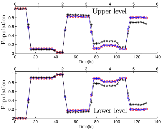
We compare the time evolution of the above mentioned observables when using the two different LZ formulas for nonadiabatic transition probabilities. In Fig. 1 we show the population of the upper and lower surfaces calculated in the deterministic setting. As suggested by our previous analysis, the curves associated with probabilities computed by the two different LZ formulas are almost indistinguishable and in good agreement with the reference. The slight deterioration of both surface hopping approximations after the third and fourth nonadiabatic passage (around time fs and fs, respectively) are due to unresolved interference effects between the upper and the lower wave packet components. This effect is also visible in Fig. 3 later on.
|
|
|
|
|

|
|
|
In Fig. 2 we show the expected position as a function of time. Ignoring nonadiabatic effects, one might expect that the average position of the wave packet follows a straight line through the conical intersection, since the initial momentum expectation equals zero, and the potential energy surfaces are radially symmetric. However, this expectation is not met, which can be explained by the surface hopping approximation: during the time interval , the wave packet is almost entirely located on the lower surface. In this case, the few trajectories on the upper surface, initially sampled from the tail of the Wigner distribution, gain relative weight with respect to the trajectories that have initiated nonadiabatic transitions. Because points sampled from the tail of the distribution are more likely to be arranged in a non symmetric way with respect to the origin in momentum space, the average momentum does not point into the direction of the conical intersection.
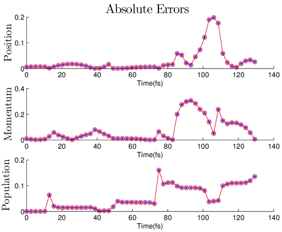
In Fig. 3 we show the absolute deviation with respect to the reference solution for the expectation values of position, momentum and population referal to the upper surface. The differences are larger when the wave function is mostly located on the lower surface namely, for the time intervals and . In particular, during the second time interval, the deviation on the three observables is amplified due to interference effects. The wave packet relative to the upper and lower surface arrive simultaneously at the conical intersection (see Fig. 2 at ). It is also important to notice that the curves describing the difference of the two Landau-Zener transition probabilities overlap quite well on the scale of the deviation with respect to the reference solution; hence, our experiments confirm the closeness of the two LZ probabilites for small values of the gap.
V.2 LZ probabilities
In Fig. 4, we analyze the difference between the LZ probabilities (3) and (4) computed simultaneously for each trajectory at each local minimum of the gap. In particular, we notice that the magnitude of the difference between the two transition probabilities is mostly or smaller and increases up to as the value of the gap function increases.
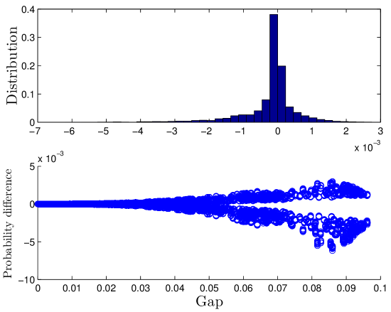
The two branches shown in the lower panel of Fig. 4 are explained by the specific form of LZ probabilities for the linear Jahn–Teller case: We have
and obtain by the calculation of section §III
| (6) |
where the plus and minus sign refer respectively to transitions from the upper level to the lower and vice versa.
In the linear Jahn–Teller situation, we have for transitions from the upper to the lower surface and for transitions from the lower to the upper surface, which explains the two branches in the lower panel.
Next we monitor individual trajectories located on the lower and the upper surface respectively. The upper panel of Fig. 5 represents the values of the two eigenvalues and along a typical upper surface trajectory. For each local minimum of we compute the transition probability in four different ways: We use the diabatic and the adiabatic formulas (3) and (4) respectively, the Jahn–Teller specific analytic version of the adiabatic formula (6) and the intermediate probability
which lacks the surface dependent term of (6). In Fig. 6, we show the corresponding information for a typical lower level trajectory.
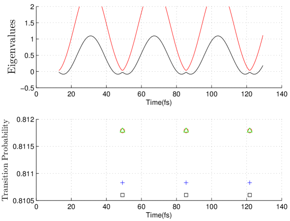
Figs. 5 and 6 depict that the differences between transition probabilities calculated by means of the different LZ formulas are small. It is worth emphasizing that these deviations are within the accuracy of the LZ approximation, since the conventional LZ formula is obtained assuming a constant and high momentum, that is, . The formulas derived in the present section for the linear Jahn-Teller case clearly show that the diabatic and the adiabatic formulas coincide in the high-energy regime, while the corrections are mainly due to an acceleration and are of the order of the energy gap.
Moreover, Figs. 5 and 6 also show that local nonadiabatic regions along classical trajectories have the form of an avoided crossing, although the global nonadiabatic region is formed by conically intersecting adiabatic energy surfaces. Since classical trajectories passing exactly through a conical intersection point are very rare, almost all local nonadiabatic regions along trajectories have the form of one-dimensional avoided crossings. The adiabatic LZ formula (4) has been applied to the one-dimensional case of several avoided crossings in atomic Na+H collisionsBelyaev and Lebedev (2011), and a good approximation of the quantum results has been found. The same is true for the diabatic formula (3), which has also been successfully applied to one-dimensional avoided crossingsFermanian-Kammerer and Lasser (2012).
The above findings are also valid for different values of the semiclassical parameter . In particular analogous distributions for the difference of are obtained when using ( mean and standard deviation being and respectively) and ( and ).
V.3 Probabilistic VS Deterministic
In this section we compare the previous results with those obtained by the probabilistic approach. The simulations presented in this section are obtained taking the average over 10 runs with the same initial trajectories used for the deterministic approach.
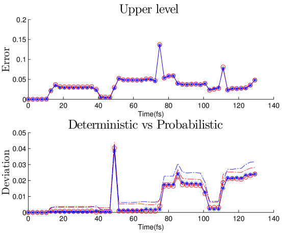
The results obtained are analogous to those displayed in the deterministic case. In particular, in the lower panel of Fig. 7 we compare the population for the upper surface obtained by the deterministic and the probabilistic approach.
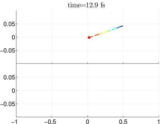
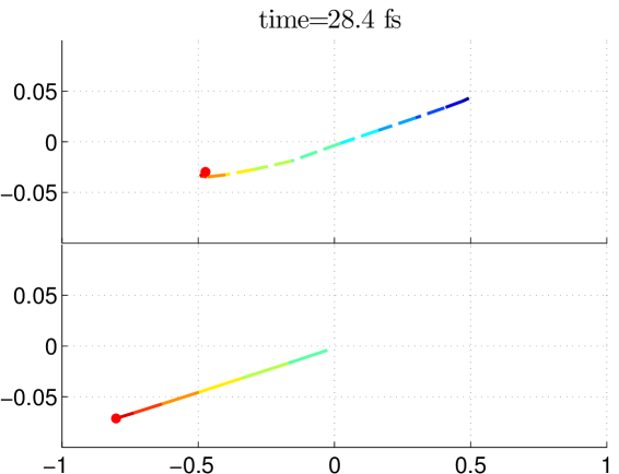
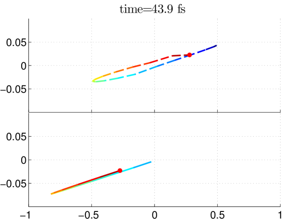
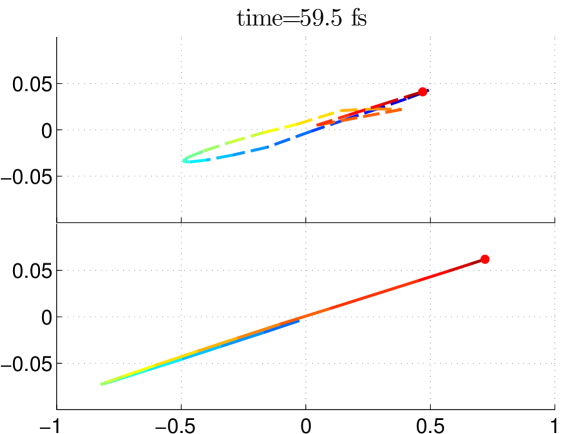
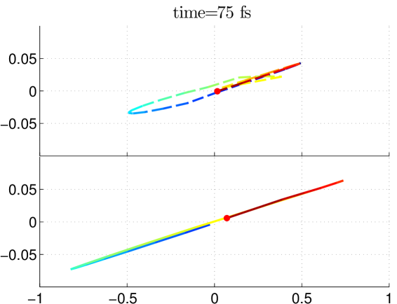
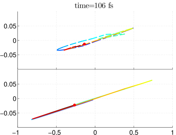
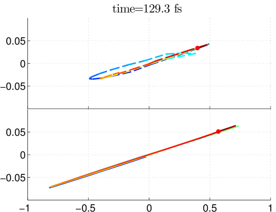
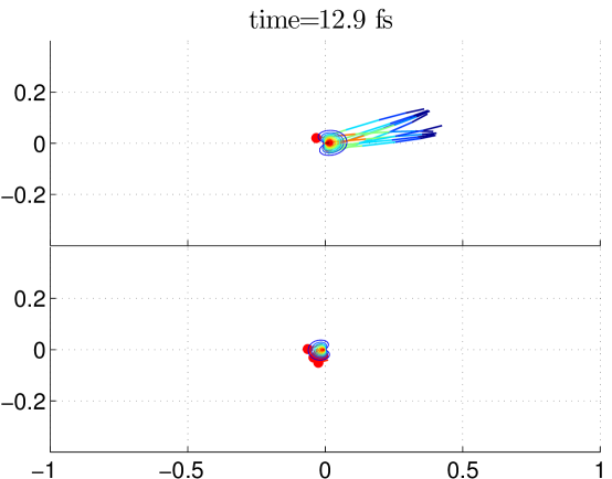
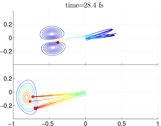
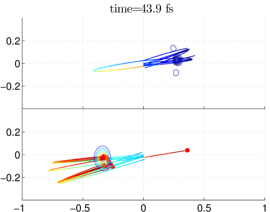
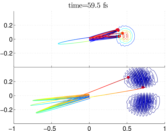
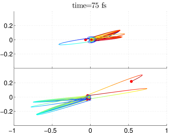
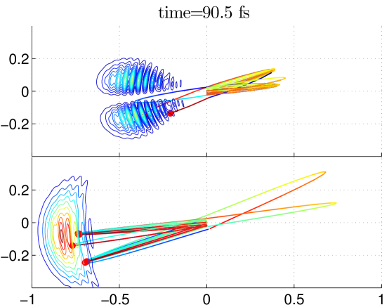
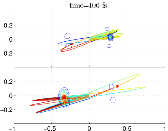
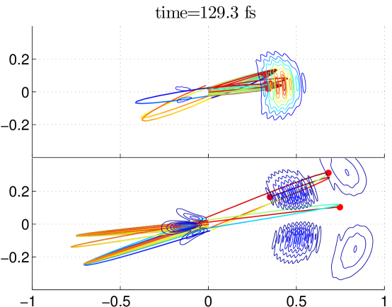
The final Fig. 8 shows the time evolution of a sample of typical surface hopping trajectories. As expected, their positions fit with the position density of the reference solution.
Comparing the deterministic and probabilistic approaches, we point out that probability currents computed by a quantum method split when passing through nonadiabatic regions, see e.g. Fig. 5 of Ref.Belyaev and Grosser (1996). The deterministic approach with its branching classical trajectories simulates this situation. Moreover, the deterministc method has been mathematically analysedFermanian-Kammerer and Lasser (2008a). On the other hand, in some cases the deterministic approach may produce too many trajectories, so that memory requirements and computing times become unfeasible and the probabilistic method with its constant number of trajectories is preferable.
VI Conclusion
We have investigated a class of surface hopping algorithms, which perform nonadiabatic transitions for each classical trajectory individually. Nonadiabatic transitions are allowed, when the surface gap attains a local minimum along an individual trajectory. We have compared two recent Landau–Zener formulas for the probability of nonadiabatic transitions, one of them requiring a diabatic representation of the potential matrix, the other one only depending on the adiabatic potential energy surfaces. Our numerical experiments confirm the expected affinity of both LZ probabilities as well as the good approximation of reference values, that have been obtained by a grid based quantum solver. We have visualized position expectations and superimposed surface hopping trajectories with reference position densities for an enhanced understanding of the effective dynamics.
Acknowledgements.
AKB gratefully acknowledges supports from the Russian Foundation for Basic Research (Grant No. 13-03-00163-a). All three authors have been supported by the German Research Foundation (DFG), Collaborative Research Center SFB-TRR 109. We thank Diane Clayton-Winter for her reading of the manuscript.
|
|
|
|
|
|
|
|
References
- Nakamura (2002) H. Nakamura, Nonadiabatic Transition: Concepts, Basic, Theories and Applications (World Scientific, Singapore, 2002).
- Domcke et al. (2004) W. Domcke, D. R. Yarkony, and H. Koeppel, eds., Conical Intersections: Electronic Structure, Dynamics and Spectroscopy (World Scientific, Singapore, 2004).
- Bersuker (2006) I. B. Bersuker, The Jahn-Teller Effect (Cambridge UP, Cambridge, 2006).
- Domcke et al. (2011) W. Domcke, D. R. Yarkony, and H. Koeppel, eds., Conical Intersections: Theory, Computation and Experiment (World Scientific, Singapore, 2011).
- Domcke and Yarkony (2012) W. Domcke and D. R. Yarkony, Annu. Rev. Phys. Chem. 63, 325 (2012).
- Tully (1998) J. C. Tully, in Modern Methods for Multidimensional Dynamics Computation in Chemistry, edited by D. L. Thompson (World Scientific, Singapore, 1998).
- Miller (1970) W. H. Miller, J. Chem. Phys. 53, 3578 (1970).
- Marcus (1972) R. A. Marcus, J. Chem. Phys. 56, 3548 (1972).
- Kreek and Marcus (1974) H. Kreek and R. A. Marcus, J. Chem. Phys. 61, 3308 (1974).
- Miller (2001) W. H. Miller, J. Phys. Chem. A 105, 2942 (2001).
- McLachlan (1964) A. D. McLachlan, Mol. Phys. 8, 39 (1964).
- Meyer and Miller (1979) H.-D. Meyer and W. H. Miller, J. Chem. Phys. 70, 3214 (1979).
- Micha (1983) D. A. Micha, J. Chem. Phys. 78, 7138 (1983).
- Kirson et al. (1984) Z. Kirson, R. B. Gerber, A. Nitzan, and M. A. Ranter, Surf. Sci. 137, 527 (1984).
- Sawada et al. (1985) S. I. Sawada, A. Nitzan, and H. Metiu, Phys. Rev. B 32, 851 (1985).
- Heller (1991) E. J. Heller, J. Chem. Phys. 94, 2723 (1991).
- Bjerre and Nikitin (1967) A. Bjerre and E. E. Nikitin, Chem. Phys. Lett. 1, 179 (1967).
- Tully and Preston (1971) J. C. Tully and R. K. Preston, J. Chem. Phys. 55, 562 (1971).
- Stine and Muckerman (1976) J. R. Stine and J. T. Muckerman, J. Chem. Phys. 65, 3975 (1976).
- Kuntz et al. (1979) P. J. Kuntz, J. Kendrick, and W. N. Whitton, Chem. Phys. 38, 147 (1979).
- Blais and Truhlar (1983) N. C. Blais and D. G. Truhlar, J. Chem. Phys. 79, 1334 (1983).
- Tully (1990) J. C. Tully, J. Chem. Phys. 93, 1061 (1990).
- Hammes-Schiffer and Tully (1994) S. Hammes-Schiffer and J. C. Tully, J. Chem. Phys. 101, 4657 (1994).
- Voronin et al. (1998) A. I. Voronin, J. M. C. Marques, and A. J. C. Varandas, J. Phys. Chem. A 102, 6057 (1998).
- Fabiano et al. (2008) E. Fabiano, G. Groenhof, and W. Thiel, Chem. Phys. 351, 111 (2008).
- Fermanian-Kammerer and Lasser (2008a) C. Fermanian-Kammerer and C. Lasser, J. Chem. Phys. 128, 144102 (2008a).
- Lasser and Swart (2008) C. Lasser and T. Swart, J. Chem. Phys. 129, 034302 (2008).
- Mueller and Stock (1997) U. Mueller and G. Stock, J. Chem. Phys. 107, 6230 (1997).
- Ben-Nun and Martinez (1998) M. Ben-Nun and T. J. Martinez, J. Chem. Phys. 108, 7244 (1998).
- Ben-Nun et al. (2000) M. Ben-Nun, J. Quenneville, and T. J. Martinez, J. Phys. Chem. A 104, 5161 (2000).
- Ben-Nun and Martinez (2002) M. Ben-Nun and T. J. Martinez, Adv. Chem. Phys. 121, 439 (2002).
- Virshup et al. (2012) A. M. Virshup, J. H. Chen, and T. J. Martinez, J. Chem. Phys. 137, 22A519 (2012).
- Tully (2012) J. C. Tully, J. Chem. Phys. 137, 22A301 (2012).
- Hagedorn (1994) G. Hagedorn, Molecular Propagation through Electron Energy Level Crossings (Amer. Math. Soc., Providence, RI, 1994).
- Hagedorn and Joye (1998) G. Hagedorn and A. Joye, Ann. Inst. H. Poincaré Phys. Théor. 68, 85 (1998).
- Fermanian-Kammerer and Gérard (2002) C. Fermanian-Kammerer and P. Gérard, Bull. Soc. Math. France 130, 123 (2002).
- Lasser and Teufel (2005) C. Lasser and S. Teufel, Comm. Pure Appl. Math. 58, 1188 (2005).
- Fermanian-Kammerer and Lasser (2008b) C. Fermanian-Kammerer and C. Lasser, SIAM J. Math. An. 40, 103 (2008b).
- Landau (1932a) L. D. Landau, Physik. Z. Sowjetunion 1, 88 (1932a).
- Landau (1932b) L. D. Landau, Physik. Z. Sowjetunion 2, 46 (1932b).
- Zener (1932) C. Zener, Proc. Roy. Soc. (London) A 137, 696 (1932).
- Miller and George (1972) W. H. Miller and T. F. George, J. Chem. Phys. 56, 5637 (1972).
- Barbatti et al. (2007) M. Barbatti, G. Granucci, M. Ruckenbauer, J. Pittner, M. Persico, and H. Lischka, NEWTON-X: a package for Newtonian dynamics close to the crossing seam. (Available at: www.newtonx.org, 2007).
- Belyaev and Lebedev (2011) A. K. Belyaev and O. V. Lebedev, Phys. Rev. A 84, 014701 (2011).
- Belyaev et al. (2010) A. K. Belyaev, P. S. Barklem, A. S. Dickinson, and F. X. Gadea, Phys. Rev. A 81, 032706 (2010).
- Belyaev (2013) A. K. Belyaev, Phys. Rev. A 88, 052704 (2013).
- Zhu and Nakamura (2001) C. Zhu and H. Nakamura, Adv. Chem. Phys. 117, 127 (2001).
- Hagedorn (1980) G. Hagedorn, Commun. Math. Phys. 77, 1 (1980).
- Spohn and Teufel (2001) H. Spohn and S. Teufel, Commun. Math. Phys. 224, 113 (2001).
- Kube et al. (2009) S. Kube, C. Lasser, and M. Weber, J. Comput. Phys. 228, 1947 (2009).
- Keller and Lasser (2013) J. Keller and C. Lasser, SIAM J. Appl. Math. 73, 1557 (2013).
- Lasser and Röblitz (2010) C. Lasser and S. Röblitz, SIAM J. Sci. Comput. 32, 1465 (2010).
- Garcia-Fernández et al. (2005) P. Garcia-Fernández, I. Bersuker, A. Aramburu, M. Barriuso, and M. Moreno, Phys. Rev. B 71, 184117 (2005).
- Fermanian-Kammerer and Lasser (2012) C. Fermanian-Kammerer and C. Lasser, J. Math. Chem. 50, 620 (2012).
- Belyaev and Grosser (1996) A. K. Belyaev and J. Grosser, J. Phys. B 29, 5843 (1996).