Generating Tatami Coverings Efficiently

Abstract.

We present two algorithms to list certain classes of monomino-domino coverings which conform to the tatami restriction; no four tiles meet. Our methods exploit structural features of tatami coverings in order to create the lists in $O(1)$ time per covering. This is faster than known methods for generating certain classes of matchings in bipartite graphs.

We discuss tatami coverings of $n\times n$ grids with $n$ monominoes and $v$ vertical dominoes, as well as tatami coverings of a two-way infinitely-wide strip of constant height, subject to the constraint that they have a finite number of non-trivial structural “features”.

These two classes are representative of two differing structural characterisations of tatami coverings which may be adapted to count other classes of tatami coverings or locally restricted matchings, such as tatami coverings of rectangles.

1. Introduction

The counting of domino coverings, together with its extension to counting perfect matchings in (planar) graphs, is a classic area of enumerative combinatorics and theoretical computer science (e.g., [11, 6, 12, 7, 8, 14]). Less attention has been paid, however, to problems where the local interactions of the dominoes are restricted in some fashion (e.g., [1]). Perhaps the most natural such restriction is the “tatami” condition, defined below. The tatami condition is quite restrictive: for example, the $10\times 13$ grid cannot be covered with dominoes and also satisfy the tatami condition. In this paper we discuss how to efficiently list certain types of tatami coverings.

Tatami mats are a traditional Japanese floor covering whose dimensions are approximately $1\textup{m}\times 1\textup{m}$ or $1\textup{m}\times 2\textup{m}$. In certain arrangements, no four tatami mats may meet. A tatami covering is a non-overlapping arrangement of $1\times 1$ monominoes, $1\times 2$ horizontal dominoes, and $2\times 1$ vertical dominoes, in which no four tiles meet. This local restriction forces a global structure which is characterised in [4] and [5].

Takeaki Uno (in [13]) generates various lists of matchings for bipartite graphs, $G=(V,E)$, with time complexities of $O(|V|)$ per matching. Our problems, which pertain to listing locally restricted matchings on grid-graphs, are $O(1)$ per matching. Specifically, we use the tatami structure to describe two classes of tatami coverings which can be generated exhaustively in constant amortised time (CAT), and discuss some general approaches to generating more complex classes of tatami coverings.

The first of these classes are the tatami coverings of the $n\times n$ grid with exactly $n$ monominoes, in a certain orientation, and $v$ vertical dominoes, denoted $\mathbf{V}(n,k)$. This is an extremal configuration of tatami covering because $n$ is the maximum possible number of monominoes in an $n\times n$ tatami covering, and it can be described with a proper subset of the general tatami structure.

Let $\mathbf{S}(n,k)$ be the subsets of $\{1,2,\ldots,n\}$ whose elements sum to $k$. Lemma 4.1 of [3] describes a bijection between the coverings in $\mathbf{V}(n,k)$ and a union of sets of the form $\mathbf{S}(a,b)\times\mathbf{S}(c,d)$ which is given in expressions (1–2).

Our technique for finding this bijection employs an operation which preserves the tatami condition, called the diagonal flip, defined in [5]. The added observation that a diagonal flip changes the orientation of the dominoes in it, enables us count the coverings classified by the number of dominoes of each orientation.

The crux of the argument uses a partition of the $n\times n$ coverings with $n$ monominoes which reveals diagonal flips each with $1,2,\ldots,k$ dominoes, respectively, that can be flipped independently. We use this to express parts of a given tatami covering as the number of subsets of $\{1,2,\ldots,n\}$ whose elements sum to $k$. An algorithm from [15] generates the $k$-sum subsets of the $n$ set in constant amortised time, and we use it to generate $\mathbf{V}(n,k)$.

The second class comprises tatami coverings of a two-way infinitely wide strip of constant height which have a finite number of non-trivial structural features (first introduced in [4]). This is a step toward generating all tatami coverings of rectangular grids by obviating the geometrical difficulties of packing the structural features into the rectangle. The algorithm itself is quite simple, arising from a system of homogeneous equations with positive coefficients, however, the equations themselves are interesting because they exert the power of the tatami structure. We contrast this with Theorem 3 of [4], which gives an algorithm for building a system of homogeneous linear recursive equations to enumerate all tatami coverings of fixed-height rectangles. Our equations, on the other hand, include the height of the strip as a parameter. We expect that our method for enumerating strip coverings of fixed-height will serve to improve methods for enumerating rectangular tatami coverings of fixed-height.

2. Tatami coverings of square regions

Let $\mathbf{T}_{n}$ be the $n\times n$ coverings which are distinct under rotation. By Corollary 2 in [4], we may assume that these have monominoes in their top corners; all others being obtained by rotation. Our goal is to generate the coverings in $\mathbf{T}_{n}$ which have exactly $k$ vertical dominoes.

Let $\mathbf{V}(n,k)$ and $\mathbf{H}(n,k)$ be the coverings in $\mathbf{T}_{n}$ with exactly $k$ vertical and horizontal dominoes, respectively, and let $\mathbf{S}(n,k)$ be the subsets of $\{1,2,\ldots,n\}$ whose elements sum to $k$. We build our exhaustive generation algorithm from the following bijection given in Lemma 4.1 of [2]:

If $n$ is even, then $|\mathbf{V}(n,k)|$ is equal to $|\mathbf{VH}(n,k)|$, which is defined as the union of the sets

(1) $$\bigcup_{i=1}^{\left\lfloor\frac{n-1}{2}\right\rfloor}\bigcup_{\begin{subarray}{c}k_{1}+k_{2}=\\ k-(n-i-1)\end{subarray}} \left(\left(\{n-i-1\}\times\mathbf{S}(n-i-2,k_{1})\right)\times\mathbf{S}(i-1,k_{2})\right.$$

$$\left.\cup\,\,\mathbf{S}(i-1,k_{2})\times\left(\{n-i-1\}\times\mathbf{S}(n-i-2,k_{1})\right)\right),$$

(2) $$\text{ and }\bigcup_{k_{1}+k_{2}=k} \mathbf{S}\left(\left\lfloor\frac{n-2}{2}\right\rfloor,k_{1}\right)\times\mathbf{S}\left(\left\lfloor\frac{n-2}{2}\right\rfloor,k_{2}\right).$$

When $n$ is odd, $|\mathbf{VH}(n,k)|$ is equal to $|\mathbf{H}(n,k)|$.

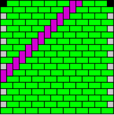
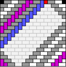
Each integer in an element of $\mathbf{VH}(n,k)$ refers to a part of the corresponding tatami covering, called a flipped diagonal. A precise definition of this is in [5], but referring to the first two coverings in Figure 1 it should be clear what a diagonal is, and what flipping it means.

Now consider the third diagram in this figure; it has four flipped diagonals. Furthermore, the largest of those flipped diagonals contains 12 vertical dominoes, there are two others with the same orientation, containing 3 and 8 vertical dominoes, and there is one with the perpendicular orientation containing 1 vertical domino. In essence, this is what (1) is counting; the outermost union is over the number of dominoes, $n-i-1$, in the largest flipped diagonal, and the inner union is over the other smaller flipped diagonals, being careful that their respective sizes adds up to the right total number of vertical dominoes $k$.

What, then, is the purpose of (2)? Note that a diagonal can flip up or down. If the largest flipped diagonal is the smaller of the two (up or down), then a different classification arises, because there is no possibility of flipped diagonals “running into” each other. This leads to the slightly simpler expression found in (2).

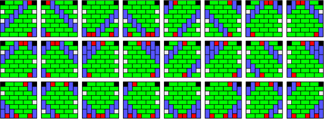
The reader is encouraged to consult Figure 2. It contains a complete listing of $\mathbf{V}(8,7)$ together with the corresponding sets. The eight pairs from (1) are listed first, followed by eight elements from (2). Note how the numbers match the number of dominoes in the various flipped diagonals.

Figure 1. From left-to-right: an unflipped diagonal is shown in magenta, the diagonal is flipped, and the tatami covering corresponding to $\mathtt{((\{12\},\{3,8\}),\{1\})}$. This is an element of $(\{n-5-1\}\times\mathbf{S}(n-5-2,11))\times\mathbf{S}(5-1,1)$, where $n=18$.

Our expression (1–2) for $\mathbf{VH}(n,k)$ can be transformed into a CAT algorithm, provided that we have a CAT algorithm for $\mathbf{S}(n,k)$. There is such a CAT algorithm, called C4 in [15]. One subtlety is that invoking C4$(n,k)$ requires $\Omega(n)$ preprocessing steps; however, there are extreme values of $k$ for which $|\mathbf{VH}(n,k)|=o(n)$. Since our goal is an algorithm that produces the (exponentially many) elements of $\mathbf{VH}(n,k)$ in constant amortised time, and which uses only $O(n)$ time in preprocessing, we will have to modify how the initialization is done.

The underlying data structure that is used by C4 is an array $\mathbf{c}=c[0],c[1],\ldots,c[n]$. In order to represent a set $\mathbf{a}=\{a_{1}<a_{2}<\cdots a_{k}\}\in\mathbf{S}(n,k)$ we set $c[0]=a_{1}$ and $c[a_{i}]=a_{i+1}$. With these rules, the array $\mathbf{c}$ is like a linked list of the elements of $\mathbf{a}$. However, the unused elements of $\mathbf{c}$ are also important, and here we set $c[i]=i+1$ for all $i\not\in\mathbf{a}$, so that the initial array corresponds to the correct values in the extreme cases.

A top level call to C4$(n,k)$ takes the array $\mathbf{c_{0}}=[n+1,2,3,\ldots,n+1]$ as input (corresponding to the empty set), an array which takes $n+1$ steps to initialise. However, when C4$(a,i)$ concludes its computation, we also have that $\mathbf{c}=\mathbf{c}_{0}$. Thus we can use most of $\mathbf{c}_{0}$ in initializing nearby successive calls to C4. In particular, we note that in (1) successive values of $n$ vary by $\pm 1$, which requires only a constant amount of change to the initialization.

Figure 2 shows the output of $\mathbf{V}(8,7)$ of the algorithm we have described.

$\mathtt{((\{6\},\{1\}),\{\})}$

$\mathtt{(\{\},(\{6\},\{1\}))}$

$\mathtt{((\{5\},\{1\}),\{1\})}$

$\mathtt{(\{1\},(\{5\},\{1\}))}$

$\mathtt{((\{5\},\{2\}),\{\})}$

$\mathtt{(\{\},(\{5\},\{2\}))}$

$\mathtt{((\{4\},\{\}),\{2,1\})}$

$\mathtt{(\{2,1\},(\{4\},\{\}))}$

$\mathtt{((\{4\},\{1\}),\{2\})}$

$\mathtt{(\{2\},(\{4\},\{1\}))}$

$\mathtt{((\{4\},\{2\}),\{1\})}$

$\mathtt{(\{1\},(\{4\},\{2\}))}$

$\mathtt{((\{4\},\{3\}),\{\})}$

$\mathtt{((\{4\},\{1,2\}),\{\})}$

$\mathtt{(\{\},(\{4\},\{3\}))}$

$\mathtt{((\{\},\{4\}),\{1,2\})}$

$\mathtt{(\{1\},\{1,2,3\})}$

$\mathtt{(\{2\},\{2,3\})}$

$\mathtt{(\{3\},\{1,3\})}$

$\mathtt{(\{1,2\},\{1,3\})}$

$\mathtt{(\{1,3\},\{3\})}$

$\mathtt{(\{1,3\},\{1,2\})}$

$\mathtt{(\{2,3\},\{2\})}$

$\mathtt{(\{1,2,3\},\{1\})}$

Figure 2. The coverings of $\mathbf{V}(8,7)$ and their representations.

Theorem 1.

There is a CAT algorithm which exhaustively generates all elements of $\mathbf{V}(n,k)$.

3. Finite tatami coverings of the infinite strip

The flipped diagonals of Section 2 are a special case of T-diagrams, given in [4, 2], which characterise monomino-domino tatami coverings of rectangles. A T-diagram is a schematic of a tatami covering, which gives a set of structural features that determine the placement of the tiles. A strip of height $r$ is a two-way infinitely wide integer grid of constant height $r$. The T-diagrams, defined for rectangular grids, also apply to the strip with the difference that there are no vertical boundaries. A finite monomino-domino tatami strip covering is a monomino-domino tatami covering of the strip with a finite number of T-diagram features. We refer to these as strip coverings, as we do not consider any other type.

Two T-diagram features are isomorphic if the respective sets of line segments they comprise are horizontal translations of each other. Two strip coverings are isomorphic if their respective features, listed from left to right, are isomorphic. See Figure 3 for an overview by example, or [2] for a detailed description.

Figure 3. A tatami covering of the strip and its T-diagram. The features, from left to right, are a vortex, a bidimer, a vee, and a loner.

Strip coverings, up to isomorphism, encapsulate some of the combinatorial properties of rectangular tatami coverings without so many of the geometric details that arise when packing feature diagrams into a rectangle. On the other hand, the T-diagram of a strip covering can be bounded by two vertical lines, thereby converting it to a rectangular T-diagram. We show that there is a CAT algorithm to generate the non-isomorphic height $r$ strip coverings with $k$-features.

Theorem 2.

If $R(r,n)$ is the number of non-isomorphic height $r$ strip coverings with exactly $n$ features, then it satisfies the system of homogeneous linear recurrence relations,

$$V_{r}(n)= 4(r-1)V_{r}(n-1)+2H_{r}(n-1),$$

$$\text{ where }V_{r}(0)=1,V_{r}(1)=4r-2;$$

$$H_{r}(n)= 2V_{r}(n-1),\text{ where }H_{r}(0)=1;$$

$$R(r,n)= V_{r}(n)+H_{r}(n).$$

Proof.

Recall that a T-diagram partitions the strip into regions, covered by vertical or horizontal bond; that is, a rotation of the basic brick-laying pattern. Let $V_{r}(n)$ and $H_{r}(n)$ be the number of non-isomorphic strip coverings whose leftmost regions are vertical and horizontal bond, respectively. The number of non-isomorphic features on the height $r$ strip are as follows:

Bidimers:

There are $r-1$ vertical, and $r-1$ possible horizontal bidimers.

Vortices:

There are $r-2$ clockwise, and $r-2$ possible counterclockwise vortices.

Vees:

There is 1 vee on the top boundary and 1 vee on the bottom.

Loners:

There are four loners, $\nearrow$, $\nwarrow$, $\searrow$, and $\swarrow$. The first two occur on the bottom boundary, and the latter on top boundary.

All of the bidimers, vortices and vees have vertical bond to their left and right. The $\searrow$ and $\nearrow$ loners have horizontal and vertical bond to their left and right, respectively, while the $\swarrow$ and $\nwarrow$ loners have vertical and horizontal bond to their left and right, respectively.

The bond coverings of the strip are either a horizontal or vertical bond. These are counted by the initial conditions $H_{r}(0)=V_{r}(0)=1$. If the leftmost region of the covering is horizontal bond, then the leftmost feature must be a $\searrow$ or $\nearrow$ loner. The region to the left of the remaining features is a vertical bond, so $H_{r}(n)=2V_{r}(n-1)$.

The total number of features with vertical bond on their left side is $(r-1)+(r-1)+(r-2)+(r-2)+1+1+1+1$, so this gives $V_{r}(1)=4r-2$. Exactly two of these features, namely $\nwarrow$ and $\swarrow$ loners, have horizontal bond on their right, so $V_{r}(n)=4(r-1)V_{r}(n-1)+2H_{r}(n-1)$.

Thus $R(r,n)=V_{r}(n)+H_{r}(n)$, as required. ∎

Corollary 1.

There exists a CAT algorithm for generating non-isomorphic, height $r$ strip coverings.

Proof.

There are $4r$ possible non-isomorphic features in height $r$ strip coverings, each of which can be expressed uniquely as an element of $\{0,1,\ldots,4r-1\}$. The recurrence relations in the proof of Theorem 2 describe a tree whose internal nodes are at least of degree $2$, and whose leaves all represent output. The recursive algorithm which naturally arises from Theorem 2, iterates through the features that can be added, given the bond of the leftmost region. After adding each feature to the covering, using its unique symbol, the algorithm recurses. There is a constant number of operations per call and a constant number of calls per leaf. Therefore the algorithm is CAT, since there are more leaves than internal nodes. ∎

Generating strip coverings with T-diagrams is a step towards doing the same for tatami coverings of rectangles. These are a natural extension of domino fixed-height coverings, proposed by Knuth in [9], and discussed in [10]. Perhaps one might proceed by considering the strip coverings whose T-diagrams are bounded on the left and right, and strip coverings with minimal distance between features. The desired respective positions for adjacent pairs of features can be tabulated in the latter case in a $4r\times 4r$ matrix.

Enumerating isomorphic strip coverings which fit in a bounded portion of the strip, perhaps is equivalent to counting a type of integer partition. That is, the total amount of space between features is a constant, while the placement of a feature can be shifted horizontally by an even number of grid squares, if it is unhindered by a neighbouring feature or a vertical boundary.

References

- [1] Ross Churchley, Jing Huang, and Xuding Zhu. Complexity of cycle transverse matching problems. In Combinatorial Algorithms (IWOCA), number 7056 in LNCS, pages 135–143. Springer Berlin / Heidelberg, January 2011.
- [2] Alejandro Erickson. Monomino-Domino Tatami Coverings. PhD thesis, University of Victoria, Canada, August 2013.
-
[3]
Alejandro Erickson and Frank Ruskey.
Enumerating maximal tatami mat coverings of square grids with
vertical dominoes.
Submitted to a journal.
http://arxiv.org/abs/1304.0070, 2013. - [4] Alejandro Erickson, Frank Ruskey, Mark Schurch, and Jennifer Woodcock. Monomer-dimer tatami tilings of rectangular regions. The Electronic Journal of Combinatorics, 18(1):24, 2011.
- [5] Alejandro Erickson and Mark Schurch. Monomer-dimer tatami tilings of square regions. Journal of Discrete Algorithms, 16(0):258–269, October 2012.
- [6] Mark Jerrum. Two-dimensional monomer-dimer systems are computationally intractable. Journal of Statistical Physics, 59(3-4):1087–1088, 1990.
- [7] P.W. Kasteleyn. The statistics of dimers on a lattice: I. the number of dimer arrangements on a quadratic lattice. Physica, 27(12):1209 – 1225, 1961.
- [8] P.W. Kasteleyn. Graph Theory and Theoretical Physics, chapter Graph theory and crystal physics. Academic Press, 1967.
- [9] Donald E. Knuth. The Art of Computer Programming, Volume 4A: Combinatorial Algorithms, Part 1. Addison-Wesley Professional, 1st edition, January 2011.
- [10] Frank Ruskey and Jennifer Woodcock. Counting fixed-height tatami tilings. The Electronic Journal of Combinatorics, 16:20, October 2009.
- [11] Richard P. Stanley. On dimer coverings of rectangles of fixed width. Discrete Applied Mathematics, 12(1):81 – 87, 1985.
- [12] H. N. V. Temperley and Michael E. Fisher. Dimer problem in statistical mechanics-an exact result. Philosophical Magazine, 6(68):1061–1063, 1961.
- [13] Takeaki Uno. Algorithms for enumerating all perfect, maximum and maximal matchings in bipartite graphs. In HonWai Leong, Hiroshi Imai, and Sanjay Jain, editors, Algorithms and Computation, volume 1350 of Lecture Notes in Computer Science, pages 92–101. Springer Berlin Heidelberg, 1997.
- [14] L. Valiant. The complexity of enumeration and reliability problems. SIAM Journal on Computing, 8(3):410–421, 1979.
- [15] Dominique Roelants van Baronaigien and Frank Ruskey. Efficient generation of subsets with a given sum. Journal of Combinatorial Mathematics and Combinatorial Computing, 14:87–96, 1993.