Conjugate Gradient Algorithm for Solving a Optimal Multiply Control Problem on
a System of Partial Differential Equations

Abstract

I development a Conjugate Gradient Method for solving a partial differential system with multiply controls. Some numerical results are depicted. Also, I present an explication of why the control over a partial differential equations system is necessary.

Keywords: Optimal Control over Partial Differential Equations; Process Engineering Methods.

1 Introduction

Given the partial differential system:

$$\left\{\begin{tabular}[]{ll}$\frac{\partial y}{\partial t}-\mu\frac{\partial^{2}y}{\partial x^{2}}+\epsilon\frac{\partial y}{\partial x}-y=0$&$\text{in }Q=\left(0,L\right)\times\left(0,T\right)$\\ $y\left(x,0\right)=y_{0},$&$t=0,$\\ $-\mu\frac{\partial y\left(0,t\right)}{\partial x}=0,$&$x=0,$\\ $\mu\frac{\partial y\left(L,t\right)}{\partial x}=0,$&$x=L.$\end{tabular}\right.$$ (S)

A conjugate gradient algorithm with several control on $\left[0,L\right]$ is developed for  S, which is similar to the Burgers’ equation.

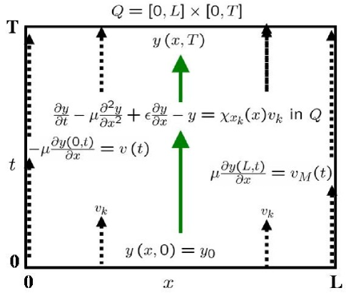
Figure 1: System (SE).

2 Several Control for  S

With an appropriate functions $v\in\mathcal{V}$, $v=(v_{0},v_{1},\ldots,v_{M})$ and $\mathcal{V}$ appropriate Hilbert Space, the system can be controlled on $x_{k}=L\frac{k}{M},$ $k=0,\ldots,M$ (see figure 1).

$$\left\{\begin{tabular}[]{ll}$\frac{\partial y}{\partial t}-\mu\frac{\partial^{2}y}{\partial x^{2}}+\epsilon\frac{\partial y}{\partial x}-y$ $=\chi_{x_{k}}(x)v_{k}$&$\text{in }Q=\left(0,L\right)\times\left(0,T\right),k=1,\ldots,M-1$\\ $y\left(x,0\right)=y_{0},$&$t=0,$\\ $-\mu\frac{\partial y\left(0,t\right)}{\partial x}=v_{0},$&$x=0,$\\ $\mu\frac{\partial y\left(L,t\right)}{\partial x}=v_{M},$&$x=L.$\end{tabular}\right.$$ (SE)

In this case, the corresponding variational control problem is

$$\left\{\begin{tabular}[]{l}Find $u^{\ast}\in\mathcal{V}$,\\ $J\left(u^{\ast}\right)\leq J\left(v\right)$, $\forall v\in\mathcal{V}$\end{tabular}\ \right.$$ (CP)

where

$$J\left(v\right)=\frac{k_{0}}{2}\sum_{k=0}^{M}\int_{0}^{T}v_{k}^{2}\text{d}t+\frac{k_{1}}{2}\iint_{Q}y^{2}\text{d}x\text{d}t+\frac{k_{2}}{2}\int_{0}^{L}y\left(x,T\right)^{2}\text{d}x$$

where $v=(v_{0},v_{1},\ldots,v_{M}),$ and $y$ is the solution of (SE) for each $v$ (see figure 1).

The equivalent form as an optimization problem is:

$$\min_{v\in\mathcal{U}}J\left(v\right)=\frac{k_{0}}{2}\sum_{k=0}^{M}\int_{0}^{T}v_{k}^{2}\text{d}t+\frac{k_{1}}{2}\iint_{Q}y^{2}\text{d}x\text{d}t+\frac{k_{2}}{2}\int_{0}^{L}y\left(x,T\right)^{2}\text{d}x,$$

where $y$ is the solution of (SE) for $v.$

In this case, the objective of the optimization problem is given a perturbation function $y_{0}$ at $t=0$ get back to the steady state to $\mathbf{0}$. Also, the controls must reduce the cost or weight of control variable $v$, keep low the cost of the evolution of the system $y\left(x,t\right).$

3 The continuous case

The continuous case is computing by a perturbation of (CP) and (SE) and using the optimal (necessary and sufficient) condition $\delta J\left(v\right)=0.$

$$\delta J\left(v\right) = k_{0}\sum_{k=0}^{M}\int_{0}^{T}v_{k}\delta v_{k}\text{d}t+k_{1}\iint_{Q}y\delta y\text{d}x\text{d}t$$

$$+ k_{2}\int_{0}^{L}y\left(x,T\right)\delta y\left(x,T\right)\text{d}x.$$

The perturbation system of the equation (SE) is

δy(x,0)=0,t=0,−μ∂δ​y​(0,t)∂x=δv0,x=0,μ∂δ​y​(L,t)∂x=δvM,x=L.\left\{\begin{tabular}[]{ll}$\frac{\partial\delta y}{\partial t}-\mu\frac{\partial^{2}\delta y}{\partial x^{2}}+\epsilon\frac{\partial\delta y}{\partial x}-\delta y=\chi_{x_{k}}(x)\delta v_{k}$&in $Q=\left(0,L\right)\times\left(0,T\right),k=1,\ldots,M-1$\\ $\delta y\left(x,0\right)=0,$&$t=0,$\\ $-\mu\frac{\partial\delta y\left(0,t\right)}{\partial x}=\delta v_{0},$&$x=0,$\\ $\mu\frac{\partial\delta y\left(L,t\right)}{\partial x}=\delta v_{M},$&$x=L.$\end{tabular}\right.

=-+-∂δy∂tμ∂2δy∂x2ϵ∂δy∂xδyχxk(x)δvkin =Q×(0,L)(0,T),=k1,…,-M1 ($\delta$SE)

Let $p\left(x,t\right)$ a sufficiently smooth function  that allow to integrate ($\delta$SE) in $Q$

$$0 = \iint_{Q}p\left(\frac{\partial\delta y}{\partial t}-\mu\frac{\partial^{2}\delta y}{\partial x^{2}}+\epsilon\frac{\partial\delta y}{\partial x}-\delta y-\chi_{x_{i}}\delta v\right)\text{d}x\text{d}t$$

$$= \iint_{Q}p\frac{\partial\delta y}{\partial t}\text{d}x\text{d}t-\mu\iint_{Q}p\frac{\partial^{2}\delta y}{\partial x^{2}}\text{d}x\text{d}t+\epsilon\iint_{Q}p\frac{\partial\delta y}{\partial x}\text{d}x\text{d}t$$

$$- \iint_{Q}p\delta y\text{d}x\text{d}t-\iint_{Q}p\chi_{x_{i}}\delta v\text{d}x\text{d}t.$$

The integration of ($\delta$SE) is achieved by the formula of integration by parts:

$$\int_{a}^{b}v\text{d}u=vu|_{a}^{b}-\int_{a}^{b}u\text{d}v.$$

Therefore

$$\iint_{Q}p\frac{\partial\delta y}{\partial t}\text{d}x\text{d}t = \int_{0}^{L}\left[\int_{0}^{T}p\frac{\partial\delta y}{\partial t}\text{d}t\right]\text{d}x~{}$$ (3.1)

$$v = p,\ \text{d}u=\frac{\partial\delta y}{\partial t}\text{d}t$$

$$= \int_{0}^{L}\left[p\left(x,T\right)\delta y\left(x,T\right)\right]_{0}^{T}\text{d}x-\iint_{Q}\frac{\partial p}{\partial t}\delta y\text{d}x\text{d}t$$

$$= \int_{0}^{L}p\left(x,T\right)\delta y\left(x,T\right)\text{d}x-\int_{0}^{L}p\left(x,0\right)\delta y\left(x,0\right)\text{d}x$$

$$- \iint_{Q}\frac{\partial p}{\partial t}\delta y\text{d}x\text{d}t$$

$$\left(\delta y\left(x,0\right)=0\right)$$

$$= \int_{0}^{L}p\left(x,T\right)\delta y\left(x,T\right)\text{d}x+\iint_{Q}\left(-\frac{\partial p}{\partial t}\right)\delta y\text{d}x\text{d}t$$

$$-\mu\iint_{Q}p\frac{\partial^{2}\delta y}{\partial x^{2}}\text{d}x\text{d}t=-\mu\int_{0}^{T}\left[\int_{0}^{L}p\frac{\partial^{2}\delta y}{\partial x^{2}}\text{d}x\right]\text{d}t~{}$$ (3.2)

$$v = p,\ \text{d}u=\frac{\partial^{2}\delta y}{\partial x^{2}}\text{d}x$$

$$= -\mu\int_{0}^{T}\left[p\left(x,t\right)\frac{\partial\delta y\left(x,t\right)}{\partial x}\right]_{0}^{L}\text{d}t+\mu\iint_{Q}\left[\frac{\partial p}{\partial x}\frac{\partial\delta y}{\partial x}\text{d}x\right]\text{d}t$$

$$v = \frac{\partial p}{\partial x},\ \text{d}u=\frac{\partial\delta y}{\partial x}\text{d}x$$

$$= \int_{0}^{T}p\left(L,t\right)\left(-\mu\frac{\partial\delta y\left(L,t\right)}{\partial x}\right)\text{d}t-\int_{0}^{T}p\left(0,t\right)\left(-\mu\frac{\partial\delta y\left(0,t\right)}{\partial x}\right)\text{d}t$$

$$+\mu\int_{0}^{T}\left[\frac{\partial p\left(x,t\right)}{\partial x}\delta y\left(x,t\right)\right]_{0}^{L}\text{d}t-\mu\iint_{Q}\frac{\partial^{2}p}{\partial x^{2}}\delta y\text{d}x\text{d}t.$$

$$\left(\mu\frac{\partial\delta y\left(L,t\right)}{\partial x}=\delta v_{M}\left(t\right),-\mu\frac{\partial\delta y\left(0,t\right)}{\partial x}=\delta v_{0}\left(t\right)\right)$$

$$= -\int_{0}^{T}p\left(L,t\right)\delta v_{M}\left(t\right)\text{d}t-\int_{0}^{T}p\left(0,t\right)\delta v_{0}\left(t\right)\text{d}t$$

$$+\mu\int_{0}^{T}\left[\frac{\partial p\left(x,t\right)}{\partial x}\delta y\left(x,t\right)\right]_{0}^{L}\text{d}t-\mu\iint_{Q}\frac{\partial^{2}p}{\partial x^{2}}\delta y\text{d}x\text{d}t$$

$$= \int_{0}^{T}p\left(L,t\right)\left(-\delta v_{M}\left(t\right)\right)\text{d}t-\int_{0}^{T}p\left(0,t\right)\delta v_{0}\left(t\right)\text{d}t$$

$$+\mu\int_{0}^{T}\frac{\partial p\left(L,t\right)}{\partial x}\delta y\left(L,t\right)\text{d}t-\mu\int_{0}^{T}\frac{\partial p\left(0,t\right)}{\partial x}\delta y\left(0,t\right)\text{d}t$$

$$-\mu\iint_{Q}\frac{\partial^{2}p}{\partial x^{2}}\delta y\text{d}x\text{d}t$$

$$= \int_{0}^{T}\left(-p\left(L,t\right)\right)\left(\delta v_{M}\left(t\right)\right)\text{d}t+\int_{0}^{T}\left(-p\left(0,t\right)\right)\delta v_{0}\left(t\right)\text{d}t$$

$$+\int_{0}^{T}\mu\frac{\partial p\left(L,t\right)}{\partial x}\delta y\left(L,t\right)\text{d}t+\int_{0}^{T}\left(-\mu\frac{\partial p\left(0,t\right)}{\partial x}\right)\delta y\left(0,t\right)\text{d}t$$

$$-\mu\iint_{Q}\frac{\partial^{2}p}{\partial x^{2}}\delta y\text{d}x\text{d}t$$

$$= \int_{0}^{T}\left(-p\left(L,t\right)\right)\left(\delta v_{M}\left(t\right)\right)\text{d}t+\int_{0}^{T}\left(-p\left(0,t\right)\right)\delta v_{0}\left(t\right)\text{d}t$$

$$+\int_{0}^{T}\mu\frac{\partial p\left(L,t\right)}{\partial x}\delta y\left(L,t\right)\text{d}t+\int_{0}^{T}\left(-\mu\frac{\partial p\left(0,t\right)}{\partial x}\right)\delta y\left(0,t\right)\text{d}t$$

$$+\iint_{Q}\left(-\mu\frac{\partial^{2}p}{\partial x^{2}}\right)\delta y\text{d}x\text{d}t$$

$$\epsilon\iint_{Q}p\frac{\partial\delta y}{\partial x}\text{d}x\text{d}t = \epsilon\int_{0}^{T}\left[\int_{0}^{L}p\frac{\partial\delta y}{\partial x}\text{d}x\right]\text{d}t~{}$$ (3.3)

$$v = p,\ \text{d}u=\frac{\partial\delta y}{\partial x}\text{d}x$$

$$= \epsilon\int_{0}^{T}\left[p\left(x,t\right)\delta y\left(x,t\right)\right]_{0}^{L}\text{d}t-\epsilon\iint_{Q}\frac{\partial p}{\partial x}\delta y\text{d}x\text{d}t$$

$$= \epsilon\int_{0}^{T}p\left(L,t\right)\delta y\left(L,t\right)\text{d}t-\epsilon\int_{0}^{T}p\left(0,t\right)\delta y\left(0,t\right)\text{d}t$$

$$-\epsilon\iint_{Q}\frac{\partial p}{\partial x}\delta y\text{d}x\text{d}t$$

$$= \int_{0}^{T}\epsilon p\left(L,t\right)\delta y\left(L,t\right)\text{d}t+\int_{0}^{T}\left(-\epsilon p\left(0,t\right)\right)\delta y\left(0,t\right)\text{d}t$$

$$-\epsilon\iint_{Q}\frac{\partial p}{\partial x}\delta y\text{d}x\text{d}t$$

$$-\iint_{Q}p\delta y\text{d}x\text{d}t=\iint_{Q}\left(-p\right)\delta y\text{d}x\text{d}t.~{}$$ (3.4)

$$-\iint_{Q}p\chi_{x_{i}}\delta v\text{d}x\text{d}t = \sum_{i=1}^{M-1}\int_{0}^{T}\left(-p_{i}\right)\delta v_{i}\text{d}t~{}$$ (3.5)

$$\text{where }\chi_{x_{i}}p = p_{i}.~{}$$

$$0 = (\ref{1})+(\ref{2})+(\ref{3})+(\ref{4})+(\ref{5})$$

$$= \int_{0}^{L}p\left(x,T\right)\delta y\left(x,T\right)\text{d}x+\iint_{Q}\left(-\frac{\partial p}{\partial t}\right)\delta y\text{d}x\text{d}t$$

$$+\int_{0}^{T}\left(-p\left(L,t\right)\right)\left(\delta v_{M}\left(t\right)\right)\text{d}t+\int_{0}^{T}\left(-p\left(0,t\right)\right)\delta v_{0}\left(t\right)\text{d}t+\int_{0}^{T}\mu\frac{\partial p\left(L,t\right)}{\partial x}\delta y\left(L,t\right)\text{d}t$$

$$+\int_{0}^{T}\left(-\mu\frac{\partial p\left(0,t\right)}{\partial x}\right)\delta y\left(0,t\right)\text{d}t+\iint_{Q}\left(-\mu\frac{\partial^{2}p}{\partial x^{2}}\right)\delta y\text{d}x\text{d}t$$

$$+\int_{0}^{T}\epsilon p\left(L,t\right)\delta y\left(L,t\right)\text{d}t+\int_{0}^{T}\left(-\in p\left(0,t\right)\right)\delta y\left(0,t\right)\text{d}t-\epsilon\iint_{Q}\frac{\partial p}{\partial x}\delta y\text{d}x\text{d}t$$

$$+\iint_{Q}\left(-p\right)\delta y\text{d}x\text{d}t$$

$$+\sum_{i=1}^{M-1}\int_{0}^{T}\left(-p_{i}\right)\delta v_{i}\text{d}t$$

$$= \sum_{i=0}^{M}\int_{0}^{T}\left(-p_{i}\right)\delta v_{i}\text{d}t$$

$$+\iint_{Q}\left(-\frac{\partial p}{\partial t}-\mu\frac{\partial^{2}p}{\partial x^{2}}-\epsilon\frac{\partial p}{\partial x}-p\right)\delta y\text{d}x\text{d}t$$

$$+\int_{0}^{L}p\left(x,T\right)\delta y\left(x,T\right)\text{d}x$$

$$+\int_{0}^{T}\left(\mu\frac{\partial p\left(L,t\right)}{\partial x}+\epsilon p\left(L,t\right)\right)\delta y\left(L,t\right)\text{d}t+\int_{0}^{T}\left(-\mu\frac{\partial p\left(0,t\right)}{\partial x}-\epsilon p\left(0,t\right)\right)\delta y\left(0,t\right)\text{d}t$$

Adjusting terms with

$$\delta J\left(v\right)=k_{0}\sum_{k=0}^{M}\int_{0}^{T}v_{k}\delta v_{k}\text{d}t+k_{1}\iint_{Q}y\delta y\text{d}x\text{d}t+k_{2}\int_{0}^{L}y\left(x,T\right)\delta y\left(x,T\right)\text{d}x,$$

the adjoint system is

$$\left\{\begin{tabular}[]{ll}$p\left(x,T\right)=k_{2}y\left(x,T\right)$,&$x\in\left[0,L\right]$\\ $\mu\frac{\partial p}{\partial x}\left(L,t\right)+\epsilon p\left(L,t\right)=0$,&$t\in\left[0,T\right]$\\ $\mu\frac{\partial p}{\partial x}\left(0,t\right)+\epsilon p\left(0,t\right)=0$&$t\in\left[0,T\right]$\\ $\frac{\partial p}{\partial t}+\mu\frac{\partial^{2}p}{\partial x^{2}}+\epsilon\frac{\partial p}{\partial x}+p=-k_{1}y,$&in $Q$\end{tabular}\ \right. \delta$$ (ASE)

also

$$\nabla J\left(v\right)=k_{0}\sum_{k=0}^{M}\left(v_{k}-p_{k}\left(x,t\right)\right).$$

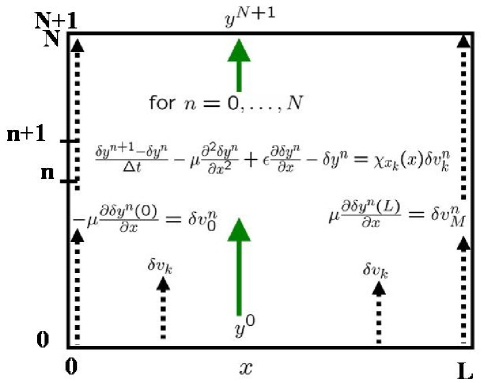
Figure 2: Discretization on time of ($\delta$SE^Δt).

4 Discretization on Time

The discretization on time of $J^{{}^{{\Delta t}}}\left(v\right)$ is

$$J^{{}^{{\Delta t}}}\left(v\right)=\frac{{\Delta t}}{2}\sum_{k=0}^{M}\sum_{n=0}^{N}\left\|v_{k}^{n}\right\|^{2}+\frac{k_{1}{\Delta t}}{2}\sum_{n=0}^{N}\int_{0}^{L}\left\|y^{n}\right\|^{2}\text{d}x+\frac{k_{2}}{2}\int_{0}^{L}\left\|y^{N+1}\left(x\right)\right\|^{2}\text{d}x$$

where $N>0$,and ${\Delta t}=\frac{T}{N}$.

Now, the forward discretization on time of (SE) is

yn+1−ynΔ​t−μ∂2yn∂x2+ϵ∂yn∂x−yn=χxk(x)vkn,−μ∂yn​(0)∂x=v0n,μ∂yn​(L)∂x=vMn.\left\{\begin{tabular}[]{l}$y^{0}=y_{0}.$\\ for $n=0,\ldots,N$\\ $\frac{y^{n+1}-y^{n}}{{\Delta t}}-\mu\frac{\partial^{2}y^{n}}{\partial x^{2}}+\epsilon\frac{\partial y^{n}}{\partial x}-y^{n}=\chi_{x_{k}}(x)v_{k}^{n},$\\ $-\mu\frac{\partial y^{n}\left(0\right)}{\partial x}=v_{0}^{n},$\\ $\mu\frac{\partial y^{n}\left(L\right)}{\partial x}=v_{M}^{n}.$\end{tabular}\ \right.

$$\{\begin{array}{c}\end{array}$$=y0y0.for =n0,…,N (SE^△t)

The optimal condition is

$$\delta J^{{\Delta t}}(v)=\sum_{k=0}^{M}\left(\nabla J^{{}^{{\Delta t}}}\left(v_{k}\right),\delta v_{k}\right)_{\mathcal{U}^{{\Delta t}}}=0.$$

And

$$\delta J^{{\Delta t}}(v)=k_{0}\Delta t\sum_{k=0}^{M}\sum_{n=0}^{N}v_{k}^{n}\delta v_{k}^{n}+k_{1}{\Delta t}\sum_{n=0}^{N}\int_{0}^{L}y^{n}\delta y^{n}\text{d}x+k_{2}\int_{0}^{L}y^{N+1}\delta y^{N+1}\text{d}x.$$

By the other hand, the perturbation of (SE^△t) is

δ​yn+1−δ​ynΔ​t−μ∂2δ​yn∂x2+ϵ∂δ​yn∂x−δyn=χxk(x)δvkn,−μ∂δ​yn​(0)∂x=δv0n,μ∂δ​yn​(L)∂x=δvMn.\left\{\begin{tabular}[]{l}$\delta y^{0}=0.$\\ for $n=0,\ldots,N$\\ $\frac{\delta y^{n+1}-\delta y^{n}}{{\Delta t}}-\mu\frac{\partial^{2}\delta y^{n}}{\partial x^{2}}+\epsilon\frac{\partial\delta y^{n}}{\partial x}-\delta y^{n}=\chi_{x_{k}}(x)\delta v_{k}^{n},$\\ $-\mu\frac{\partial\delta y^{n}\left(0\right)}{\partial x}=\delta v_{0}^{n},$\\ $\mu\frac{\partial\delta y^{n}\left(L\right)}{\partial x}=\delta v_{M}^{n}.$\end{tabular}\ \right.

$$\{\begin{array}{c}\end{array}$$=δy00.for =n0,…,N ($\delta$SE^Δt)

Figure 2 depicts ($\delta$SE^Δt).

Now, multiplying these by appropriate functions $p^{n}$ to integrate:

$${\Delta t}\sum_{n=0}^{N}\int_{0}^{L}p^{n}\left(\frac{\delta y^{n+1}-\delta y^{n}}{{\Delta t}}-\mu\frac{\partial^{2}\delta y^{n}}{\partial x^{2}}+\epsilon\frac{\partial\delta y^{n}}{\partial x}-\delta y^{n}-\chi_{x_{k}}\delta v_{k}^{n}\right)\text{d}x=0.$$

$${\Delta t}\sum_{n=0}^{N}\int_{0}^{L}p^{n}\left(\frac{\delta y^{n+1}-\delta y^{n}}{{\Delta t}}\right)\text{d}x=$$ (4.1)

$$= -\int_{0}^{L}p^{0}\frac{\delta y^{0}}{{\Delta t}}\text{d}x-{\Delta t}\sum_{n=1}^{N}\int_{0}^{L}\left(\frac{p^{n}-p^{n-1}}{{\Delta t}}\right)\delta y^{n}\text{d}x+\int_{0}^{L}p^{N}\delta y^{N+1}\text{d}x$$

$$-{\Delta t}\sum_{n=1}^{N}\int_{0}^{L}\left(\frac{p^{n}-p^{n-1}}{{\Delta t}}\right)\delta y^{n}\text{d}x+\int_{0}^{L}p^{N}\delta y^{N+1}\text{d}x.$$

$${\Delta t}\sum_{n=0}^{N}\int_{0}^{L}p^{n}\left(-\mu\frac{\partial^{2}\delta y^{n}}{\partial x^{2}}\right)\text{d}x=~{}$$ (4.2)

$$= {\Delta t}\sum_{n=0}^{N}p\left[-\mu\frac{\partial\delta y}{\partial x}\right]_{0}^{L}+\mu{\Delta t}\sum_{n=0}^{N}\frac{\partial p}{\partial x}\left[\delta y\right]_{0}^{L}-\mu{\Delta t}\sum_{n=0}^{N}\int_{0}^{L}\frac{\partial^{2}p}{\partial x^{2}}\delta y\text{d}x$$

$$= -{\Delta t}\sum_{n=0}^{N}p^{n}\left(0\right)\left(\delta v^{n}\right)+\mu{\Delta t}\sum_{n=0}^{N}\frac{\partial p^{n}\left(L\right)}{\partial x}\delta y\left(L\right)$$

$$-\mu{\Delta t}\sum_{n=0}^{N}\int_{0}^{L}\frac{\partial^{2}p}{\partial x^{2}}\delta y\text{d}x.$$

$${\Delta t}\sum_{n=0}^{N}\int_{0}^{L}p^{n}\left(\epsilon\frac{\partial\delta y^{n}}{\partial x}\right)\text{d}x=\epsilon\sum_{n=0}^{N}p^{n}\left(L\right)\delta y\left(L\right)-\epsilon\sum_{n=0}^{N}\int_{0}^{L}\frac{\partial p}{\partial x}\delta y\text{d}x.$$ (4.3)

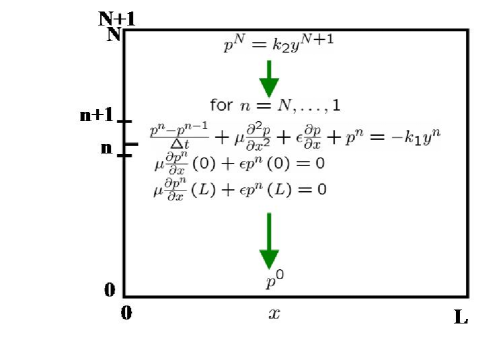
Figure 3: Discretization on time of adjoint system of (SE).

$${\Delta t}\sum_{n=0}^{N}\int_{0}^{L}p^{n}\left(-\delta y^{n}\right)\text{d}x.$$ (4.4)

$$0=(\ref{6})+(\ref{7})+(\ref{8})+(\ref{9})=$$

$${\Delta t}\sum_{n=1}^{N}\int_{0}^{L}\left(-\frac{p^{n}-p^{n-1}}{{\Delta t}}-\mu\frac{\partial^{2}p}{\partial x^{2}}-\epsilon\frac{\partial p}{\partial x}-p^{n}\right)\delta y^{n}\text{d}x+\int_{0}^{L}p^{N}\delta y^{N+1}\text{d}x$$

$$-{\Delta t}\sum_{n=0}^{N}p\left(0\right)\left(\delta v^{n}\right)+\mu{\Delta t}\sum_{n=0}^{N}\frac{\partial p^{n}}{\partial x}\left(L\right)\delta y\left(L\right)+\epsilon\sum_{n=0}^{N}p\left(L\right)\delta y\left(L\right).$$

Therefore the discretization on time of the adjoint system (see figure 3) is

pn−pn−1Δ​t+μ∂2p∂x2+ϵ∂p∂x+pn=−k1yn,μ∂pn∂x(0)+ϵpn(0)=0μ∂pn∂x(L)+ϵpn(L)=0.\left\{\begin{tabular}[]{l}$p^{N}=k_{2}y^{N+1}.$\\ for $n=N,\ldots,1$\\ $\frac{p^{n}-p^{n-1}}{{\Delta t}}+\mu\frac{\partial^{2}p}{\partial x^{2}}+\epsilon\frac{\partial p}{\partial x}+p^{n}=-k_{1}y^{n},$\\ $\mu\frac{\partial p^{n}}{\partial x}\left(0\right)+\epsilon p^{n}\left(0\right)=0$\\ $\mu\frac{\partial p^{n}}{\partial x}\left(L\right)+\epsilon p^{n}\left(L\right)=0$.\end{tabular}\ \right.

$$\{\begin{array}{c}\end{array}$$=pNk2y+N1.for =nN,…,1 (ASE^Δt)

And

$$\nabla J^{{}^{{\Delta t}}}\left(v\right)=\sum_{k=0}^{M}\left\{v_{k}^{n}-p^{n}\left(0\right)\right\}_{n=0}^{N}.$$

4.1 Fully discretization

Let $H>0,$ $H$ is an integer multiple of $M$, and $\bigtriangleup x={h}=\frac{L}{H}$. The indices for axis $x$ are $-1\leq j\leq H+1$. Note that two sets of points are added on $j=-1$, and $j=H+1$, this is convenient because the frontier conditions on $x=0$ ($-\mu\frac{\partial y\left(0,t\right)}{\partial x}=v\left(t\right),$) and $x=L$ ($\mu\frac{\partial y\left(L,t\right)}{\partial x}=0$) can be inserted before and after the points of interest $0$ to $H$ on $x$.

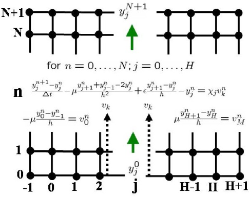
Figure 4: Fully discretization of (SE).

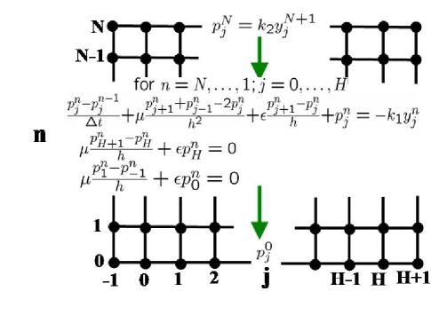
Figure 5: Fully discretization of adjoint system of (SE).

The corresponding fully discrete steady equations (see figure 4)are

yjn+1−yjnΔ​t−μyj+1n+yj−1n−2​yjnh2+ϵyj+1n−yjnh−yjn=χxjvk−μy0n−y−1nh=v0nμyH+1n−yHnh=vMn.\left\{\begin{tabular}[]{l}$y_{j}^{0}=y_{0,j}$, $j=0,\ldots,H$\\ for $n=0,\ldots,N$, $j=0,\ldots,H$\\ $\frac{y_{j}^{n+1}-y_{j}^{n}}{{\Delta t}}-\mu\frac{y_{j+1}^{n}+y_{j-1}^{n}-2y_{j}^{n}}{h^{2}}+\epsilon\frac{y_{j+1}^{n}-y_{j}^{n}}{h}-y_{j}^{n}=\chi_{x_{j}}v_{k}$\\ $-\mu\frac{y_{0}^{n}-y_{-1}^{n}}{h}=v_{0}^{n}$\\ $\mu\frac{y_{H+1}^{n}-y_{H}^{n}}{h}=v_{M}^{n}.$\end{tabular}\ \right.

$$\{\begin{array}{c}\end{array}$$ =yj0y0,j, =j0,…,H for =n0,…,N, =j0,…,H (SE${}_{\vartriangle x}^{\vartriangle t}$)

$-\mu\frac{y_{0}^{n}-y_{-1}^{n}}{h}=v_{0}^{n}$

$-\mu y_{0}^{n}+\mu y_{-1}^{n}=hv_{0}^{n}$

$+y_{-1}^{n}=\left(hv_{0}^{n}+\mu y_{0}^{n}\right)/\mu$

$+y_{-1}^{n}=\frac{h}{\mu}v_{0}^{n}+y_{0}^{n}$

$\mu\frac{y_{H+1}^{n}-y_{H}^{n}}{h}=v_{M}^{n}$

$\mu\left(y_{H+1}^{n}-y_{H}^{n}\right)=hv_{M}^{n}$

$\mu y_{H+1}^{n}-\mu y_{H}^{n}=hv_{M}^{n}$

$\mu y_{H+1}^{n}=\mu y_{H}^{n}+hv_{M}^{n}$

$y_{H+1}^{n}=y_{H}^{n}+\frac{h}{\mu}v_{M}^{n}$

The adjoint equations (see figure 5) are

pjn−pjn−1Δ​t+μpj+1n+pj−1n−2​pjnh2+ϵpj+1n−pjnh+pjn=−k1yjnμpH+1n−pHnh+ϵpHn=0.μp0n−p−1nh+ϵp−1n=0\left\{\begin{tabular}[]{l}$p_{j}^{N}=k_{2}y_{j}^{N+1}$, $j=0,\ldots,H$\\ for $n=N,\ldots,1$, $j=0,\ldots,H$\\ $\frac{p_{j}^{n}-p_{j}^{n-1}}{{\Delta t}}+\mu\frac{p_{j+1}^{n}+p_{j-1}^{n}-2p_{j}^{n}}{h^{2}}+\epsilon\frac{p_{j+1}^{n}-p_{j}^{n}}{h}+p_{j}^{n}=-k_{1}y_{j}^{n}$\\ $\mu\frac{p_{H+1}^{n}-p_{H}^{n}}{h}+\epsilon p_{H}^{n}=0.$\\ $\mu\frac{p_{0}^{n}-p_{-1}^{n}}{h}+\epsilon p_{-1}^{n}=0$\end{tabular}\right.

$$\{\begin{array}{c}\end{array}$$ =pjNk2yj+N1, =j0,…,H for =nN,…,1, =j0,…,H (ASE${}_{\bigtriangleup x}^{\bigtriangleup t}$)

$\frac{p_{j}^{n}-p_{j}^{n-1}}{{\Delta t}}+\mu\frac{p_{j+1}^{n}+p_{j-1}^{n}-2p_{j}^{n}}{h^{2}}+\epsilon\frac{p_{j+1}^{n}-p_{j}^{n}}{h}+p_{j}^{n}=-k_{1}y_{j}^{n}$.

The solution is $p_{j}^{n-1}=\frac{h^{2}p_{j}^{n}+\mu\Delta tp_{j+1}^{n}+\mu\Delta tp_{j-1}^{n}-2\mu\Delta tp_{j}^{n}+\epsilon\Delta thp_{j+1}^{n}-\epsilon\Delta thp_{j}^{n}+p_{j}^{n}\Delta th^{2}+k_{1}y_{j}^{n}\Delta th^{2}}{h^{2}}=$

$p_{j}^{n-1}=p_{j}^{n}+\frac{\mu\Delta tp_{j+1}^{n}+\mu\Delta tp_{j-1}^{n}-2\mu\Delta tp_{j}^{n}+\epsilon\Delta thp_{j+1}^{n}-\epsilon\Delta thp_{j}^{n}+p_{j}^{n}\Delta th^{2}}{h^{2}}+k_{1}y_{j}^{n}\Delta t=$

$p_{j}^{n-1}=p_{j}^{n}+\frac{\mu\Delta t\left(p_{j+1}^{n}+p_{j-1}^{n}-2p_{j}^{n}\right)}{h^{2}}+\frac{\epsilon\Delta t\left(p_{j+1}^{n}-hp_{j}^{n}\right)}{h}+p_{j}^{n}\Delta t+k_{1}y_{j}^{n}\Delta t=$

$\mu\frac{p_{0}^{n}-p_{-1}^{n}}{h}+\epsilon p_{-1}^{n}=0$

$\frac{\mu}{h}p_{0}^{n}-\frac{\mu}{h}p_{-1}^{n}+\epsilon p_{-1}^{n}=0$

$\mu p_{0}^{n}-\mu p_{-1}^{n}+\epsilon hp_{-1}^{n}=0$

$p_{-1}^{n}=\mu p_{0}^{n}/\left(\mu-\epsilon h\right)$

$\mu\frac{p_{H+1}^{n}-p_{H}^{n}}{h}+\epsilon p_{H}^{n}=0$

$\mu p_{H+1}^{n}-\mu p_{H}^{n}=-\epsilon hp_{H}^{n}$

$\mu p_{H+1}^{n}=\left(\mu-\epsilon\right)p_{H}^{n}/\mu.$

And the corresponding perturbation equations are

δ​yjn+1−δ​yjnΔ​t−μδ​yj+1n+δ​yj−1n−2​δ​yjnh2+ϵδ​yj+1n−δ​yjnh−δyjn=χxjδvkn−μδ​y0n−δ​y−1nh=δv0n,μδ​yH+1n−δ​yHnh=δvMn.\left\{\begin{tabular}[]{l}$\delta y_{j}^{0}=0$, $j=0,\ldots,H$\\ for $n=0,\ldots,N$, $j=0,\ldots,H$\\ $\frac{\delta y_{j}^{n+1}-\delta y_{j}^{n}}{{\Delta t}}-\mu\frac{\delta y_{j+1}^{n}+\delta y_{j-1}^{n}-2\delta y_{j}^{n}}{h^{2}}+\epsilon\frac{\delta y_{j+1}^{n}-\delta y_{j}^{n}}{h}-\delta y_{j}^{n}=\chi_{x_{j}}\delta v_{k}^{n}$\\ $-\mu\frac{\delta y_{0}^{n}-\delta y_{-1}^{n}}{h}=\delta v_{0}^{n},$\\ $\mu\frac{\delta y_{H+1}^{n}-\delta y_{H}^{n}}{h}=\delta v_{M}^{n}.$\end{tabular}\ \right.

$$\{\begin{array}{c}\end{array}$$ =δyj00, =j0,…,H for =n0,…,N, =j0,…,H ($\delta$SE${}_{\bigtriangleup x}^{\bigtriangleup t}$)

The corresponding variational control problem is

$$\left\{\begin{tabular}[]{l}Find $u^{\ast}=\left\{u^{n}\right\}\in\mathcal{V}_{\bigtriangleup x}^{\bigtriangleup t}(=\mathbb{R}^{N\times M}$)\\ $J_{\bigtriangleup x}^{\bigtriangleup t}\left(u^{\ast}\right)\leq J_{\bigtriangleup x}^{\bigtriangleup t}\left(v\right)\text{, }\forall\,v\in\mathcal{V}_{\bigtriangleup x}^{\bigtriangleup t}$\end{tabular}\ \right. {}_{\bigtriangleup x}^{\bigtriangleup t}$$ (CP)

where

$$J_{\bigtriangleup x}^{\bigtriangleup t}\left(v\right)=\frac{{\Delta t}}{2}\sum_{k=0}^{M}\sum_{n=0}^{N}\left[v_{k}^{n}\right]^{2}+\frac{k_{1}{\Delta th}}{2}\sum_{n=0}^{N}\sum_{j=0}^{H}\left[y_{j}^{n}\right]^{2}+\frac{k_{2}h}{2}\sum_{j=0}^{H}\left[y_{j}^{N+1}\right]^{2},$$

and $y=\left\{y_{j}^{n}\right\}_{-1\leq j\leq H+1}^{0\leq n\leq N+1}$ is the solution of (SE${}_{\vartriangle x}^{\vartriangle t}$) with $v$. Note that $H\geq M$ and $H$ must be a multiple of $M$ in order to have $\chi_{x_{j}}\delta v_{k}^{n}=\delta v_{k}^{n},\forall k=0,\ldots,M.$

5 The Conjugate Gradient Algorithm

The CG algorithm for the fully discrete control problem (CP${}_{\bigtriangleup x}^{\bigtriangleup t}$) is:

1. Given $\varepsilon$ (the tolerance to stop the algorithm), $0<\varepsilon\ll 1$, and $\ \left\{u^{n,0}\right\}=\mathbf{0}\in$ $\mathcal{V}_{\bigtriangleup x}^{\bigtriangleup t}.$

2. Solve the equation (SE${}_{\vartriangle x}^{\vartriangle t}$), and

   with the solution $\left\{y_{j}^{n,0}\right\}_{-1\leq j\leq H+1}^{0\leq n\leq N+1}$ solve (ASE${}_{\bigtriangleup x}^{\bigtriangleup t}$) to get $\left\{p_{j}^{n,0}\right\}_{-1\leq j\leq H+1}^{0\leq n\leq N}.$

3. Compute $g^{0}=\left\{u_{j_{k}}^{n,0}+p_{j_{k}}^{n,0}\right\}_{0\leq j_{k}\leq H}^{0\leq n\leq N}$, and set $w^{0}=g^{0}$.

   Now, we have $u^{m}$, $g^{m}$, and $w^{m}$.

4. If $\frac{\left(g^{m+1},g^{m+1}\right)_{\mathcal{V}}}{\left(g^{0},g^{0}\right)_{\mathcal{V}}}<\epsilon^{2}$ take $u^{m+1}$ as the solution and stop.

5. Compute $m=m+1$.

6. Solve the equation ($\delta$SE${}_{\bigtriangleup x}^{\bigtriangleup t}$), and

   with the solution $\overline{y}=\left\{\delta y_{j}^{n,m}\right\}_{-1\leq j\leq H+1}^{0\leq n\leq N+1}$ solve (ASE${}_{\bigtriangleup x}^{\bigtriangleup t}$) to get $\overline{p}=\left\{p_{j}^{n,m}\right\}_{-1\leq j\leq H+1}^{0\leq n\leq N}.$

7. Compute $\overline{g}^{m}=\left\{w_{j_{k}}^{n,m}+\overline{p}_{j_{k}}^{n,m}\right\}_{0\leq j_{k}\leq H}^{0\leq n\leq N}$, $\rho^{m}=\left(g^{m},g^{m}\right)_{\mathcal{V}}$, $u^{m+1}=u^{m}-\rho^{m}w^{m}$, and $g^{m+1}=g^{m}-\rho^{m}\overline{g}^{m}.$

8. If $\frac{\left(g^{m+1},g^{m+1}\right)_{\mathcal{V}}}{\left(g^{0},g^{0}\right)_{\mathcal{V}}}<\epsilon^{2}$ take $u^{m+1}$ as the solution and stop.

9. Compute $\gamma^{m}=\frac{\left(g^{m+1},g^{m+1}\right)_{\mathcal{V}}}{\left(g^{m},g^{m}\right)_{\mathcal{V}}}$, and $w^{m+1}=g^{m+1}+\gamma^{m}w^{m}$

10. Go to step 5.

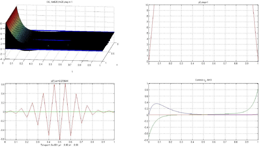
Figure 6: $y_{0}$ is a positive pulse, 3 controls.

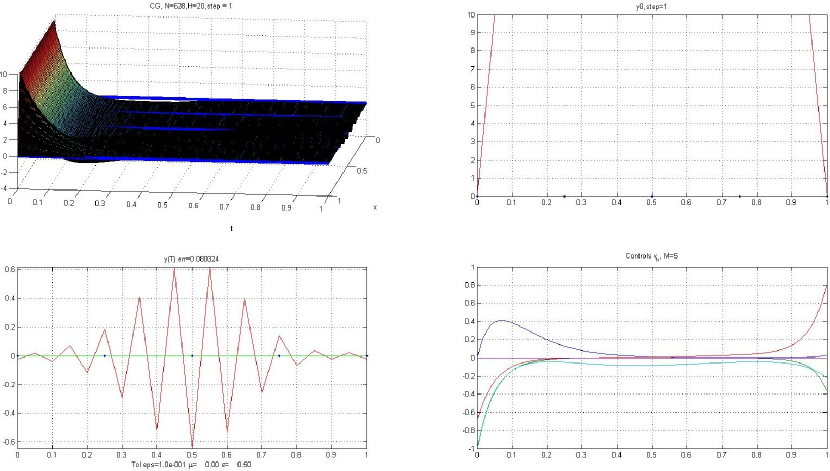
Figure 7: $y_{0}$ is a positive pulse, 5 controls.

Figure 8: $y_{0}$ is a positive pulse, 11 controls.

6 Numerical Experiments

A program of the Conjugated Gradient Method (Section 5) was development in Matlab.

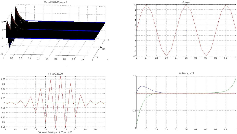
Figure 9: $y_{0}$ $=$ $10\sin(5\pi x),$ 3 controls.

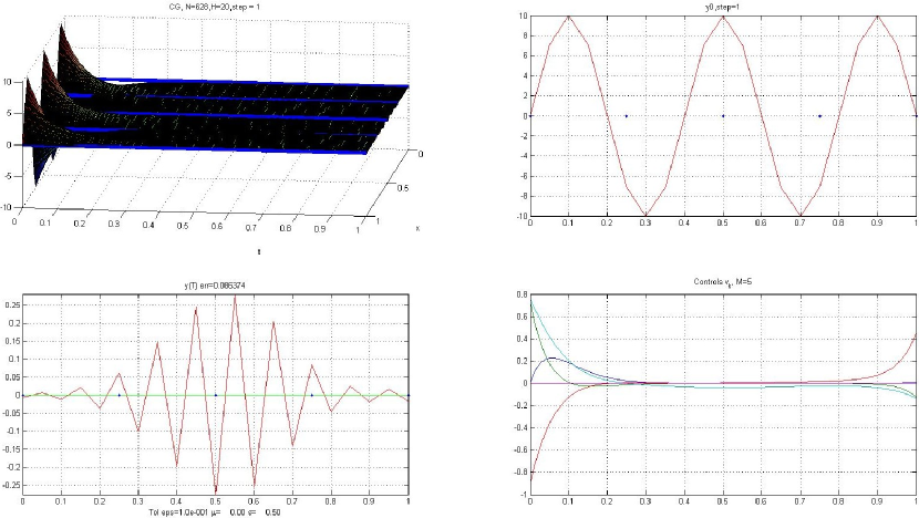
Figure 10: $y_{0}$ $=$ $10\sin(5\pi x),$ 5 controls.

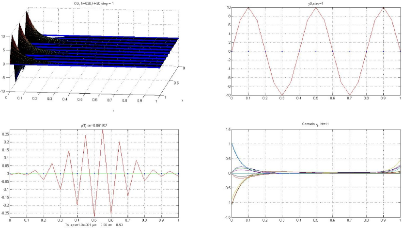
Figure 11: $y_{0}$ $=$ $10\sin(5\pi x),$ 11 controls.

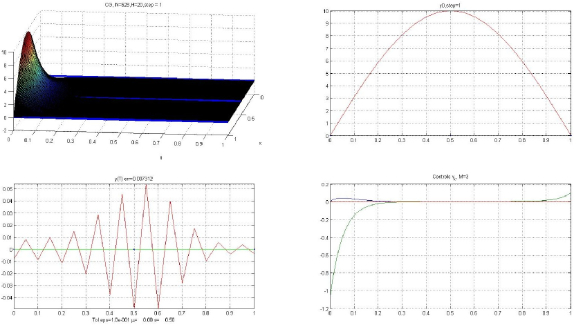
Figure 12: $y_{0}$ $=$ $10\sin(\pi x),$ 3 controls.

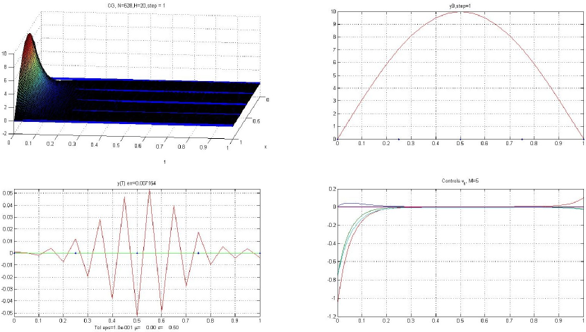
Figure 13: $y_{0}$ $=$ $10\sin(\pi x),$ 5 controls.

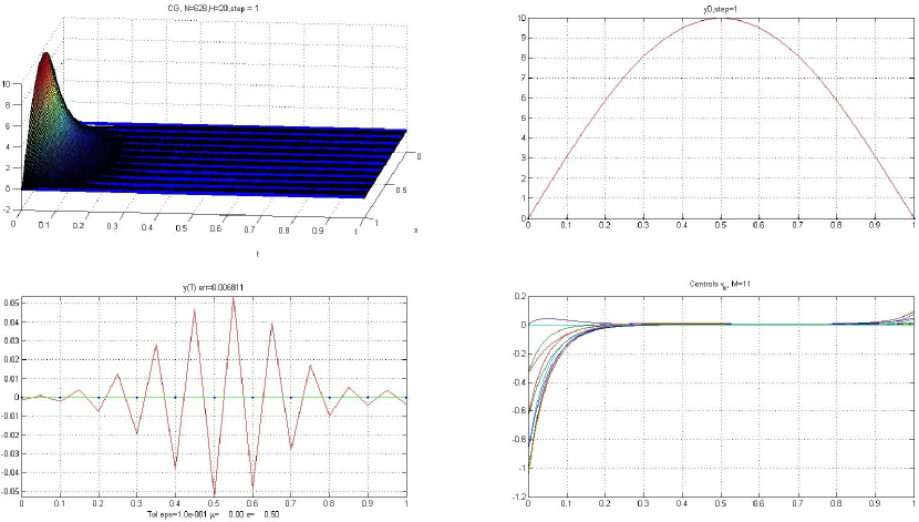
Figure 14: $y_{0}$ $=$ $10\sin(\pi x),$ 11 controls.

Three numerical experiments were designed:

1. $y_{0}$ is a positive pulse in $[0,1].$

2. $y_{0}$ $=$ $10\sin(5\pi x),$ $x\in[0,1].$

3. $y_{0}$ $=$ $10\sin(\pi x),$ $x\in[0,1].$

The results are depicted in figures  6,  7,  8,  9,  10,  11,  12,  13, and  14. Each figure depicts the evolution of the state $y$, the initial state $y_{0}$, the final state $y(T)$, and the graphs of the controls. These experiments depict:

1. The graphs of the controls show that the cost increases with the numbers of controls.

2. The graphs of the controls show that the controls behave different.

3. It seems that with more controls the final state is closed to steady state $\mathbf{0}$. However, there is a dependency of the initial state $y_{0}$ and the numbers of controls in the contrary. Figures 6,  7, and  8 depict a case where 3 controls behave better than 11 controls.

4. It seems that with more controls the evolution of the $y$ is controlled. In all cases, the controls are enough to diminish the initial state $y_{0}$ and to keep under control the evolution of the system over time.

7 Motivation for controlling

We preferred to leave this section at the end, because these notes are principally aimed for graduate students, which could be interested in developing their own simulators. It is possibly, that they already know the importance of the Theory of Control on Systems over Partial Differential Equations or the control for industrial process.

From the abundant literature, we mention the book of partial differential equations [4], and for Control the books [1, 3]. These notes were developed from the talk in [2].

The following problem depicts a classical problem for a parabolic equation with three physical-chemical components.

1. Advection. It is the scalar variation at each point of a vector field, by example, the contaminant entrainment in a medium.

2. Reaction. It is the response or reaction of the system, by example, the heat exchanges in a system.

3. Diffusion. It is the gradient (change or transport) of system components.

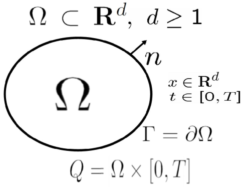
Figure 15: Sistem’s domain

Let be the following parabolic equation where the advection is $V\cdot\nabla\varphi$, the reaction is $f\left(\varphi\right)$, and the diffusion is $\nabla\cdot\left(A\nabla\varphi\right)$ acting over the time. It is Equation of the State System.

$$\begin{tabular}[]{l}$\frac{\partial\varphi}{\partial t}-\nabla\cdot\left(A\nabla\varphi\right)+V\cdot\nabla\varphi+f\left(\varphi\right)=0\text{ en }Q=\Omega\times\left[0,T\right],$\\ $A\nabla\varphi\cdot n=0\text{ en }\Sigma=\Gamma\times\left[0,T\right],$\\ $\varphi\left(x,0\right)=\varphi_{0}\left(x\right)\text{ }x\in\Omega$\end{tabular}~{}.~{}$$ (SEE)

where $\Omega\subset\mathbf{R}^{d}$ ($d\geq 1$, dimension) it is a smooth region, with orientated boundary $\Gamma=\partial\Omega$, $n$ represents a normal unit vector on $\Gamma$ (pointing outside of $\Omega$), $T>0$ is the time ( including the possiblity $T=\infty)$. Figure 15 depicts (SEE).

The intern product $\cdot$ is the usual, $a,b\in\mathbf{R}^{d},a\cdot b=\sum\limits_{i=1}^{d}a_{i}b_{i}$, $A$ is a real tensor function (diffusion matrix), $V:\Omega\rightarrow\mathbf{R}^{d}$ is a vectorial function, $f:\mathbf{R}\rightarrow\mathbf{R}$ is a real function, and $\varphi(x,t)$ is the phenomena function that occurs in $Q.$

In addition we assume that:

$$A(x)\xi\cdot\xi\geq\alpha\left|\xi\right|^{2},\forall\xi\in\mathbf{R}^{d}\text{ for almost all }x\in\Omega$$

which means that $A$ is uniformly positive definite for almost all $x$ in $\Omega.$

For the vector function $V,$ we assume:

$$\nabla\cdot V = 0\text{ (divergence free)}$$

$$\frac{\partial V}{\partial t} = 0\text{ (it is constant over time)}$$

$$V\cdot n = 0\text{ on }\Gamma$$

Control is necessary for this System, let be a reaction function given by

$$f\left(\varphi\right)=C-\lambda e^{\varphi}$$

where $C,\lambda>0$ are real positive constants.

Then the steady state solution for such $f$  fulfill:

$$\frac{\partial\varphi}{\partial t}+f\left(\varphi\right)=0$$ (7.1)

and it is given by

$$\varphi_{s}=\frac{\ln C}{\lambda}$$

Note that $\varphi_{s}$ is constant,so that the equation (7.1), substituting $\varphi_{s}$ is fulfill (because $f\left(\varphi_{s}\right)=C-\lambda e^{\varphi_{s}}=C-\lambda e^{\frac{\ln C}{\lambda}}=0)$.

Assuming that for some $t>0$, the system was its stable steady state solution $\varphi=\varphi_{s}$.

Now, $\varphi=\varphi_{s}$ at some time $t_{0}=0$ has a small constant perturbation $\delta\varphi,$ independent from $x$ y $t$ (with $\nabla\delta\varphi=0$ y $\frac{\partial\delta\varphi}{\partial t}=0$).

For this perturbation, the system evolves under the following ordinary differential equation:

$$\frac{\text{d}\varphi}{\text{d}t} = \lambda e^{\varphi}-C\text{, }\lambda,C>0,\text{ real constants}$$

$$\varphi\left(0\right) = \varphi_{s}+\delta\varphi$$

This model behaves with a constant positive perturbation, $\delta\varphi>0$, such that $\varphi\rightarrow+\infty.$ By other hand, if the perturbation is a constant negative, $\delta\varphi<0$, then $\varphi_{t\rightarrow\infty}\rightarrow-\infty$. In the following paragraphs, it is showed that in the former the deviation from the stable state grows fast to $+\infty$, and in the second case the deviation of the stable state is slow and steady toward $-\infty$ as the time progress.

This means that around a stable steady state solution, the introduction a small constant perturbation makes the system unstable. To verify the above statement, we proceed by the Euler Method to numerically integrate the above equation:

$$\frac{\text{d}\varphi}{\text{d}t} = \lambda e^{\varphi}-C\text{, }\lambda,C>0,\text{ real constants}$$

$$\varphi\left(0\right) = \frac{\ln C}{\lambda}+\delta\varphi$$

Without loss of generality we take $\triangle t=1$, $C=1,\lambda=1,\delta\varphi=0.1>0,$ and approach $\frac{d\varphi}{dt}$ by a time difference between $n$ and $n-1$.

The resulting approximation difference equation is

$\varphi_{n}=\exp\left(\varphi_{n-1}\right)+\varphi_{n-1}-1.$

From the initial condition:

$\varphi_{0}=\frac{\ln C}{\lambda}+\delta\varphi=0.1$

The numerical estimations are

$\varphi_{1}=\exp\left(0.1\right)+0.1-1=\allowbreak 0.205\,17$

$\varphi_{2}=\exp\left(0.205\,17\right)+0.205\,17-1\allowbreak=$ $0.432\,9$

$\varphi_{3}=\exp\left(0.432\,9\right)+0.432\,9-1=\allowbreak 0.974\,64$

$\varphi_{4}=\exp\left(0.974\,64\right)+0.974\,64-1=\allowbreak 2.\,\allowbreak 624\,8$

$\varphi_{5}=\exp\left(2.\,\allowbreak 624\,8\right)+2.\,\allowbreak 624\,8-1=\allowbreak 15.\,\allowbreak 427$

$\varphi_{6}=\exp\left(15.\,\allowbreak 427\right)+15.\,\allowbreak 427-1=\allowbreak 5.\,\allowbreak 010\,3\times 10^{6}$

$\varphi_{7}=\exp\left(5.\,\allowbreak 010\,3\times 10^{6}\right)+5.\,\allowbreak 010\,3\times 10^{6}-1=\allowbreak 4.\,\allowbreak 392\,2\times 10^{2175945}$

$\varphi\left(t\right)$ in a finite time grows very quickly, it tends accelerated to $\infty.$

By other hand, assuming that $\delta\varphi=-0.1<0$, and using the same constants $C$ y $\lambda$, the numerical estimations for this case are

$\varphi_{0}=-0.1$

$\varphi_{1}=\exp\left(-0.1\right)+\left(-0.1\right)-1=\allowbreak-0.195\,16$

$\varphi_{2}=\exp\left(-0.195\,16\right)+\left(-0.195\,16\right)-1=\allowbreak-0.372\,46$

$\varphi_{3}=\exp\left(-0.372\,46\right)+\left(-0.372\,46\right)-1=\allowbreak-0.683\,42$

$\varphi_{4}=\exp\left(-0.683\,42\right)+\left(-0.683\,42\right)-1=\allowbreak-1.\,\allowbreak 178\,5$

$\varphi_{5}=\exp\left(-1.\,\allowbreak 178\,5\right)+\left(-1.\,\allowbreak 178\,5\right)-1=\allowbreak-1.\,\allowbreak 870\,8$

$\varphi_{6}=\exp\left(-1.\,\allowbreak 870\,8\right)+\left(-1.\,\allowbreak 870\,8\right)-1=\allowbreak-2.\,\allowbreak 716\,8$

$\varphi_{7}=\exp\left(-2.\,\allowbreak 716\,8\right)+\left(-2.\,\allowbreak 716\,8\right)-1=\allowbreak-3.\,\allowbreak 650\,7$

$\varphi_{8}=\exp\left(-3.\,\allowbreak 650\,7\right)+\left(-3.\,\allowbreak 650\,7\right)-1=\allowbreak-4.\,\allowbreak 624\,7$

$\varphi_{9}=\exp\left(-4.\,\allowbreak 624\,7\right)+\left(-4.\,\allowbreak 624\,7\right)-1=\allowbreak-5.\,\allowbreak 614\,9$

$\varphi_{10}=\exp\left(-5.\,\allowbreak 614\,9\right)+-5.\,\allowbreak 614\,9-1=\allowbreak-6.\,\allowbreak 611\,3$

$\varphi_{11}=\exp\left(-6.\,\allowbreak 611\,3\right)+-6.\,\allowbreak 611\,3-1=\allowbreak-7.\,\allowbreak 610\,0$

$\varphi\left(t\right)$ is decreasing slowly to $-\infty.$

The previous numerical results clearly depicts that a control is necessary to prevent such behavior and to return the system to the steady state solution $\varphi_{s}$.

Conclusions and future work

I did not expect implying that more controls means best result. The numerical results depict this but the positive pulse. However, in all numerical experiments the controls push back the controlled system SE to the steady solution $\mathbf{0}$. As in global optimization, the objective functions and problems have a relation or compromise within the solution and the method for solving them. Here, there are different behaviors between initial state and numbers of controls.

The position of controls could be interesting to study in the future.

My students of the master program in Engineering Process help me to obtain preliminary results in less than three months. They study the relation between one control and the initial state, they found examples where one control does not work. Also, they want to known about how difficult could be to apply advance mathematics and to development control process software. I already have the one control version, so they did the preliminary experiments. I promise them, that I will development the multiple controls version. My teaching philosophy is to help people to understand and to be free of myths. Of course it is difficult but, it is better to development a toy simulator than to buy one.

I believe, that is a good practice to help the students and people to understand and take advance mathematics and to build by themselves software, as an open box.

References

- [1] R. Glowinski. Numerical Methods for Nonlinear Variational Problems. Computational Physics. Springer-Verlag, 1984.
- [2] R. Glowinski. A Brief Introduction on the Optimal Control of Partial Differential Equations. Workshop en Métodos Numéricos de Optimización y de Control Optimo en PDE, Guanajuato, Gto., México, 2006.
- [3] R. Glowinski, J. L. Lions, and J. He. Exact and Approximate Controllability for Distributed Parameter Systems. Encyclopedia of Mathematics. Cambrigde University Press, 2008.
- [4] K. W. Morton and D. F. Mayers. Numerical Solution of Partial Differential Equations. Cambrigde University Press, 1994.