A fast directional boundary element method for high frequency acoustic problems in three dimensions

Abstract

A highly efficient fast boundary element method (BEM) for solving large-scale engineering acoustic problems in a broad frequency range is developed and implemented. The acoustic problems are modeled by the Burton-Miller boundary integral equation (BIE), thus the fictitious frequency issue is completely avoided. The BIE is discretized by using the collocation method with piecewise constant elements. The linear systems are solved iteratively and accelerated by using a newly developed kernel-independent wideband fast directional algorithm (FDA) for fast summation of oscillatory kernels. In addition, the computational efficiency of the FDA is further promoted by exploiting the low-rank features of the translation matrices. The high accuracy and nearly linear computational complexity of the present method are clearly demonstrated by typical examples. An acoustic scattering problem with dimensionless wave number $kD$ (where $k$ is the wave number and $D$ is the typical length of the obstacle) up to 1000 and the degrees of freedom up to 4 million is successfully solved within 4 hours on a computer with one core and the memory usage is 24.7 GB.

1 Introduction

Acoustic wave propagation is a commonly studied problem for its wide application in noise controls, ultrasonic diagnostics, sonar imaging, etc. One of the most popular solving approaches is boundary element method due to its unique advantages, such as dimension reduction, high accuracy and suitability for infinite domain cases. The conventional boundary element method leads to dense system matrix. As a result, the computational complexity is at least of order $O(N^{2})$, which makes it prohibitive for large-scale problems.

In the past three decades, many fast algorithms have been proposed to circumvent this disadvantage. A group of these algorithms make use of the asymptotic smooth property of the kernel function when the field points are far away from the source points. As a result, the large submatrices of the system matrix corresponding to far-field interactions are of numerically low rank. These algorithms are performed on an octree (quadtree for two dimensional cases), which is constructed by subdividing the integral region recursively. By applying low rank approximations hierarchically on the octree, the computational complexity can be reduced to $O(N)$. The low rank decomposition of the submatrices can be generated by various methods, resulting in diverse algorithms, including fast multipole method (FMM)[1, 2, 3], $\mathcal{H}$-matrix method[4], panel clustering method[5], ACA[6, 7], wavelet compression method[8, 9] etc. However, it is found that these low-rank approximating algorithms are only suitable for low frequency problems, since the ranks of the submatrices tend to be proportional to their sizes, leading to $O(N^{2})$ complexity for high frequency problems.

Another class of these fast algorithms make use of the translational invariant property of the kernel function. By mapping the information on the elements onto Cartesian grids, then diagonalizing the matrix by Fast Fourier Transformation[10, 11], the required operations can be reduced significantly. It can be very efficient for both low and high frequency problems, but its computational complexity is $O(N^{4/3}\log N)$ when applied in accelerating BEM[12, 13]. Besides, it is well known that the performance of the FFT-based algorithms deteriorates in the cases with highly nonuniform mesh discretization.

Using the diagonal forms of the translation operators in FMM makes it possible to obtain $O(N\log N)$ complexity for high frequency problems[14]. Later the wideband FMM[15, 16] is developed which successfully avoids its numerical instability at low frequencies by combining it with the traditional FMM. In wideband FMM, the octree is divided into high frequency regime and low frequency regime according to the size of the cubes in each level. Different translation methods are applied in these regimes, i.e., in the low frequency regime, the translations are performed in the same way as in traditional FMM; while far field signature and diagonal forms of the translation operators are used in the high frequency regime. It is stable, accurate and efficient for both low and high frequency problems. However, it requires analytical expansions of the kernel, thus the translations are very complicated and the algorithm is kernel-dependent. This poses a severe limitation on its applications.

Fast directional algorithm is another efficient algorithm for solving high frequency problems[17, 18], by which the computational complexity can also be reduced to $O(N\log N)$. It is a FMM-like algorithm which takes the advantage of the directional low rank property of the kernel function to do the translations in the high frequency regime. Consequently, the low rank approximation are applied in both the low and high frequency regimes, the only difference is the definition of the interaction list. Various low rank approximating techniques can be used, resulting in variants of the fast directional algorithm[18, 19, 20].

In this paper, the fast directional algorithm based on equivalent densities is adapted to accelerate the 3D acoustic BEM for the first time, and a modified version of a recently developed M2L translations accelerating technique named as SArcmp is applied to improve its efficiency. The advantages of this algorithm lies in the following two aspects. First, no analytical expansions for the kernel function is required, thus the algorithm is completely kernel-independent and easy to implement. Second, integrals with different layer kernel functions can be accelerated by the same process, thus it is very convenient to handle Burton-Miller formulation in which four layer kernel functions are included. In this sense, it is more suitable to accelerated acoustic problems than other fast algorithm.

2 Boundary integral formulation for acoustic problems

Consider the acoustic problems described by Helmholtz equation

$$\nabla^{2}u(\bm{x})+k^{2}u(\bm{x})=0,\quad\bm{x}\in\Omega,$$ (1)

where $u$ is the velocity potential, $k=\omega/c$ is the wavenumber, and $\Omega$ is the acoustic field domain. The acoustic field can be solved by conventional boundary integral equation

$$c(\bm{x})u(\bm{x})+\int_{\Gamma}\frac{\partial G(\bm{x},\bm{y})}{\partial\bm{n}(\bm{y})}u(\bm{y})\mathrm{d}\bm{y}=\int_{\Gamma}G(\bm{x},\bm{y})\frac{\partial u(\bm{y})}{\partial\bm{n}(\bm{y})}\mathrm{d}\bm{y}+u^{\text{inc}}(\bm{x}),\quad\bm{x}\in\Gamma,$$ (2)

where $\Gamma=\partial\Omega$ is the boundary of the acoustic field, $c(\bm{x})$ is the solid angle at $\bm{x}$, and $G(\bm{x},\bm{y})$ is the fundamental solution

$$G(\bm{x},\bm{y})=\frac{e^{ikr}}{4\pi r},\quad r=|\bm{x}-\bm{y}|.$$ (3)

However, it is well known that it fails to yield unique solutions at the characteristic frequencies. One of the most widely used methods to overcome this problem is the Burton-Miller formulation, which is generated by combining (2) and its normal derivatives

$$\begin{split}c(\bm{x})u(\bm{x})+\int_{\Gamma}\frac{\partial G(\bm{x},\bm{y})}{\partial\bm{n}(\bm{y})}u(\bm{y})\mathrm{d}\bm{y}+\alpha\int_{\Gamma}\frac{\partial^{2}G(\bm{x},\bm{y})}{\partial\bm{n}(\bm{x})\partial\bm{n}(\bm{y})}u(\bm{y})\mathrm{d}\bm{y}\\ =-\alpha c(\bm{x})\frac{\partial u(\bm{x})}{\partial\bm{n}(\bm{x})}+\int_{\Gamma}G(\bm{x},\bm{y})\frac{\partial u(\bm{y})}{\partial\bm{n}(\bm{y})}\mathrm{d}\bm{y}+\alpha\int_{\Gamma}\frac{\partial G(\bm{x},\bm{y})}{\partial\bm{n}(\bm{x})}\frac{\partial u(\bm{y})}{\partial\bm{n}(\bm{y})}\mathrm{d}\bm{y}\\ +u^{\text{inc}}(\bm{x})+\alpha\frac{\partial u^{\text{inc}}(\bm{x})}{\partial\bm{n}(\bm{x})},\quad\bm{x}\in\Gamma,\end{split}$$ (4)

where $\alpha$ is the combining factor that is suggested to be chosen as $i/k$[21].

By discretizing (4) with basis functions $\chi(\bm{x})$ and weight functions $w(\bm{x})$, the integrals would be transformed into summations. Take the left hand side for example, it can be discretized into

$$\begin{split}p_{i}=&\sum_{j=1}^{N}\int_{\Gamma_{i}}w_{i}(\bm{x})\int_{\Gamma_{j}}\left[\frac{\partial G(\bm{x},\bm{y})}{\partial\bm{n}(\bm{y})}+\alpha\frac{\partial^{2}G(\bm{x},\bm{y})}{\partial\bm{n}(\bm{x}_{i})\partial\bm{n}(\bm{y})}\right]q_{j}\chi_{j}(\bm{y})\mathrm{d}\bm{y}\mathrm{d}\bm{x}\\ =&\int_{\Gamma_{i}}w_{i}(\bm{x})\left[1+\alpha\frac{\partial}{\partial\bm{n}(\bm{x})}\right]\left[\sum_{j=1}^{N}\int_{\Gamma_{j}}\frac{\partial G(\bm{x},\bm{y})}{\partial\bm{n}(\bm{y})}\chi_{j}(\bm{y})\mathrm{d}\bm{y}\cdot q_{j}\right]\mathrm{d}\bm{x},\\ &\quad i=1,2,\dots,N,\end{split}$$ (5)

where $\Gamma_{i}$ and $\Gamma_{j}$ is the supporting region of the $i$-th weight function $w_{i}(\bm{x})$ and the $j$-th basis function $\chi_{j}(\bm{y})$, respectively, and $q_{j}$ is the coefficient for $\chi_{j}(\bm{y})$. Evaluating the summation directly requires $O(N^{2})$ operators. In the next section, we will discuss how to accelerate the evaluation by fast directional algorithm.

3 Fast directional algorithm for Burton-Miller formulation

The key of fast directional algorithm is the construction of the fast potential evaluating scheme using the directional low rank property of the kernel function. In this section, the fast evaluating scheme is also based on equivalent densities and check potentials as [17, 18]. However, the equivalent points and check points are defined as the quadrature points instead of defined by pseudo skeleton approach, resulting in a simpler fast directional algorithm.

3.1 Directional low rank approximation

Suppose $X$ and $Y$ be the target point set and the source point set, respectively. When $X$ and $Y$ satisfy the directional parabolic separation condition, as shown in Figure 1, the kernel function can be approximated by

$$\left|G(\bm{x},\bm{y})-\sum_{i=1}^{T(\varepsilon)}\alpha_{i}(\bm{x})\beta_{i}(\bm{y})\right|<\varepsilon,$$ (6)

where $T(\varepsilon)$ has an upper bound that is independent of $k$ and $w$. In this case, the evaluation for the potentials on $X$ can be accelerated via equivalent densities and check potentials.

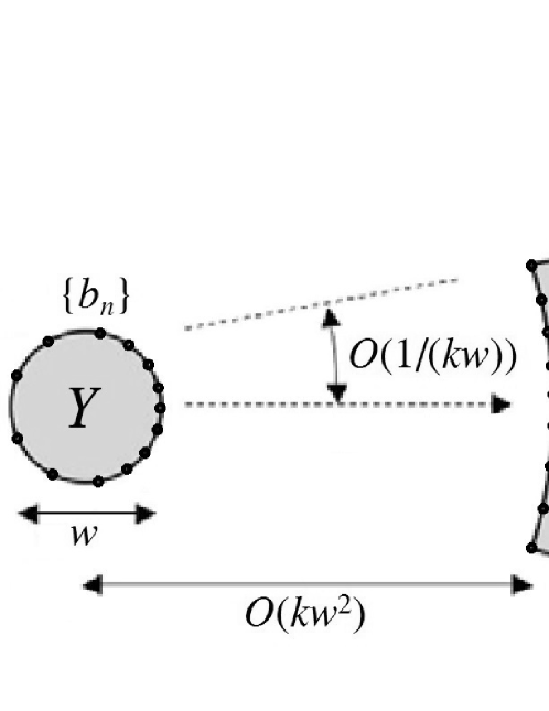
Figure 1: Source set $Y$ and target set $X$ satisfying the directional parabolic separation condition.

First we find certain distributions of monopole sources $\sigma(\bm{y})$ on directional outgoing equivalent surface $\bm{y}^{Y,\text{o}}$, that can reproduce the potential field $p(\bm{x})$ in $X$ excited by arbitrary source densities $q(\bm{y})$ in $Y$. Similar with the kernel independent FMM[22], the equivalent surface $\bm{y}^{Y,\text{o}}$ need to enclose $Y$ in order to guarantee the existence of the directional outgoing equivalent densities $\sigma(\bm{y})$; and a check surface $\bm{x}^{Y,\text{o}}$ enclosing $X$ can be defined, such that once the $\sigma(\bm{y})$ can reproduce the potential field on $\bm{x}^{Y,\text{o}}$, it can excite the same potential field inside $X$. Therefore, the directional outgoing equivalent densities $\sigma(\bm{y})$ on $\bm{y}^{Y,\text{o}}$ can be computed by the following equation

$$\int_{\bm{y}^{Y,\text{o}}}G(\bm{x},\bm{y})\sigma(\bm{y})\mathrm{d}\bm{y}=p^{Y,\text{o}}(\bm{x}),\quad\bm{x}\in\bm{x}^{y,\text{o}}.$$ (7)

where $p^{Y,\text{o}}(\bm{x})$ is calculated by the original source densities $q(\bm{y})$ in $Y$. For point sources, $p^{Y,\text{o}}(\bm{x})$ is evaluated by summation; while for distributed sources, it should be evaluated by quadrature. Equation (7) can be viewed as a transformation from $\sigma(\bm{y})$ to $p^{Y,\text{o}}(\bm{x})$, and the transformation is of rank $T(\varepsilon)$. Therefore, it can be discretized by Nyström method using $O(T(\varepsilon))$ directional outgoing equivalent points $\bm{y}$’s and $O(T(\varepsilon))$ directional outgoing check points $\bm{x}$’s, i.e.,

$$p^{Y,\text{o}}(\bm{x}_{i})=\int_{Y}G(\bm{x}_{i},\bm{y})\sigma(\bm{y})\mathrm{d}\bm{y}=\sum_{j}w_{j}G(\bm{x}_{i},\bm{y}_{j})\sigma(\bm{y}_{j}),\quad\bm{x}_{i}\in\bm{x}^{Y,\text{o}},\bm{y}_{j}\in\bm{y}^{Y,\text{o}}.$$ (8)

This suggests that we can take distribute monopole source densities $q^{Y,\text{o}}(\bm{y}_{j})=w_{j}\sigma(\bm{y}_{j})$ at quadrature points as the directional outgoing equivalent densities, and the transformation from directional outgoing equivalent densities to directional outgoing check potentials becomes

$$p^{Y,\text{o}}(\bm{x}_{i})=\sum_{j}G(\bm{x}_{i},\bm{y}_{j})q^{Y,\text{o}}(\bm{y}_{j}),\quad\bm{x}_{i}\in\bm{x}^{Y,\text{o}},\bm{y}_{j}\in\bm{y}^{Y,\text{o}}.$$ (9)

In our algorithm, the directional outgoing equivalent points are distributed in the same way as the non-directional outgoing equivalent points in [22, 23], that is, they are distributed on a cube surface with $p$ points in each direction. The directional outgoing check points are defined by mapping the points onto the surface of the directional cone which is bounded by the size of the boundary $\Gamma$, and are focused at the smaller end, as illustrated in Figure 2(a).

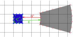
(a) S2M

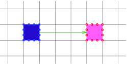
(b) M2L

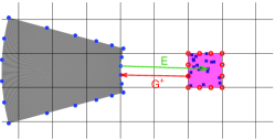
(c) L2T

Figure 2: Single level fast directional summation for $N$-body problems.

When the roles of $X$ and $Y$ are reversed, i.e., the potentials in $Y$ produced by sources inside $X$ need to be evaluated, the directional incoming equivalent densities $q^{X,\text{i}}(\bm{y})$ on the directional incoming equivalent points $\bm{y}^{X,\text{i}}$ can be constructed in the same manner via the directional incoming check potentials $p^{X,\text{i}}(\bm{x})$ on the directional incoming check points $\bm{x}^{X,\text{i}}$.

Since the kernel is rotational invariant, the directional equivalent points and the directional check points for other directional cones can be obtained by rotation, and the matrices translating the check potentials into equivalent densities remains the same.

Following the above scheme, the equivalent points and check points can be distributed straightforwardly instead of by pseudo skeleton approach as in [18]. The transformations in high frequency regime can be accelerated in the same way as that in low frequency regime, which has been discussed in detail in [22, 23], except that the outgoing check points and incoming equivalent points are directional.

3.2 Fast directional algorithm

Similar with other fast directional algorithms, the octree is constructed by separating the computing domain recursively, and is divided into high frequency regime and low frequency regime. In our algorithm, the octree is constructed exactly in the same way as in FMM and kernel-independent FMM, thus there may be leaf cubes in the high frequency regime. Therefore, our algorithm is completely adaptive, while other fast directional algorithms[17, 18, 19] are not since in those algorithms no adaptivity is used in the high frequency regime.

In the low frequency regime, the translations are computed by kernel-independent FMM[22, 23]. In the high frequency, the interaction field of each cube is divided into directional cones, and the translations are accelerated by directional low rank approximation. Consider two high frequency leaf cubes $C$ and $D$ which are in the same level and in each other’s interaction list. We need to evaluate the potentials on $D$ generated by the sources in $C$. The accelerating approach is similar with the single level fast directional algorithm for $N$-body problems, which is shown in Figure 2, i.e., the evaluation can be accelerated by splitting it into three steps:

1. Directional S2M translation: Compute the directional outgoing equivalent densities. First evaluate the directional outgoing check potentials produced by the original source densities in cube $C$:

   $$p^{C,\text{o}}(\bm{x}_{i})=\sum_{j\in\sharp\Gamma_{C}}\int_{\Gamma_{j}}\frac{\partial G(\bm{x}_{i},\bm{y})}{\partial\bm{n}(\bm{y})}\chi_{j}(\bm{y})\mathrm{d}\bm{y}\cdot q_{j},\quad\bm{x}_{i}\in\bm{x}^{C,\text{o}},$$ (10)

   where $\sharp\Gamma_{C}$ is the indices of the basis functions “belonging to” $C$. Then the directional outgoing equivalent densities $q^{Y,\text{o}}(\bm{y}_{j})$ can be computed by inverting (9).

2. Directional M2L translation: Compute the directional incoming check potentials

   $$p^{D,\text{i}}(\bm{x}_{i})=\sum_{j}G(\bm{x}_{i},\bm{y}_{j})q^{C,\text{o}}(\bm{y}_{j}),\quad\bm{x}_{i}\in\bm{x}^{D,\text{i}},\bm{y}_{j}\in\bm{y}^{C,\text{o}}.$$ (11)

3. Directional L2T translation: Compute the potentials on the $D$. First the directional incoming equivalent densities $q^{D,\text{i}}(\bm{y})$ are constructed by inversion, then evaluate the potentials by the following equation

   $$\begin{split}p_{i}&=\int_{\Gamma_{i}}w_{i}(\bm{x})\left[1+\alpha\frac{\partial}{\partial\bm{n}(\bm{x})}\right]\left[\sum_{j}G(\bm{x},\bm{y}_{j})q^{D,\text{i}}(\bm{y}_{j})\right]\mathrm{d}\bm{x}\\ &=\sum_{j}\int_{\Gamma_{i}}w_{i}(\bm{x})\left[G(\bm{x},\bm{y}_{j})+\alpha\frac{\partial G(\bm{x},\bm{y}_{j})}{\partial\bm{n}(\bm{x})}\right]\mathrm{d}\bm{x}\cdot q^{D,\text{i}}(\bm{y}_{j}),\quad\bm{y}_{j}\in\bm{y}^{D,\text{i}}.\end{split}$$ (12)

In the multilevel fast directional algorithm, the M2M translation is similar with S2M, but the directional outgoing check potentials in $C$ are evaluated by the directional outgoing equivalent densities of $C$’s child cubes. The L2L translation is similar with L2T, but instead of the potentials on the target points, the directional incoming check potentials of $D$’s child cubes are evaluated. Thus, they are similar with that in KIFMM [22], but should be transformed into directional in high frequency regime by using directional outgoing check points and directional incoming equivalent points.

Note that although there are two integrals in the left hand side of the Burton-Miller formulation, by using the above fast directional algorithm, Eq. (5) can be evaluated by one fast directional approach. Similarly, the evaluation of the integral in the right hand side can also be accelerated by one fast directional approach. Consequently, although there are four integrals in the Burton-Miller formulation, only two fast directional approaches are required.

3.3 Algorithm summary

The overall multilevel fast directional algorithm accelerating (5) is summarized as follows.

•   Algorithm  Fast directional algorithm for 5

•   Step 1 Setup

  • 1      Construct the octree adaptively.

  • 2      Define the far fields on each level.

  • 3      Divide the octree into low and high frequency regimes.

  • 4      Divide the far fields in the high frequency regime into directional cones.

  • 5      Construct interacting lists for each cube.

  • 6      Define the equivalent points and check points for each cube.

•   Step 2 Upward pass

  • 7      for each leaf cube $C$ in postorder traversal of the tree do

    • 8          if $C$ is in the low frequency regime

      • 9             Compute the non-directional outgoing equivalent densities by Equation (10) using the sources inside $C$ (S2M).

    • 10          else ($C$ is in the high frequency regime)

      • 11             Compute the directional outgoing equivalent densities by Equation (10) for each directional cone using the sources inside $C$ (S2M).

    • 12          end if

  • 13      end for

  • 14      for each non-leaf cube $C$ in postorder traversal of the tree do

    • 15          if $C$ is in the low frequency regime

      • 16             Compute the non-directional outgoing equivalent densities using the non-directional outgoing equivalent densities of its child cubes (M2M).

    • 17          else ($C$ is in the high frequency regime)

      • 18             Compute the directional outgoing equivalent densities for each directional cone using the equivalent densities of its child cubes (M2M).

    • 19          end if

  • 20      end for

•   Step 3 Downward pass

  • 21      for each non-leaf cube $C$ in preorder traversal of the tree do

    • 22          if $C$ is in the low frequency regime

      • 23             Add to the downward check potentials produced by the downward equivalent densities in its interaction list by Equation (11) (M2L).

      • 24             Add to the downward check potentials of its child cubes (L2L).

    • 25          else ($C$ is in the high frequency regime)

      • 26             Add to the directional incoming check potentials produced by the directional incoming equivalent densities in its interaction list by Equation (11) (M2L).

      • 27             Add to the directional incoming check potentials or the downward check potentials of its child cubes (L2L).

    • 28          end if

  • 29      end for

  • 30      for each leaf cube $C$ in preorder traversal of the tree do

    • 31          Evaluate the potentials on $C$ by Equation (12) (L2T).

  • 32      end for

•   Step 4 Near-field interaction

  • 33      for each leaf cube $C$ in preorder traversal of the tree do

    • 34          Add to the potential the contribution of near field source densities by Equation (5) (S2T).

  • 35      end for

4 Further accelerating techniques

The most time consuming step in the fast directional algorithm is the M2L translation, since it has to be performed many times for each cube. Therefore, the accelerating technique for M2L can considerably improve the performance of the algorithm. Consider the M2L matrix in (11), although its numerically rank is $T(\varepsilon)$, the number of directional outgoing equivalent points and directional incoming check points $O(T(\varepsilon))$ are often chosen to be much larger than $T(\varepsilon)$ in order to maintain the precision. It leads to that the dimension of the M2L matrices are fairly larger than their ranks, thus the M2L translations can be accelerated by low rank approximations.

In this section, a new accelerating technique similar with SArcmp in [23, 24] is proposed, which accelerate the M2L translations by first reducing the dimensions of all the matrices, then performing the low rank decomposition individually.

4.1 Matrix reduction for M2L

Our new accelerating approach can be considered as an improved version for SArcmp, since the main idea remains the same, and only the matrix reduction step is different. Therefore before presenting our new accelerating approach, the matrix reduction approach in the SArcmp for fast directional algorithm is introduced first.

4.1.1 Matrix reduction in SArcmp

In SArcmp[23, 24], to reduce the dimensions of M2L matrices $\bm{K}^{(1)},\bm{K}^{(2)},\cdots,\bm{K}^{(t)}$ in a directional cone, first they are collected in a row to form a “fat” matrix

$$\bm{K}_{\text{fat}}=\left[\bm{K}^{(1)}\quad\bm{K}^{(2)}\quad\cdots\quad\bm{K}^{(t)}\right],$$

and in a column to form a “thin” matrix

$$\bm{K}_{\text{thin}}=\left[\bm{K}^{(1)};\quad\bm{K}^{(2)};\quad\cdots;\quad\bm{K}^{(t)}\right],$$

where $t$ is the number of M2L matrices in a directional cone. Then perform singular value decomposition (SVD)

$$\bm{K}_{\text{fat}}=\bm{U}\bm{\Sigma}\left[{\bm{V}^{(1)}}^{\text{H}},\quad{\bm{V}^{(2)}}^{\text{H}},\quad\cdots,\quad{\bm{V}^{(t)}}^{\text{H}}\right],$$ (13a)

$$\bm{K}_{\text{thin}}=\left[{\bm{Q}^{(1)}},\quad{\bm{Q}^{(2)}},\quad\cdots,\quad{\bm{Q}^{(t)}}\right]\bm{\Lambda}\bm{R}^{\text{H}}.$$ (13b)

For each translating matrix $\bm{K}^{(i)}$, there is

$$\bm{K}^{(i)}=\bm{U}\bm{U}^{\text{H}}\bm{K}^{(i)}\bm{R}\bm{R}^{\text{H}}.$$ (14)

Truncate the columns in $\bm{U}$ and $\bm{R}$ corresponding to small singular values in $\bm{\Sigma}$ and $\bm{\Lambda}$, respectively, the equation becomes

$$\bm{K}^{(i)}\approx\tilde{\bm{U}}\tilde{\bm{U}}^{\text{H}}\bm{K}^{(i)}\tilde{\bm{R}}\tilde{\bm{R}}^{\text{H}}=\tilde{\bm{U}}\tilde{\bm{K}}^{(i)}\tilde{\bm{R}}^{\text{H}},$$ (15)

where $\tilde{\bm{U}}$ and $\tilde{\bm{R}}$ are the compressing matrices, and $\tilde{\bm{K}}^{(i)}=\tilde{\bm{U}}^{\text{H}}\bm{K}^{(i)}\tilde{\bm{R}}$ is the reduced M2L matrix.

From the definition of the M2L matrices (11) we know that $\bm{K}_{\text{fat}}$ can be viewed as the evaluating matrix for potentials in $X$ produced by sources in $Y$, and $\bm{K}_{\text{thin}}$ can be viewed as the evaluating matrix for potentials in $Y$ produced by sources in $X$, where $X$ and $Y$ satisfies the directional parabolic separation condition, as shown in Figure 1. Therefore, $\bm{K}_{\text{fat}}$ and $\bm{K}_{\text{thin}}$ are also of rank $T(\varepsilon)$, and the dimension of the reduced M2L matrices $\tilde{\bm{K}}$ is $T(\varepsilon)$.

To adapt SArcmp to fast directional algorithm, first let us consider two interacting cubes $C$ and $D$ in the high frequency regime. Assume $D$ is in an arbitrary $\bm{u}$-th directional cone of $C$, as illustrated in Figure 3. The M2L matrix is also in the $\bm{u}$-th directional cone. Notice that the directional outgoing equivalent points and the directional incoming check points can be defined by rotating these points in the $(0,0,1)$-th directional cone. Therefore the M2L matrix is the same with that in the $(0,0,1)$-th directional cone since the kernel is rotational invariant, as illustrated in Figure 3. Therefore, all the M2L matrices in different directional cones are rotated to the $(0,0,1)$-th directional cone, and can be collected together and compressed.

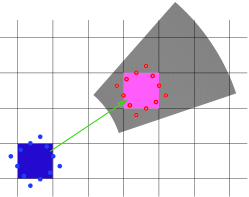
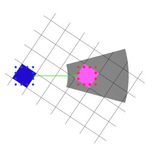
Figure 3: M2L translation from $C$ (the purple cube) to $D$ (the pink cube) in arbitrary directional cone.

The key of the matrix reduction algorithm is finding the compressing matrices $\tilde{\bm{U}}$ and $\tilde{\bm{R}}$. In SArcmp, all the M2L matrices has to be collected to generate $\tilde{\bm{U}}$ and $\tilde{\bm{R}}$. Assume the boundary is of size $D$, the size of the cubes in the highest level is $w\sim\sqrt{D/k}$, thus there are $O(D^{2}/w^{2})=O(kD)=O(\sqrt{N})$ M2L matrices in the highest level. Therefore, the computational complexity for collecting the M2L matrices and performing SVD is $O(N^{3/2})$, therefore this approach is not suitable for the fast directional algorithm. A new compressing scheme is proposed in the following section, in which the compressing matrices can be generated in the upward and downward pass, thus the matrices collecting step can be omitted to avoid this drawback.

4.1.2 Matrix reduction without matrices collecting

In the multilevel fast algorithms, evaluating the potential $\bm{p}$ in a leaf cube induced by the source densities $\bm{q}$ in another leaf cube in its far field can be computed as

$$\bm{p=TLKMSq},$$ (16)

where $\bm{S},\bm{M},\bm{K},\bm{L},\bm{T}$ are the S2M, M2M, M2L, L2L and L2T matrices, respectively. In the fast directional algorithm base on equivalent densities, the M2M matrix $M$ and L2L matrix $L$ are also computed by two steps, which are similar with S2M and L2T, as shown in Figure 2(a) and 2(c),

$$\bm{M}=\bm{G}_{\text{up}}^{+}\bm{E}_{\text{up}},$$ (17a)

$$\bm{L}=\bm{E}_{\text{dn}}\bm{G}_{\text{dn}}^{+},$$ (17b)

where $\bm{G}_{\text{up}}$ is the matrix evaluating the directional outgoing check potentials produced by the directional outgoing equivalent densities, $\bm{G}_{\text{dn}}$ is the matrix evaluating the directional outgoing incoming potentials produced by the directional incoming equivalent densities, and the superscript “+” denotes the Moore-Penrose inverse. They can be computed via performing SVD for $\bm{G}_{\text{up}}$ and $\bm{G}_{\text{dn}}$

$$\bm{G}_{\text{up}}=\bm{U}_{\text{up}}\bm{\Sigma}_{\text{up}}\bm{V}_{\text{up}}^{\text{H}},$$ (18a)

$$\bm{G}_{\text{dn}}=\bm{U}_{\text{dn}}\bm{\Sigma}_{\text{dn}}\bm{V}_{\text{dn}}^{\text{H}}.$$ (18b)

Then the Moore-Penrose inverses $\bm{G}_{\text{up}}^{+}$ and $\bm{G}_{\text{dn}}^{+}$ can be approximated by inverting (18) and truncating the columns corresponding to tiny singular values

$$\sigma_{i}<\varepsilon\sigma_{0},$$ (19)

where $\sigma_{0}$ is the largest singular value of $\bm{G}^{+}$. Thus

$$\bm{G}_{\text{up}}^{+}\approx\tilde{\bm{V}}_{\text{up}}\tilde{\bm{\Sigma}}_{\text{up}}^{-1}\tilde{\bm{U}}_{\text{up}}^{\text{H}},$$ (20a)

$$\bm{G}_{\text{dn}}^{+}\approx\tilde{\bm{V}}_{\text{dn}}\tilde{\bm{\Sigma}}_{\text{dn}}^{-1}\tilde{\bm{U}}_{\text{dn}}^{\text{H}}.$$ (20b)

Substituting (20) to (17) and (16), one gets

$$\begin{split}\bm{LKM}=&\bm{E}_{\text{dn}}\bm{G}_{\text{dn}}^{+}\bm{K}\bm{G}_{\text{up}}^{+}\bm{E}_{\text{up}}\\ \approx&\bm{E}_{\text{dn}}\tilde{\bm{V}}_{\text{dn}}\tilde{\bm{\Sigma}}_{\text{dn}}^{-1}\tilde{\bm{U}}_{\text{dn}}^{\text{H}}\bm{K}\tilde{\bm{V}}_{\text{up}}\tilde{\bm{\Sigma}}_{\text{up}}^{-1}\tilde{\bm{U}}_{\text{up}}^{\text{H}}\bm{E}_{\text{up}}.\end{split}$$ (21)

Since the directional equivalent points and the directional check points also satisfies the directional parabolic separation condition, as illustrated in Figure 2, the number of columns in truncated matrices $\tilde{\bm{U}}_{\text{dn}}$ and $\tilde{\bm{V}}_{\text{up}}$ is also $T(\varepsilon)$. Therefore, take $\tilde{\bm{U}}_{\text{dn}}$ and $\tilde{\bm{V}}_{\text{up}}$ as the compressing matrices, the M2L matrices can also be compressed into more compact form

$$\tilde{\bm{K}}=\tilde{\bm{U}}_{\text{dn}}^{\text{H}}\bm{K}\tilde{\bm{V}}_{\text{up}}.$$ (22)

4.2 Low rank decomposition for reduced M2L matrices

After the matrix reduction in Section 4.1, the resulting M2L matrices are still of low rank[24, 23], this means the M2L translations can be further accelerated by performing low rank approximations for the M2L matrices individually. In this paper, this is also done in the same way as that in [23], i.e., the low rank decomposition is achieved by SVD.

For each $k$ dimensional reduced M2L matrix $\tilde{\bm{K}}_{k\times k}$, perform SVD

$$\tilde{\bm{K}}=\bm{U}\bm{S}\bm{Q}^{\text{H}}.$$ (23)

Then truncate the columns corresponding to the tiny singular values

$$\sigma_{i}<\varepsilon\sigma_{0},$$ (24)

where $\sigma_{0}$ is the largest singular value of $\bm{K}$. Thus

$$\tilde{\bm{K}}_{k\times k}\approx\hat{\bm{U}}_{k\times r}\hat{\bm{S}}_{r\times r}\hat{\bm{Q}}_{r\times k}^{\text{H}}=\hat{\bm{U}}_{k\times r}\hat{\bm{V}}_{r\times k},$$ (25)

where $\hat{\bm{V}}_{r\times k}=\hat{\bm{S}}_{r\times r}\hat{\bm{Q}}_{r\times k}^{\text{H}}$. The translations can be more efficient when $r<\frac{1}{2}k$.

The overall accelerating approach for M2L translations are illustrated in Figure 4. Where, $\bm{K}_{m\times n}$ is the original M2L matrix, $\tilde{\bm{U}}_{m\times k}$ and $\tilde{\bm{R}}_{k\times n}$ is the compressing matrices in Section 4.1.2, $\hat{\bm{U}}_{k\times r}$ and $\hat{\bm{V}}_{r\times k}$ are the individually low rank decomposition matrices for M2L matrices.

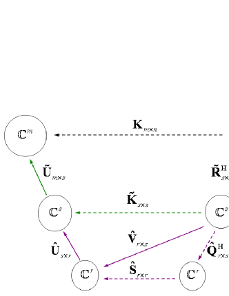
Figure 4: The accelerating approach for M2L.

4.3 Accelerating technique for upward and downward passes

It is proved in [23] that, the compressing matrices for M2L reduction can also be used to compress the translation matrices in upward and downward passes. In this paper, the compressing matrices are generated in computing the translation matrices in the upward and downward passes, and the compressing approach is simpler.

Assume $\bm{M}_{l}=\bm{G}_{\text{up},l}^{+}\bm{E}_{\text{up},l}$ is the M2M matrix translating the directional outgoing equivalent densities in the $(l+1)$-th level to the directional outgoing equivalent densities in the $l$-th level, and $\bm{S}_{l+1}=\bm{G}_{\text{up},l+1}^{+}\bm{E}_{\text{up},l+1}$ is the S2M matrix translating the sources inside a leaf cube in the $(l+1)$-th level to the directional outgoing equivalent densities in the $l$-th level. Combining with Equations (20) and (16), there is

$$\begin{split}\bm{M}_{l}\bm{S}_{l+1}=&\bm{G}_{\text{up},l}^{+}\bm{E}_{\text{up},l}\bm{G}_{\text{up},l+1}^{+}\bm{E}_{\text{up},l+1}\\ \approx&\tilde{\bm{V}}_{\text{up},l}\tilde{\bm{\Sigma}}_{\text{up},l}^{-1}\tilde{\bm{U}}_{\text{up},l}^{\text{H}}\bm{E}_{\text{up},l}\tilde{\bm{V}}_{\text{up},l+1}\tilde{\bm{\Sigma}}_{\text{up},l+1}^{-1}\tilde{\bm{U}}_{\text{up},l+1}^{\text{H}}\bm{E}_{\text{up},l+1}\\ =&\tilde{\bm{V}}_{\text{up},l}(\tilde{\bm{\Sigma}}_{\text{up},l}^{-1}\tilde{\bm{U}}_{\text{up},l}^{\text{H}}\bm{E}_{\text{up},l}\tilde{\bm{V}}_{\text{up},l+1})(\tilde{\bm{\Sigma}}_{\text{up},l+1}^{-1}\tilde{\bm{U}}_{\text{up},l+1}^{\text{H}}\bm{E}_{\text{up},l+1})\\ =&\tilde{\bm{V}}_{\text{up},l}\tilde{\bm{M}}_{\text{up},l}\tilde{\bm{S}}_{\text{up},l+1}.\end{split}$$ (26)

Where, $\tilde{\bm{V}}_{\text{up},l}$ would be used to compress the M2L matrices in $l$-th level, as shown in (22),

$$\tilde{\bm{M}}_{\text{up},l}=\tilde{\bm{\Sigma}}_{\text{up},l}^{-1}\tilde{\bm{U}}_{\text{up},l}^{\text{H}}\bm{E}_{\text{up},l}\tilde{\bm{V}}_{\text{up},l+1}$$ (27)

is the compressed M2M matrix in $l$-th level, and

$$\tilde{\bm{S}}_{\text{up},l+1}=\tilde{\bm{\Sigma}}_{\text{up},l+1}^{-1}\tilde{\bm{U}}_{\text{up},l+1}^{\text{H}}\bm{E}_{\text{up},l+1}$$ (28)

is the compressed S2M matrix in $(l+1)$-th level. The translating matrices in the downward pass compressed in the same manner, resulting

$$\tilde{\bm{L}}_{\text{dn},l}=\tilde{\bm{U}}_{\text{dn},l+1}^{\text{H}}\bm{E}_{\text{dn},l}\tilde{\bm{V}}_{\text{dn},l}\tilde{\bm{\Sigma}}_{\text{dn},l}^{-1}$$ (29)

be the compressed L2L matrix translating the directional incoming check potentials in the $l$-th level to the directional incoming check potentials in the $(l+1)$-th level, and

$$\tilde{\bm{T}}_{\text{dn},l+1}=\bm{E}_{\text{dn},l+1}\tilde{\bm{V}}_{\text{dn},l+1}\tilde{\bm{\Sigma}}_{\text{dn},l+1}^{-1}$$ (30)

be the compressed L2T matrix translating the directional incoming check potentials of a leaf cube in the $(l+1)$-th level to the target potentials.

5 Numerical studies

The performance of our fast directional algorithm for Burton-Miller formulation is demonstrated by several numerical examples. The codes are implemented serially in C++. The Burton-Miller formulation (4) is discretized by collocation method and piecewise constant elements, i.e., assume $\bm{x}_{i}$ is the centroid of the $i$-th triangular element $\triangle_{i}$, the weight functions $w_{i}(\bm{x})$ and the basis functions $\chi_{i}(\bm{x})$ are chosen to be

$$\begin{split}w_{i}(\bm{x})=&\delta(\bm{x}_{i}),\\ \chi_{i}(\bm{x})=&\delta_{ij},\quad\bm{x}\in\triangle_{j}.\end{split}$$ (31)

The resulting linear systems are solved by GMRES solver, and its converging tolerance is set to be equal to the singular value truncating threshold $\varepsilon$ in (19) and (24). All the computational results are computed on a computer with a Xeon 5450 (2.66 GHz) CPU and 32 GB RAM.

5.1 Performance of our algorithm

First let us study the performance of our algorithm, in which the equivalent points and the check points are distributed straightforwardly, and the translation operators are compressed. It is studied by a unit sphere pulsating problem. That is, the surface of the unit sphere pulsates with uniform radial velocity $v_{a}=\frac{\partial u}{\partial\bm{n}}=1$. The numerical error of the velocity potential on the surface can be computed via the analytical solution

$$u=\frac{1}{1+ik}.$$ (32)

The unit sphere is first discretized into $N=512$ triangular elements and it is used to compute the pulsating problem with $k=\pi$. That is, the diameter equals 1 wavelength. Then the mesh is refined and the wavenumber is doubled 6 times. The finest mesh has $N=2097152$ elements and the diameter of the sphere is 64 in terms of wavelength.

First let us study the influence of the number of equivalent points along each direction $p$ on the accuracy and efficiency of the algorithm. Let $p=\log(1/\varepsilon)+p_{0}$. The performance of the algorithm for different $p_{0}$ is studied by choosing $p_{0}=0,1,2,3$ for the unit sphere pulsating problem with the finest mesh and $\varepsilon=\text{1e-3}$. The results are listed in Table 1, where $T_{\text{t}}$ is the total time cost, $T_{\text{it}}$ is the running time in each iteration, $N_{\text{it}}$ is the number of iterations, and $M$ is the memory consume. It is shown that the resulting error maintains almost the same when $p_{0}\geq 1$, while the total time cost is considerably increased. Therefore, we choose $p_{0}=1$ for the following examples.

Table 1: Results of the unit sphere pulsating problem with different number of equivalent points $N=2097152,\varepsilon=\text{1e-3}$.

$p_{0}$	$T_{\text{t}}(s)$	$T_{\text{it}}$(s)	$N_{\text{it}}$	$M$(MB)	$L_{2}$-error
0	12067.8	274.75	8	24451.2	1.90e-2
1	14250.9	260.45	4	27822.7	3.90e-3
2	18268.9	260.20	4	27846.2	3.37e-3
3	23543.5	325.01	4	27526.2	3.24e-3

The results for the unit sphere pulsating problem are listed in Table 2. The case with $N=2097152,\varepsilon=\text{1e-4}$ is not computed because of memory constraint. It is shown that the complexity of our algorithm grows almost linearly with respect to the number of degrees. The resulting error concludes the discretization error of BEM and the approximating error $\varepsilon$ of the fast algorithm. The resulting error for meshes with less than $32768$ elements preserves almost the same with $\varepsilon=\text{1e-3}$ and 1e-4, which shows that the resulting error is bounded by the precision of the boundary integral discretization. The errors for finer meshes maintain almost the same with $\varepsilon=\text{1e-3}$, this is because they are bounded by the accuracy of the fast accelerating scheme. The error continue decreasing at the same rate with $\varepsilon=\text{1e-4}$, which indicates that the error of the fast accelerating scheme is smaller and more precise results can be obtained by decreasing $\varepsilon$. That is, the error can be reduced linearly to $O(\varepsilon)$, which indicates that our fast algorithm is quite stable.

Table 2: Results of the unit sphere pulsating problem

$N$	$k$	$T_{\text{t}}$(s)	$T_{\text{it}}$(s)	$N_{\text{it}}$	$M$(MB)	$L_{2}$-error
$\varepsilon=$1e-3
512	$\pi$	1.76	0.02	3	4.59	3.65e-2
2048	$2\pi$	4.26	0.07	3	19.99	1.86e-2
8192	$4\pi$	50.95	0.46	3	119.76	9.26e-3
32768	$8\pi$	166.85	2.63	3	346.67	4.84e-3
131072	$16\pi$	962.98	13.79	3	2088.75	3.11e-3
524288	$32\pi$	3427.14	69.15	3	6761.24	2.92e-3
2097152	$64\pi$	14250.90	260.45	4	27822.70	3.90e-3
$\varepsilon=$1e-4
512	$\pi$	2.63	0.02	6	8.98	3.65e-2
2048	$2\pi$	8.53	0.16	5	39.66	1.85e-2
8192	$4\pi$	54.89	0.74	4	192.34	9.27e-3
32768	$8\pi$	254.08	5.66	4	499.10	4.63e-3
131072	$16\pi$	1490.30	29.58	5	2920.10	2.35e-3
524288	$32\pi$	5457.84	143.36	6	9223.96	1.32e-3

5.2 Comparison to the wideband FMM

To compare the performance of the current fast directional algorithm with the wideband fast multipole method, the unit sphere scattering problem in Section 4.1 in [25] is computed. The point source is at (-2, 0, 0). Two cases with $k=5.0$ and $k=50$ are computed. The sphere surface is discretized into approximately the same number of elements with that in [25], and we chose $\varepsilon=1e-3$. The results are listed in Table 3. Note that the wideband FMM is parallelized and performed by a four core computer with a 64-bit Intel Core${}^{\text{TM}}$ 2 Duo CPU, thus it should be about 4 times faster. However, it is shown that, our algorithm consumes almost the same time when $ka=50.0$ and is much faster when $ka=5.0$. Therefore, our algorithm is much more efficient than the wideband fast multipole algorithm.

Table 3: Comparison of results for sphere scattering problems reported in Ref. [25] and the present study.

	$k$	$N$	cores	$T_{\text{it}}$(s)
[25]	5.0	101270	4	7.08
Present	5.0	106032	1	2.15
[25]	50.0	101270	4	10.84
Present	50.0	106032	1	12.38

5.3 Plane wave scattering problems

For plane wave scattering problems, two sound-hard obstacles are considered, and the incident plane wave is assumed to be propagating in (1, 0, 0) direction. The singular truncating threshold and the GMRES converging tolerance is set to be $\varepsilon=\text{1e-3}$. The triangular meshes used in the examples have a refinement of approximately 16 elements per wavelength.

First the sound-hard unit sphere scattering problem is calculated. The sphere diameter is 64 wavelengths, i.e., $k=201$. The sphere surface is discretized into 2097152 triangular elements. The total time cost for solving the problem $T_{\text{t}}=$ 8690s, the time cost in each iteration $T_{\text{it}}=$ 260.3s, the number of iterations $N_{\text{it}}=14$, the memory consumption $M=$ 26.2GB. The resulting acoustic velocity potential on the surface is illustrated in Fig. 5(a), and the scattering field on the surface is illustrated in Fig. 5(b). It is shown that our numerical results agrees quite well with the analytical solution.

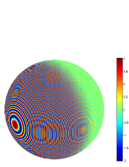
(a) Acoustic field.

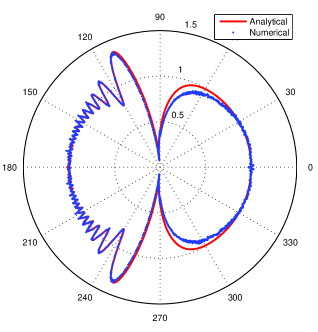
(b) Scattering velocity potential.

Figure 5: Resulting of the unit sphere scattering problem.

The second model is a Su-27 fighter which is 21.49 meters long. We set $k=30$, thus its size is 102.7 wavelengths. The surfaces are discretized into 4143908 triangular elements. The total time cost for solving the problem $T_{\text{t}}=$ 38799.3s, the time cost in each iteration $T_{\text{it}}=$ 133.57s, the number of iterations $N_{\text{it}}=256$ without any preconditioner. The memory consumption $M=$ 25.08GB. The resulting acoustic velocity potential on the surface is illustrated in Fig. 6.

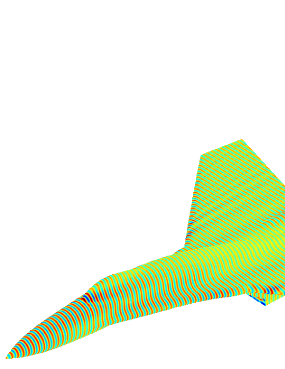
Figure 6: Resulting of the Su-27 scattering problem.

The second model is a submarine which is 80 meters long. We set $k=12.5$, thus $kD=1000$ and its size is 159 wavelengths. The surfaces are discretized into 4041088 triangular elements. The total time cost for solving the problem $T_{\text{t}}=$ 13648s $\approx$ 3.8h, the time cost in each iteration $T_{\text{it}}=$ 204.14s, the number of iterations $N_{\text{it}}=35$ without any preconditioner. The memory consumption $M=$ 24.73GB. The resulting acoustic velocity potential on the surface is illustrated in Fig. 7.

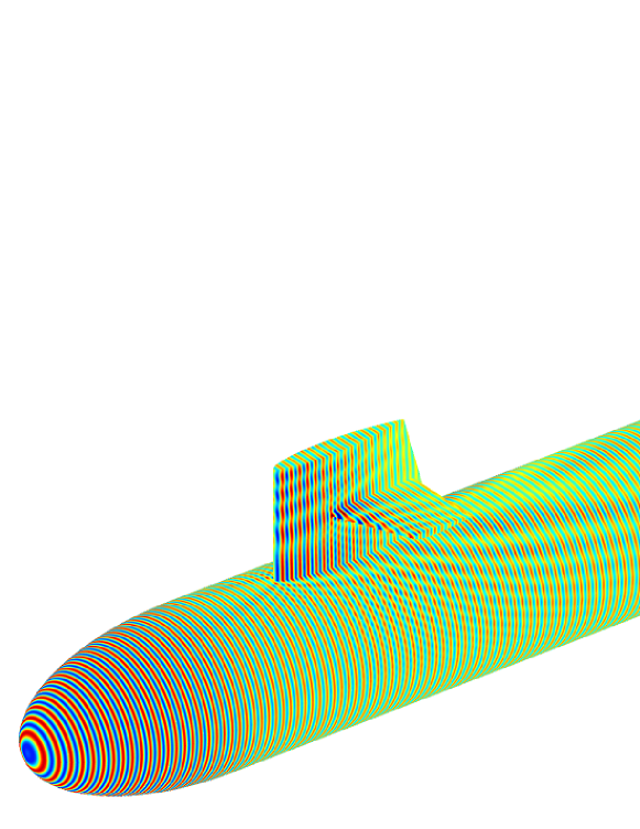
Figure 7: Resulting of a submarine scattering problem.

6 Conclusion

In this paper, the fast directional algorithm is adapted to accelerate the acoustic problem computations with Burton-Miller formulation. Although there are four integrals in the Burton-Miller formulation, they can be evaluated efficiently by two fast summing approach. The outgoing equivalent points and the outgoing check points are sampled directly instead of by pseudo skeleton approach, resulting in a simpler fast directional algorithm. Then all the translations are accelerated by matrix reduction and low-rank approximation, which is similar with the SArcmp approach, while the compressing matrices are generated in advance, and no matrix collection is required. The accuracy and efficiency of the algorithm are examined by numerical results. It is shown that the acoustic scattering problems with over 4 million DOFs and $kD=1000$ can be computed in less than 4 hours.

References

- [1] L. Greengard and V. Rokhlin. A fast algorithm for particle simulation. Journal of Computational Physics, 73:325–348, 1987.
- [2] L. Greengard and V. Rokhlin. A new version of the fast multipole method for the Laplace equation in three dimensions. Acta Numerica, 6(1):229–269, 1997.
- [3] Eric Darve. The fast multipole method: Numerical implementation. Journal of Computational Physics, 160:195–240, 2000.
- [4] W. Hackbusch. A sparse matrix arithmetic based on H-matrices. Part I: Introduction to H-matrices. Computing, 62:89–108, 1999.
- [5] W. Hackbusch and Z. P. Nowak. On the fast matrix multiplication in the boundary element method by panel clustering. Numerische Mathematik, 54:463–491, 1989.
- [6] Mario Bebendorf. Approximation of boundary element matrices. Numerische Mathematik, 86:565–589, 2000.
- [7] Mario Bebendorf and Sergej Rjasanow. Adaptive low-rank approximation of collocation matrices. Computing, 70:1–24, 2003.
- [8] G. Beylkin, R. Coifman, and V. Rokhlin. Fast wavelet transforms and numerical algorithms. Pure Appl. Math., 37:141–183, 1991.
- [9] Johannes Tausch. A variable order wavelet method for the sparse representation of layer potentials in the non-standard form. Journal of Numerical Mathematics, 12(3):233–254, 2004.
- [10] Joel R. Phillips and Jocob K. White. A precorrected-FFT method for electrostatic analysis of complicated 3-D structures. IEEE Transactions on Computer-Aided Design of Integrated Circuits and Systems, 16(10):1059–1072, 1997.
- [11] Zai You Yan and Xiao Wei Gao. The development of the pFFT accelerated BEM for 3-D acoustic scattering problems based on the Burton and Miller’s integral formulation. Engineering Analysis with Boundary Elements, 37:409–418, 2013.
- [12] Oscar P. Bruno and Leonid A. Kunyansky. A fast, high-order algorithm for the solution of surface scattering problems: Basic implementation, tests, and applications. Journal of Computational Physics, 110:80–110, 2001.
- [13] Oscar P. Bruno, Tim Elling, and Catalin Turc. Regularized integral equations and fast high-order solvers for sound-hard acoustic scattering problems. International Journal of Numerical Methods in Engineering, 91:1045–1072, 2012.
- [14] V. Rokhlin. Diagonal forms of translation operators for the Helmholtz equation in three dimensions. Applied and Computational Harmonic Analysis, 1:82–93, 1993.
- [15] Hongwei Cheng, William Y. Crutchfield, Zydrunas Gimbutas, Leslie F. Greengard, J. Frank Ethridge, Jingfang Huang, Vladimir Rokhlin, Norman Yarvin, and Junsheng Zhao. A wideband fast multipole method for the Helmholtz equation in three dimensions. Journal of Computational Physics, 216:300–325, 2006.
- [16] Nail A. Gumerov and Ramani Duraiswami. A broadband fast multipole accelerated boundary element method for the three dimensional Helmholtz equation. Journal of the Acoustical Society of America, 125(1):191–205, 2009.
- [17] Björn Engquist and Lexing Ying. Fast directional multilevel algorithms for oscillatory kernels. SIAM J. Sci. Comput., 29(4):1710–1737, 2007.
- [18] Björn Engquist and Lexing Ying. Fast directional algorithms for the Helmholtz kernel. Journal of Computational and Applied Mathematics, 234:1851–1859, 2010.
- [19] Matthias Messner, Martin Schanz, and Eric Darve. Fast directional multilevel summation for oscillatory kernels based on Chebyshev interpolation. Journal of Computational Physics, 231(4):1175–1196, 2012.
- [20] Mario Bebendorf, Christian Kuske, and Raoul Venn. Wideband nested cross approximation for Helmholtz problems. Number 536, Bonn, December 2012.
- [21] R. Kress. Minimizing the condition number of boundary integral operators in acoustic and electromagnetic scattering. Quarterly Journal of Mechanics & Applied Mathematics, 38(2):323–341, 1985.
- [22] Lexing Ying, George Biros, and Denis Zorin. A kernel-independent adaptive fast multipole algorithm in two and three dimensions. Journal of Computational Physics, 196:591–626, 2004.
- [23] Yanchuang Cao, Lihua Wen, and Junjie Rong. A SVD accelerated kernel-independent fast multipole method and its application to BEM. arXiv: 1211.2517v2, pages 1–19, 2012.
- [24] Matthias Messner, Berenger Bramas, Olivier Coulaud, and Eric Darve. Optimized M2L kernels for the Chebyshev interpolation based fast multipole method. arXiv preprint, arXiv:1210.7292, pages 1–23, 2012.
- [25] W. R. Wolf and S. K. Lele. Wideband fast multipole boundary element method: Application to acoustic scattering from aerodynamic bodies. International journal for numerical methods in fluids, 67:2108–2129, 2011.