Stronger findings from mass spectral data through multi-peak modeling

Abstract

Mass spectrometry-based metabolomic analysis depends upon the identification of spectral peaks by their mass and retention time. Statistical analysis that follows the identification currently relies on one main peak of each compound. However, a compound present in the sample typically produces several spectral peaks due to its isotopic properties and the ionization process of the mass spectrometer device. In this work, we investigate the extent to which these additional peaks can be used to increase the statistical strength of differential analysis.

We present a Bayesian approach for integrating data of multiple detected peaks that come from one compound. We demonstrate the approach through a simulated experiment and validate it on ultra performance liquid chromatography-mass spectrometry (UPLC-MS) experiments for metabolomics and lipidomics. Peaks that are likely to be associated with one compound can be clustered by the similarity of their chromatographic shape. Changes of concentration between sample groups can be inferred more accurately when multiple peaks are available.

When the sample-size is limited, the proposed multi-peakapproach improves the accuracy at inferring covariate effects. An R implementation, data and the supplementary material are available at http://research.ics.aalto.fi/mi/software/peakANOVA/.

1 Introduction

The study of changes in the levels of metabolites and lipids has become essential for the comprehensive understanding of human health [18]. Mass spectrometry (MS) techniques have become the standard method for characterizing the human metabolome [17] and lipidome [14]. The technique generates a spectrum of peaks in the plane defined by the retention time and the mass-to-charge ratio of an observed particle. Each peak in this plane is either generated by a particle arising from one of the compounds present in the sample, or is an artifact of the measurement without association to any of the compounds. The association between the peaks and compounds is unknown a priori. The produced peak data are noisy: First, sample preparation introduces sources of uncertainty that propagate to the analysis [5]. Second, the accuracy of the device is limited [22] and it produces biases. Third, peak identification, annotation and pre-processing steps produce additional layers of uncertainty [19]. The effect of errors at all these levels is exacerbated by the “small $n$, large $p$” problem: experiments cover a very limited number of samples, $n$, while the set of compounds measured, $p$, is potentially large.

However, there also is strong informative structure in the data: First, each compound may generate multiple adduct peaks [10] (Figure 1) and isotope peaks [12, 3] (Figure 2), whose positions and shapes provide information about the identity of the compound. Second, the concentrations of different compounds generated by or participating in similar biological processes may be highly correlated [20]. An increasing number of machine learning algorithms are being developed for inferring such structure either from raw spectral data [8] or from processed intensity data [2]. The inference of covariate effects—the differences between sample groups determined by external covariates such as an intervention—is in the core of the comparative analysis of spectral profiles [11]. In this work, we propose an unsupervised approach for inferring covariate effects from the data more accurately through the modeling of multiple peaks arising from a single compound (Figure 3).

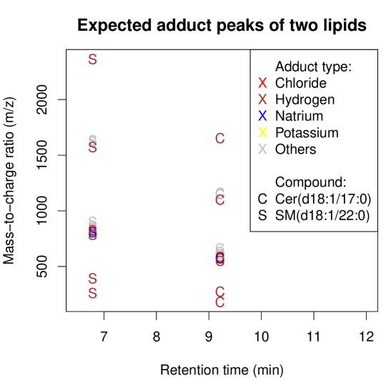
Figure 1: A schematic of the positions of typical adduct peaks [10] in the RT-m/z plane for two lipids, the ceramide Cer(d18:1/17:0) and the sphingomyelin SM(d18:1/22:0). An adduct peak is formed by an ion attaching to the compound. At the finer detail, each peak in the figure consists of multiple isotope peaks few atomic units apart, as shown for Cer(d18:1/17:0) in Figure 2. Even though the distinct isotope peaks are not visible to the eye here, they are clearly separable by the mass spectrometer. In the figure, adduct types and compounds are marked by colors and characters, respectively.

Figure 2: Natural isotopic distribution of the mass of a typical lipid, the ceramide Cer(d18:1/17:0). The presence of atomic isotopes leads to the appearance of multiple mass spectral peaks from the compound. The isotope peaks have distinct mass-to-charge ratios at the same retention time (Figure 1).

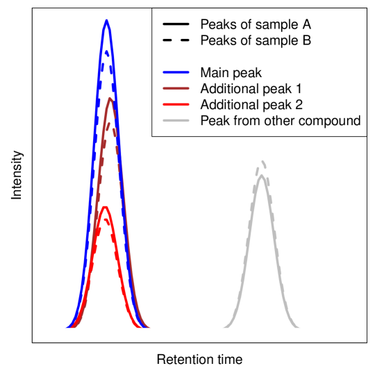
Figure 3: Schematic of spectral peaks in two samples. Peaks on the left arise from one compound while peaks on the right arise from another compound. The heights of the peaks from one compound have a constant relative difference between the two samples (solid and dashed lines), which can be used to improve the accuracy of analysis. Distinct peaks from one compound (marked by colors) have distinct mass-to-charge ratios but they share the same retention time.

The existence of additional peaks in the spectrum is usually seen as a problem and only the main peak of each identified compound is used for further analysis. All peaks are a result of the ionisation process where a charged particle is attached to or detached from a compound. Each compound-ion pair produces a distinct adduct or deduct peak. Random variation in the ionisation process leads to inconsistencies between batches of samples, perceived as variation in the ratio of intensities of the peaks associated with one compound. This is a major source of error for all existing analysis approaches regardless of the choice of the peak used for the analysis. On the other hand, the distribution of the intensities of isotope peaks is by nature well preserved across both samples and compounds. Moreover, the natural isotopic distribution of a compound is known and can be used to make peak annotation more precise. In this way, isotope peaks provide reliable additional information about the differences in compound concentrations between sample groups.

We propose a probabilistic approach for extending statistical analysis to all available peaks and show that the additional peaks can provide a real benefit to the inference of covariate effects in an experiment. The approach is used to cluster the peaks that are likely to arise from a single compound together and to infer the changes in concentrations of the compounds more accurately based on all these peaks. By this approach, we are addressing the problem of inadequate sample-size by introducing additional data describing the compounds behind the noisy measurements.

To solve the problem we introduce the following assumptions about the generative process of the data within a Bayesian model: First, samples carry between-group differences in their compound concentrations and the differences arise from responses to external covariates. Second, multiple observed spectral peaks follow an identical generative process and their heights are a noisy reflection of the true concentration level of the compound. Third, shapes of the peaks from one compound are generated through an identical process following the properties of the measurement device, and thus these shapes are highly similar.

The approach presented in this paper consists of two stages of computational inference: (1) peaks that share a compound as their generative source are clustered together, and (2) the responses to external covariates are inferred on these groups of peaks.

The clustering part of the approach is based on a nonparametric Bayesian Dirichlet process model [16]. To improve the performance of the clustering model, we have redefined the prior distributions of the model to have a better match to the distribution of the peak shape similarity observations than in the original proposition.

The model for inferring the responses to covariates operates on clusters inferred in the first part. A Bayesian multi-way model [11] is suitable for this task. This model itself could be used for clustering summarized mass spectral intensity data, but in this work, we demonstrate that the clustering can be done more accurately based upon the similarity of chromatographic peak shapes.

2 Methods

This section describing the models consists of two parts: clustering of spectral peaks and inference of covariate effects. To maintain the mathematical rigor in the section, we use the terms “samples,” “variables” and “clusters,” to refer to the experimental runs of the mass spectrometer, the peaks in the mass spectrometry data, and the yet unknown compounds in the experimental runs, respectively. In the equations, we denote samples, variables and clusters by the indices $i$, $j$ and $k$, respectively:

$$\begin{split}i=&1,\ldots,N\hskip 5.0pt\text{(samples, {i.e.}, experimental runs)},\\ j=&1,\ldots,P\hskip 5.0pt\text{(variables, {i.e.}, peaks)},\\ k=&1,\ldots,K\hskip 5.0pt\text{(clusters, {i.e.}, compounds)},\end{split}$$ (1)

where $N$, $P$ and $K$ are their total numbers.

2.1 Clusters of peaks based on the similarity

Following earlier work [16], we measure the similarity between the shapes of two peaks by their correlation computed over a window of retention time after a standard peak alignment [15] across the samples. Truncating negative values to zero, this leads to a distinct similarity matrix $\mathbf{Q}_{i\cdotp\cdotp}~{}\in~{}[0,1]^{P\times P}$ for each sample $i$. In the notation, the operator “$\cdot$” indicates that the entire dimension of the array is included, not only the single item $j$. Because a peak is not necessarily observed in every sample, there may be missing values in the matrices. Therefore, we construct an additional mask $\mathbf{R}~{}\in~{}\{0,1\}^{N\times P\times P}$ with binary values $r_{ijj^{\prime}}$ indicating whether peaks $j$ and $j^{\prime}$ have any overlap in sample $i$.

2.1.1 Model

We assume that the peaks are generated through a Dirichlet process [6]: there is an unknown number of clusters and an unknown and variable number of peaks that arise from each of the clusters. Peaks are assumed to have a one-out-of-many association: each peak is associated with only one of the unknown clusters. With these basic assumptions, we can infer the $P$-by-$K$ clustering matrix $\mathbf{V}$ from the data $\mathbf{Q}$. To make the following equations more compact, we use an additional variable $\varepsilon_{jj^{\prime}}~{}=~{}\mathbf{v}_{j\cdotp}\mathbf{v}_{j^{\prime}\cdotp}^{\text{T}}~{}\in~{}\{0,1\}$, which is an inner product of the cluster indicator vectors of the peaks $j$ and $j^{\prime}$, to denote whether the two peaks come from the same or different clusters (1 or 0, respectively).

We set a spike-and-slab prior [13] for the peak shape similarity to model the inherent sparse structure of the data. The similarity between any pair of observed peaks ($j,j^{\prime}$) is assumed to follow a beta distribution, but the shape of the distribution is assumed to depend on whether the pair comes from the same cluster or from different clusters (shape parameters $\left(a_{\text{in}},b_{\text{in}}\right)$ or $\left(a_{\text{out}},b_{\text{out}}\right)$, when $\varepsilon_{jj^{\prime}}=1$ or $0$, respectively). Also the probability of a missing similarity value is assumed to depend on the cluster assignment of the pair ($p_{0}^{\text{in}}$ or $p_{0}^{\text{out}}$, when $\varepsilon_{jj^{\prime}}=1$ or $0$, respectively). The distributional assumptions are summarized as

$$p\left(q_{ijj^{\prime}},r_{ijj^{\prime}}=1|\varepsilon_{jj^{\prime}}=1\right) =\left(1-p_{0}^{\text{in}}\right)\text{Beta}\left(q_{ijj^{\prime}}|a_{\text{in}},b_{\text{in}}\right)$$ (2)

$$p\left(q_{ijj^{\prime}},r_{ijj^{\prime}}=0|\varepsilon_{jj^{\prime}}=1\right) =p_{0}^{\text{in}}\delta\left(r_{ijj^{\prime}}\right)$$ (3)

for a pair of peaks in the same cluster and

$$p\left(q_{ijj^{\prime}},r_{ijj^{\prime}}=1|\varepsilon_{jj^{\prime}}=0\right) =\left(1-p_{0}^{\text{out}}\right)\text{Beta}\left(q_{ijj^{\prime}}|a_{\text{out}},b_{\text{out}}\right)$$ (4)

$$p\left(q_{ijj^{\prime}},r_{ijj^{\prime}}=0|\varepsilon_{jj^{\prime}}=0\right) =p_{0}^{\text{out}}\delta\left(r_{ijj^{\prime}}\right)$$ (5)

for a pair of peaks in different clusters. The Dirac delta function $\delta$, which is a point mass at zero, constitutes the “spike” of the two-component mixture distribution.

Combining Equations from 2 to 5, the likelihood of the entire peak shape data becomes a product over all peak pairs and samples:

$$\begin{split}\mathcal{L}\left(\mathbf{Q},\mathbf{R}|\mathbf{V}\right)=\prod_{i=1}^{N}\prod_{j=1}^{P-1}\prod_{j^{\prime}=j+1}^{P}&p\left(q_{ijj^{\prime}},r_{ijj^{\prime}}|\varepsilon_{jj^{\prime}}=1\right)^{\varepsilon_{jj^{\prime}}}\\ &\times p\left(q_{ijj^{\prime}},r_{ijj^{\prime}}|\varepsilon_{ijj^{\prime}}=0\right)^{1-\varepsilon_{jj^{\prime}}}.\end{split}$$ (6)

We introduce a Dirichlet process prior for assigning peaks into clusters. In the non-parametric model, the probability of assigning peak $j$ to an existing cluster $k$,

$$p\left(v_{jk}=1|\mathbf{Q},\mathbf{R},\mathbf{V}_{\cdotp,-k}\right)\propto s_{k}\mathcal{L}\left(\mathbf{Q},\mathbf{R}|\mathbf{V}_{-j,\cdotp},v_{jk}=1\right),$$ (7)

is proportional to the likelihood of the peak given the cluster, weighted by the current size of the cluster, $s_{k}=\mathbf{v}_{-j,k}^{\text{T}}\mathbf{v}_{-j,k}$. In the notation, matrices $\mathbf{V}_{\cdotp,-k}$ and $\mathbf{V}_{-j,\cdotp}$ correspond to the matrix $\mathbf{V}$ with the row $k$ and the column $j$ omitted, respectively. Alternatively, with probability

$$p\left(v_{j,K+1}=1|\mathbf{Q},\mathbf{R},\mathbf{V}\right)\propto\alpha_{\text{DP}}\mathcal{L}\left(\mathbf{Q},\mathbf{R}|\mathbf{V}_{-j,\cdotp},v_{j,K+1}=1\right),$$ (8)

the process may create a new cluster with the index $K+1$ and only the peak $j$ inside. Now the likelihood term is weighted by the Dirichlet process concentration parameter $\alpha_{\text{DP}}$.

2.1.2 Inference

We infer the posterior distribution of the clustering via Gibbs sampling, which results in a set of $S$ samples of the clustering $\mathbf{V}^{(s)}$, $s=1,\ldots,S$, from the true posterior distribution $p\left(\mathbf{V}|\mathbf{Q},\mathbf{R}\right)$. Further analysis can operate on the entire posterior distribution of the clustering through integration or on a point estimate of the distribution.

We follow earlier work [4] and acquire a point estimate of the posterior distribution of the clustering through finding the least-squares clustering: the posterior sample $s$ whose adjacency matrix $\mathbf{V}^{(s)}\mathbf{V}^{(s)\text{T}}$ has the smallest squared deviation from the posterior pairwise probabilities $\boldsymbol{\Pi}$ of the peaks. The index of the least-squares clustering thus is

$$s_{\text{LS}}=\operatorname*{arg\,min}_{s\in\{1,\ldots,S\}}\sum_{j=1}^{P-1}\sum_{j^{\prime}=j+1}^{P}\left(\mathbf{v}_{j\cdot}^{(s)}\mathbf{v}_{j^{\prime}\cdot}^{(s)\text{T}}-\widehat{\pi}_{jj^{\prime}}\right)^{2},$$ (9)

where the posterior pairwise probabilities

$$\widehat{\boldsymbol{\Pi}}=\frac{1}{S}\sum_{s=1}^{S}\mathbf{V}^{(s)}\mathbf{V}^{(s)\text{T}}$$ (10)

are estimated as the average adjacency matrix over the posterior samples.

2.2 Covariate effects based on peak heights

Having inferred the grouping of similar peaks into clusters that each correspond to a compound, we infer the differences in concentrations between sample groups for each cluster given the peak height data $\mathbf{X}~{}\in~{}\mathbb{R}^{P\times N}$ and the clustering $\mathbf{V}$. Again, there may be missing values in the data.

2.2.1 Model

After a peak-specific centering based on the control group, the observed peak heights for each sample $i$ are assumed to be normally distributed with a cluster-specific mean $\mathbf{x}_{\cdotp i}^{\text{lat}}$:

$$\mathbf{x}_{\cdotp i}|\mathbf{V},\mathbf{x}^{\text{lat}},\boldsymbol{\sigma}^{2}\sim\mathcal{N}\left(\mathbf{V}\mathbf{x}^{\text{lat}}_{\cdotp i},\boldsymbol{\Lambda}\right),$$ (11)

where the diagonal matrix $\boldsymbol{\Lambda}$ contains the peak-specific variance parameters $\boldsymbol{\sigma}^{2}~{}\in~{}\mathbb{R}_{+}^{P}$. The cluster-specific means are assumed to be normally distributed with a sample group-specific prior $\boldsymbol{\alpha}$,

$$\mathbf{x}^{\text{lat}}_{\cdotp i}|\boldsymbol{\alpha},a_{i}\sim\mathcal{N}\left(\boldsymbol{\alpha}_{\cdotp a_{i}},\mathbf{I}\right),$$ (12)

where $a_{i}\in\{1,\ldots,L_{a}\}$ is an indicator of group membership (covariate level) for sample $i$ and $\mathbf{I}$ is a $K\text{-by-}K$ identity matrix. The corresponding covariate effects are arranged into an $K$-by-$L_{a}$ matrix $\boldsymbol{\alpha}$ and the effects are assumed to be independent and normally distributed,

$$\boldsymbol{\alpha}_{\cdotp l}\sim\left\{\begin{array}[]{rl}\delta\left(\boldsymbol{\alpha}_{\cdotp l}\right),&l=1\\ \mathcal{N}\left(\mathbf{0},\mathbf{I}\right),&l=2,\ldots,L_{a},\end{array}\right.$$ (13)

except for the first level, $l=1$, which is defined as the baseline level and thus is fixed to zero.

The model is not limited to one covariate. For an arbitrary number of covariates, the cluster-specific means (Equation 12) can be expressed as a sum of individual covariate effects and the interaction effects of two or more covariates. This generalization can be written as

$$\mathbf{x}^{\text{lat}}_{\cdotp i}|\mathbf{E},\mathbf{C}\sim\mathcal{N}\left(\mathbf{Ec}_{\cdotp i},\mathbf{I}\right),$$ (14)

where $\mathbf{C}$ is an $L$-by-$N$ binary matrix, whose column $i$ indicates the known levels of all the covariates and all their resulting interaction levels for sample $i$. The matrix $\mathbf{E}$ has dimensions $K$-by-$L$ and its row $k$ contains the effects $\mathbf{e}_{k\cdotp}$ of the respective covariates and their interactions for cluster $k$. Similarly, Equation 13 can then be generalized as

$$\mathbf{e}_{\cdotp l}\sim\delta\left(\mathbf{e}_{\cdotp l}\right),$$ (15)

when any of the covariates is at the base level, and

$$\mathbf{e}_{\cdotp l}\sim\mathcal{N}\left(\mathbf{0},\mathbf{I}\right)$$ (16)

otherwise.

The peak-specific variance parameter

$$\sigma_{j}^{2}\sim\text{Scale-Inv-}\mathcal{\chi}^{2}\left(n_{0},\sigma_{0}^{2}\right)$$ (17)

follows a scaled inverse-$\chi^{2}$ distribution with $n_{0}$ prior samples and a scale $\sigma_{0}^{2}$.

2.2.2 Inference and analysis

We infer the covariate effects via Gibbs sampling. Now the clustering matrix $\mathbf{V}$ has been learned earlier, and is thus taken as known in the model. The posterior distributions of the covariate effects $\boldsymbol{\alpha}$ are descriptive of the differences between the sample groups and thus interesting from the analysis point of view. To assess the significance of the difference between a sample group $c>1$ and the control group $c=1$ for a cluster $k$, we can study the posterior probability of the effect $\boldsymbol{\alpha}_{kc}$ being greater or smaller than zero.

3 Results

We demonstrate the performance of the proposed method through three experiments: a simulated data experiment, a spike-in benchmark experiment with known changes in concentrations, and a gene silencing experiment with measurements of the lipidome of cancer cells.

Evaluation of the performance on real data sets is not a trivial task, as there is no ground truth available: neither the identity of the peaks nor the true effect sizes are known. Thus, we also use spike-in data, where the true covariate effects are known, although only a small number of the peaks are annotated.

For the simulated and benchmark experiments, we can compute the mean squared error (MSE) between inferred and true covariate effects and use that as an evaluation metric. As a result of the $\log$-transformation of the intensity data, we are quantifying relative changes between sample groups, independent of the average height of each peak. In the model, we thus assume that the change is preserved across the peaks of one compound, in relative terms. The significance of the difference in the MSE of the proposed approach and the comparison method is tested by a paired one-sided $t$-test. The false discovery rate is controlled by the Benjamini-Hochberg step-up procedure [1] at level 0.01. Additionally for the simulated experiment, we can study the inference of the statistical significance of effects, as the true distribution of the data is known.

To assess the sensitivity of the approaches to noise in natural lipidomic data lacking a ground truth, we use two types of indirect evaluation: First, we study the consistency of the inferred covariate effects given a prior assumption about their similarity. Second, we examine the robustness of the inferred covariate effects to noise. Finally, we demonstrate differences between the multi-peak and single-peak approaches through examples of qualitative analysis of annotated peak clusters.

We compare the performance of the following approaches and refer to them as Models 1, 2 and 3:

1. the multi-peak approach using both peak shape and height information, as proposed in this work (nonparametric clustering of peaks by their shape similarity, inference of covariate effects on the clusters based on the height of the peaks),

2. the multi-peak approach using peak height information only [11] (clustering of peaks and inference of covariate effects based on the height of the peaks only),

3. the typical single-peak approach (inference of covariate effects by the height of the strongest annotated peak only).

For the studied real data sets, we discover that peak height information alone is not enough for clustering the peaks into individual compounds due to the high level of noise and strong correlations between compounds. Thus, for real data we compare Model 1 to Model 3 and highlight the benefit gained by using peak shape information.

3.1 Simulated data

3.1.1 Introduction

We start by investigating the performance of the proposed approach on synthetic data, where the true covariate effects are known. We focus on a usual task in exploratory analysis of biological data: the detection of significant non-zero covariate effects. We measure the performance by the accuracy at this task—the ratio of true positive and true negative significant differences among all effects. We use the 95 % posterior quantiles to determine the significance. Additionally, we compute the MSE to the true effects and follow earlier work [21] at studying the performance of the two clustering models by computing the normalized information distance (NID) to the true clustering.

The approaches are tested across a set of potential experimental settings to study how the observation of additional peaks and samples affect the performance. Simulated data are generated by assuming the latent structure of Model 1. The following data parameters are varied on a grid: sample-size $N=2\times\{3,7,15\}$ and peak-specific noise $\sigma^{2}=\{1,5\}$. Additionally, the number of peaks per cluster are varied between 3, 7 and 15. Covariate effects $\boldsymbol{\alpha}_{\cdotp 2}=[2,-1,0.5,0,0,0,0]$ are generated for each data set. The experiment is repeated 100 times with independent data sets.

3.1.2 Result

On normal level of noise ($\sigma^{2}=1$), the multi-peak approaches (Models 1 and 2) always perform better at detecting significant covariate effects than the single-peak approach (Model 3; Figure 4a) and only with enough samples the performance of Model 2 becomes comparable to Model 1. The inferred clustering of Model 1 is perfect while the clustering performance of Model 2 is heavily dependent on the number of samples available (Figure 4c).

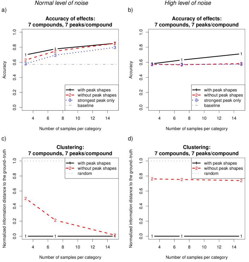
Figure 4: The use of data from multiple peaks and the peak shape information increase the accuracy at detecting significant covariate effects on simulated data. Accuracy of Models 1, 2 and 3 for simulated data is shown as a function of the sample-size in two settings: normal and high level of noise (left: $\sigma^{2}=1$, and right: $\sigma^{2}=5$, respectively). Top (a-b): Accuracy at inferring the significance of the generated covariate effects. Bottom (c-d): Normalized information distance (NID) between the inferred and the true clustering. An entirely random and an exactly correct clustering correspond to a NID of 1 and 0, respectively.

On high level of noise ($\sigma^{2}=5$), only Model 1 works (Figure 4b). The reason for the failure of Model 2 is the imperfectly inferred clustering (Figure 4d). The good performance of Model 1 comes from the clustering step, which is robust to noise in the peak heights. The peak shape similarity yields strong evidence for inferring the clusters already from a single sample.

The MSE between the inferred and true covariate effects for Model 1 is smaller compared to Model 3 in all 24 setups of the experimental grid. The difference is statistically significant in 22 setups and in all setups at the high level of noise.

The performance of the multi-peak approaches clearly improves, when more peaks from a cluster are present in the data (Figure 5). This is pronounced at a high level of noise, when the observation of a single peak is unreliable for inferring the covariate effects. In a similar way as in averaging over samples, the model is able to overcome peak-specific noise also by averaging over multiple peaks.

Figure 5: The performance of Model 1 improves when more peaks per compound are available in the simulated data. Curves A, B and C show the accuracy as a function of sample-size for simulated data with 15, 7 and 3 peaks per compound, respectively.

3.2 Benchmark data with known changes
in concentrations

3.2.1 Introduction

In the first demonstration on real UPLC-MS data [7], we show that Model 1 can infer the artificial perturbations in a spike-in experiment more accurately than the single-peak approach. The recently-published benchmark data set of apple samples includes a set of annotated spike-in compounds with increases of 20, 40 or 100 % in concentrations.

We start with the raw spectral data  in order to acquire the shapes of the peaks in addition to their heights. The mass spectra are pre-processed using MZmine 2 [15] (Section 3 in Supplementary material).

We evaluate the approaches by the MSE between inferred and true covariate effects. If the cluster contains multiple annotated peaks, the effect of each annotated peak is evaluated separately for the single-peak approach. Clusters with no annotated peaks are considered to have a 0 % true effect and the effect of the single-peak approach is inferred based on the strongest peak of the cluster.

3.2.2 Result

All clusters with annotated peaks are specific to one compound. In the negative ion mode, all peaks from one compound are clustered together. In the positive ion mode, peaks from two compounds are distributed to two and four clusters. Model 1 has a lower error than Model 3 at all magnitudes of the true effect with the strongest improvement occurring at the small magnitudes (Table 1).

Table 1: Model 1 yields a more accurate quantification of the covariate effects for the spike-in compounds as well as for the unchanged non-annotated compounds in the benchmark experiment. Root mean squared error (RMSE) between the inferred and true covariate effects is smaller for Model 1 than for the single-peak approach (Single) at all magnitudes of the true effect (rows), in both the positive (a) and negative (b) ion modes. Statistical significance of the differences between errors is evaluated using the one-sided paired $t$-test on the null-hypothesis of equal MSEs. Significant differences at confidence levels 95 % and 99 % are highlighted by symbols ”*“ and ”**,“ respectively.

True covariate effect RMSE Corrected $p$-value Single Model 1 of the difference a) Positive ion mode 0 % 0.37 0.27 $<2.2\times 10^{-16**}$ 20 % 0.38 0.19 $7.3\times 10^{-4**}$ 40 % 0.41 0.27 $1.2\times 10^{-2*}$ 100 % 0.95 0.82 $6.6\times 10^{-2}$ b) Negative ion mode 0 % 0.38 0.28 $<2.2\times 10^{-16**}$ 20 % 0.40 0.18 $9.2\times 10^{-4**}$ 40 % 0.52 0.27 $3.2\times 10^{-4**}$ 100 % 0.77 0.60 $5.0\times 10^{-2}$

Based on the performance of the single-peak approach, it is evident that the signal-to-noise ratio is low even in this type of a spike-in data set with a highly controlled experimental setup. Model 1 can significantly improve accuracy at the quantification of covariate effects hidden under the noise, particularly when true effects are weak.

3.3 Lipidomic data from a gene silencing study

3.3.1 Introduction

In the second demonstration on real UPLC-MS data [9], we show that Model 1 can infer more consistent covariate effects even though the actual true effects are unknown. The data come from a recent experiment to study the effects of gene silencing treatments on lipidomic profiles and growth of breast cancer tissue.

Driven by the lack of ground truth about the covariate effects, we evaluate the inferred effects indirectly in two ways: by quantifying the consistency of the effects within a lipid family and by quantifying the robustness of the magnitudes of the inferred effects across the lipidome in presence of additional noise. Additionally, we investigate the stability of the inferred clustering on the data and qualitatively analyze differences between the covariate effects of single peaks and the effects inferred on clusters of peaks by Model 1.

The data include 32 lipidomic profiles of breast cancer cells from the ZR-75-1 cell line. We infer the effects of seven distinct silencing interventions on metabolism- regulating genes (Section 4 in Supplementary material) at two time points. The raw spectra are pre-processed with MZmine 2 as described in the original publication [9], in addition to which the shape similarity of the peaks is computed.

3.3.2 Consistency of effect signs

In the first task, we quantify the consistency as the accuracy at predicting the covariate effect of a test lipid given the model on the covariate effects of other lipids of the same family. We examine signs of effects instead of absolute effects because even within a family of lipids, the changes have a high variance and thus cannot be reliably predicted without imposing additional information about the biological system.

We predict the signs of the covariate effects for test lipids in a three-fold cross-validation setting with 100 randomizations. The examined lipids include the annotated members from the three most abundant families of lipids that have two or more peaks identified with the clustering model (Section 4 in Supplementary material). Further, we study the influence of noise to the consistency by adding independent normally distributed noise to the peak intensity observations.

Model 1 proves more consistent than Model 3 at all noise levels (Figure 6). When no noise is added and also at moderate levels of noise, both approaches perform clearly better than expected by random chance. When noise is added, Model 3 suffers more and its performance falls to the random level more rapidly. If our assumption about the general similarity of lipids within a family is true, we can conclude that Model 1 yields infers the covariate effects more consistently.

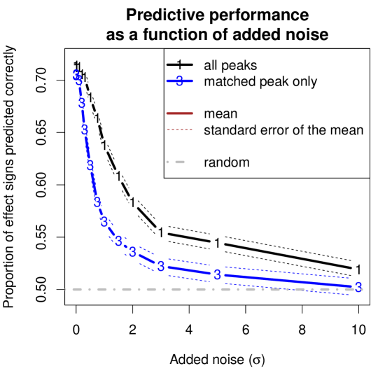
Figure 6: Model 1 yields a better accuracy at the prediction of signs of covariate effects for previously unseen lipids in the lipidomic gene-silencing data set. The difference to Model 3 becomes pronounced when simulated noise is added to the data. The prediction is based on the inferred covariate effects of compounds from the same lipid family and is done in a cross-validation setting. In the task, the effects of the seven gene-silencing treatments are predicted on the three most abundant families of lipids in two time points. Points $\sigma=0$ and $\sigma>0$ on the x-axis show the prediction accuracy (y-axis) for the original data and the data with added noise, respectively.

3.3.3 Robustness of effect magnitudes

To evaluate the inferred effects at the scale of the entire observed lipidome, we examine the consistency of inferred covariate effects between the original and noise-added data sets. This experiment simulates the situation where the true effects are known (effects from the original data set), but the data based on which the effects are inferred are noisy (the added-noise data set). To measure the consistency, we compute the Spearman correlation between the covariate effects inferred from the original and the added-noise data sets for all clusters with two or more peaks.

Model 1 proves more consistent than Model 3 at all noise levels (Figure 7). The confidence intervals from the 100 randomizations do not overlap at all at moderate levels of noise. This gives indication that for a typical biological data set, there is clear benefit from the analysis of multiple peaks, leading to reduced variance of the result.

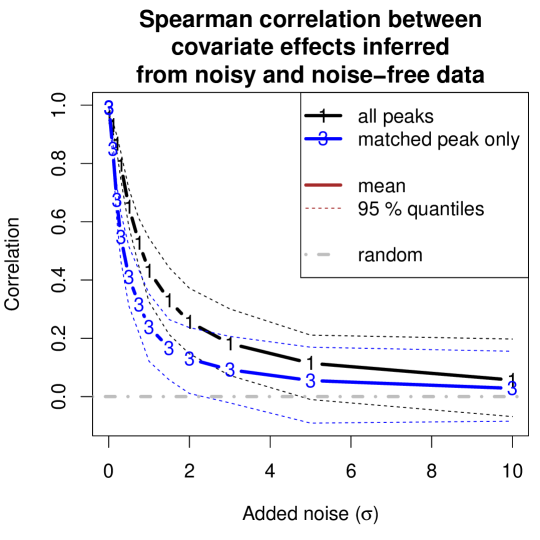
Figure 7: The covariate effects inferred by Model 1 are more robust to noise compared to Model 3. At moderate levels of noise, which is the regime of many biological experiments, the confidence intervals over 100 randomizations do not overlap at all. The robustness is quantified as the Spearman correlation (y-axis) between the effects inferred from the noisy and noise-free versions of the lipidomic gene silencing data set as a function of the level of noise (x-axis).

3.3.4 Stability

As the proposed approach is sensitive to the inferred clustering of the data, we analyze the stability of the inferred clustering on biological data, using the lipidomic gene silencing data as a case. We test the influence of the concentration parameter $\alpha_{\text{DP}}$ in the Dirichlet process clustering model. The clustering result for the lipidomic gene silencing data turns out to be very robust to changes in the magnitude of the concentration parameter (Figure 2 in Supplementary material). As expected, the number of clusters increases as the preset value of the concentration parameter increases but the relative change is small. Also the change in the consistency of the learned covariate effects is small.

3.3.5 Qualitative analysis

Finally, we give concrete examples of potential findings that the approaches can uncover and demonstrate how analysis based on a single peak may lead to a different outcome depending on the choice of the peak.

The intervention-driven changes of individual peaks from two lipids along with the covariate effects inferred by Models 1 and 3 are shown in Figure 8. In the case of the sphingomyelin SM(d18:1/22:0), there are strong covariate effects inferred by Model 3 but many of these effects become weaker when inferred based on multiple peaks by Model 1. On the contrary, Model 3 infers weak covariate effects for the ceramide Cer(d18:1/17:0) but based on multiple peaks and Model 1, one of the effects is actually among the top-5 % strongest effects across the observed lipidome. These examples underline the fact that conclusions based on mass spectral data are highly sensitive to the choice of peak, but the variance therein can be reduced by model-based integration of data from multiple associated peaks.

Figure 8: Example clusters of peaks from the lipidomic gene silencing data with differences in the covariate effects inferred based on a single peak and multiple peaks. There is noticeable variation between peaks associated with one compound. The choice of the representative peak thus affects the inferred covariate effects. The heat maps show changes in the lipid concentrations driven by the gene silencing interventions (columns). Covariate effects inferred by Models 3 and 1 using a single peak and all peaks, respectively, are shown on the two bottom rows of each heat map. The $\log_{2}$ fold changes of each peak associated with the compound are shown on the top rows. Changes that by the magnitude fall to the top-5 % across the entire observed lipidome are highlighted by the symbol ”T.“ Top (a): The sphingomyelin SM(d18:1-22:0) with three peaks. Many strong changes for SM(d18:1-22:0) become weaker when they are inferred based on all three peaks. Bottom (b): The ceramide Cer(d18:1-17:0) with six peaks. The effect of the SCAP silencing for Cer(d18:1-17:0) at 72 hours becomes strong when it is inferred based on all six peaks.

4 Conclusion

We have empirically demonstrated that a model-based integration of multiple peaks can lead to an improved accuracy in the inference of covariate effects, and introduced a novel method for this task. While the sample-size is always restricted by external constraints such as the experiment budget or the availability of suitable patients, the inference based on multiple peaks gives a shortcut to extracting more information from the limited set of samples, thereby directly addressing the “small $n$, large $p$” problem. However, some types of systematic measurement error, such as some batch effects, escape this treatment and can only be reduced by introducing independent replicates. In this work, we have shown that additional peaks are especially useful when the signal-to-noise ratio is low and the differences between sample groups are small.

Mass spectral data are noisy to the extent that analysis of small sample-size data sets based on individual spectral peaks is unreliable. The result of this work indicates that additional peaks are useful to the analysis by increasing the accuracy of the inferred covariate effects and by reducing the variance in the estimates. Moreover, the result highlights the risk of relying on a single peak in the comparative analysis of profiles and especially in biomarker discovery. As demonstrated, the inferred covariate effects may change drastically depending on the peak used, when relying on a single peak in the analysis.

We suggest that all the detected peaks that can be associated with a compound should be taken into account in the comparative analysis. This is possible through the two-step generative modeling approach presented in this work: (1) the identification of peaks that can be associated with one compound by clustering the peaks based on their shape similarity and (2) the inference of covariate effects on the clusters, each representing one compound.

References

- [1] Y. Benjamini and Y. Hochberg. Controlling the false discovery rate: a practical and powerful approach to multiple testing. J Roy Stat Soc B Met, 57(1):289–300, 1995.
- [2] J. Boccard, A. Kalousis, M. Hilario, P. Lantéri, M. Hanafi, G. Mazerolles, J.-L. Wolfender, P.-A. Carrupt, and S. Rudaz. Standard machine learning algorithms applied to UPLC-TOF/MS metabolic fingerprinting for the discovery of wound biomarkers in Arabidopsis thaliana. Chemometr Intell Lab, 104(1):20–27, 2010.
- [3] S. Böcker, M. C. Letzel, Z. Lipták, and A. Pervukhin. SIRIUS: decomposing isotope patterns for metabolite identification. Bioinformatics, 25(2):218–224, 2009.
- [4] D. B. Dahl. Bayesian Inference for Gene Expression and Proteomics, chapter Model-based clustering for expression data via a Dirichlet process mixture model, pages 201–218. Cambridge University Press, Cambridge, 2006.
- [5] W. B. Dunn and D. I. Ellis. Metabolomics: current analytical platforms and methodologies. TrAC-Trend Anal Chem, 24(4):285–294, 2005.
- [6] M. D. Escobar. Estimating normal means with a Dirichlet process prior. J Am Stat Assoc, 89(425):268–277, 1994.
- [7] P. Franceschi, D. Masuero, U. Vrhovsek, F. Mattivi, and R. Wehrens. A benchmark spike-in data set for biomarker identification in metabolomics. J Chemometr, 26(1-2):16–24, 2012.
- [8] M. Heinonen, H. Shen, N. Zamboni, and J. Rousu. Metabolite identification and molecular fingerprint prediction through machine learning. Bioinformatics, 28(18):2333–2341, 2012.
- [9] M. Hilvo, C. Denkert, L. Lehtinen, B. Müller, S. Brockmöller, T. Seppänen-Laakso, J. Budczies, E. Bucher, L. Yetukuri, S. Castillo, E. Berg, H. Nygren, M. Sysi-Aho, J. Griffin, O. Fiehn, S. Loibl, C. Richter-Ehrenstein, C. Radke, T. Hyötyläinen, O. Kallioniemi, K. Iljin, and M. Orešič. Novel theranostic opportunities offered by characterization of altered membrane lipid metabolism in breast cancer progression. Cancer Res, 71(9):3236–3245, 2011.
- [10] N. Huang, M. M. Siegel, G. H. Kruppa, and F. H. Laukien. Automation of a Fourier transform ion cyclotron resonance mass spectrometer for acquisition, analysis, and e-mailing of high-resolution exact-mass electrospray ionization mass spectral data. J Am Soc Mass Spectr, 10(11):1166–1173, 1999.
- [11] I. Huopaniemi, T. Suvitaival, J. Nikkilä, M. Orešič, and S. Kaski. Two-way analysis of high-dimensional collinear data. Data Min Knowl Disc, 19(2):261–276, 2009.
- [12] T. Kind and O. Fiehn. Metabolomic database annotations via query of elemental compositions: mass accuracy is insufficient even at less than 1 ppm. BMC Bioinformatics, 7(1):234, 2006.
- [13] T. J. Mitchell and J. J. Beauchamp. Bayesian variable selection in linear regression. J Am Stat Assoc, 83(404):1023–1032, 1988.
- [14] M. Orešič, V. A. Hänninen, and A. Vidal-Puig. Lipidomics: a new window to biomedical frontiers. Trends Biotechnol, 26(12):647–652, 2008.
- [15] T. Pluskal, S. Castillo, A. Villar-Briones, and M. Orešič. MZmine 2: modular framework for processing, visualizing, and analyzing mass spectrometry-based molecular profile data. BMC Bioinformatics, 11(1):395, 2010.
- [16] S. Rogers, R. Daly, and R. Breitling. Mixture model clustering for peak filtering in metabolomics. In A. Larjo, S. Schober, M. Farhan, M. Bossert, and O. Yli-Harja, editors, Ninth International Workshop on Computational Systems Biology, WCSB 2012, June 4-6, 2012, Ulm, Germany, number 61 in TICSP series, pages 71–74, Tampere, 2012. Tampere University of Technology.
- [17] A. Scalbert, L. Brennan, O. Fiehn, T. Hankemeier, B. S. Kristal, B. van Ommen, E. Pujos-Guillot, E. Verheij, D. Wishart, and S. Wopereis. Mass-spectrometry-based metabolomics: limitations and recommendations for future progress with particular focus on nutrition research. Metabolomics, 5(4):435–458, 2009.
- [18] A. Shevchenko and K. Simons. Lipidomics: coming to grips with lipid diversity. Nat Rev Mol Cell Bio, 11(8):593–598, 2010.
- [19] C. A. Smith, E. J. Want, G. O’Maille, R. Abagyan, and G. Siuzdak. XCMS: processing mass spectrometry data for metabolite profiling using nonlinear peak alignment, matching, and identification. Anal Chem, 78(3):779–787, 2006.
- [20] R. Steuer. Review: on the analysis and interpretation of correlations in metabolomic data. Brief Bioinform, 7(2):151–158, 2006.
- [21] N. Vinh, J. Epps, and J. Bailey. Information theoretic measures for clusterings comparison: variants, properties, normalization and correction for chance. J Mach Learn Res, 11:2837–2854, 2010.
- [22] W. Windig, J. M. Phalp, and A. W. Payne. A noise and background reduction method for component detection in liquid chromatography/mass spectrometry. Anal Chem, 68(20):3602–3606, 1996.