Discrete-event simulation of uncertainty in single-neutron experiments

Abstract

A discrete-event simulation approach which provides a cause-and-effect description of many experiments with photons and neutrons exhibiting interference and entanglement is applied to a recent single-neutron experiment that tests (generalizations of) Heisenberg’s uncertainty relation. The event-based simulation algorithm reproduces the results of the quantum theoretical description of the experiment but does not require the knowledge of the solution of a wave equation nor does it rely on concepts of quantum theory. In particular, the data satisfies uncertainty relations derived in the context of quantum theory.

I Introduction

Quantum theory has proven extraordinarily powerful for describing a vast number of laboratory experiments. The mathematical framework of quantum theory allows for a straightforward (at least in principle) calculation of numbers which can be compared with experimental data as long as these numbers refer to statistical averages of measured quantities, such as for example atomic spectra, the specific heat and magnetic susceptibility of solids. However, as soon as an experiment is able to record the individual clicks of a detector which contribute to the statistical average a fundamental problem appears. Although quantum theory provides a recipe to compute the frequencies for observing events, it does not account for the observation of the individual events themselves (Ballentine, 1970; Home, 1997; Ballentine, 2003; Allahverdyan et al., 2013). Prime examples are the single-electron two-slit experiment (Tonomura, 1998), single-neutron interferometry experiments (Rauch and Werner, 2000) and optics experiments in which the click of a detector is assumed to correspond to the arrival of a single photon (Garrison and Chiao, 2008).

From the viewpoint of quantum theory, the central issue is how it can be that experiments yield definite answers. On the other hand, it is our brain which decides, based on what it perceives through our senses and cognitive capabilities, what a definite answer is and what it is not. According to Bohr (Bohr, 1999) “Physics is to be regarded not so much as the study of something a priori given, but rather as the development of methods of ordering and surveying human experience. In this respect our task must be to account for such experience in a manner independent of individual subjective judgment and therefore objective in the sense that it can be unambiguously communicated in ordinary human language”. This quote may be read as a suggestion to construct a description in terms of events, some of which are directly related to human experience, and the cause-and-effect relations among them. Such an event-based description obviously yields definite answers and if it reproduces the statistical results of experiments, it also provides a description on a level to which quantum theory has no access.

For many interference and entanglement phenomena observed in optics and neutron experiments, such an event-based description has already been constructed, see  (Michielsen et al., 2011; De Raedt and Michielsen, 2012; De Raedt et al., 2012a) for recent reviews. The event-based simulation models reproduce the statistical distributions of quantum theory without solving a wave equation but by modeling physical phenomena as a chronological sequence of events. Hereby events can be actions of an experimenter, particle emissions by a source, signal generations by a detector, interactions of a particle with a material and so on (Michielsen et al., 2011; De Raedt and Michielsen, 2012; De Raedt et al., 2012a).

The basic premise of our event-based simulation approach is that current scientific knowledge derives from the discrete events which are observed in laboratory experiments and from relations between those events. Hence, the event-based simulation approach is concerned with how we can model these experimental observations but not with what “really” happens in Nature. This underlying premise strongly differs from the assumption that the observed events are signatures of an underlying objective reality which is mathematical in nature but is in line with Bohr’s viewpoint expressed in the above quote.

The general idea of the event-based simulation method is that simple rules define discrete-event processes which may lead to the behavior that is observed in experiments. The basic strategy in designing these rules is to carefully examine the experimental procedure and to devise rules such that they produce the same kind of data as those recorded in experiment, while avoiding the trap of simulating thought experiments that are difficult to realize in the laboratory. Evidently, mainly because of the lack of knowledge, the rules are not unique. Hence, it makes sense to use the simplest rules one could think of until a new experiment indicates that the rules should be modified. The method may be considered as entirely “classical” since it only uses concepts which are directly related to our perception of the macroscopic world but the rules themselves are not necessarily those of classical Newtonian dynamics.

The event-based approach has successfully been used for discrete-event simulations of quantum optics experiments such as the single beam splitter and Mach-Zehnder interferometer experiments, Wheeler’s delayed choice experiments, a quantum eraser experiment, two-beam single-photon interference experiments and the single-photon interference experiment with a Fresnel biprism, Hanbury Brown-Twiss experiments, Einstein-Podolsky-Rosen-Bohm (EPRB) experiments, and of conventional optics problems such as the propagation of electromagnetic plane waves through homogeneous thin films and stratified media, see (Michielsen et al., 2011; De Raedt and Michielsen, 2012) and references therein. For applications to single-neutron interferometry experiments see (De Raedt and Michielsen, 2012; De Raedt et al., 2012a). The same methodology has also been employed to perform discrete-event simulations of quantum cryptography protocols (Zhao and De Raedt, 2008) and universal quantum computation (Michielsen et al., 2005).

In this paper, we extend this list by demonstrating that the same approach provides an event-by-event description of recent neutron experiments (Erhart et al., 2012; Sulyok et al., 2013) devised to test (generalizations of) Heisenberg’s uncertainty principle. It is shown that the event-by-event simulation generates data which complies with the quantum theoretical description of this experiment. Therefore, these data also satisfy the inequalities which, in quantum theory, express (generalizations of) Heisenberg’s uncertainty principle. However, as the event-by-event simulation does not resort to concepts of quantum theory these findings indicate that there is little intrinsically “quantum mechanical” to these inequalities, in concert with the idea that quantum theory can be cast into a “classical” statistical theory (Frieden, 1989; Reginatto, 1998; Hall, 2000; Frieden, 2004; Khrennikov, 2009, 2011; Khrennikov et al., 2011; Kapsa et al., 2010; Skála et al., 2011; Kapsa and Skála, 2011; Klein, 2012, 2010; Flego et al., 2012).

II Experiment and quantum theoretical description

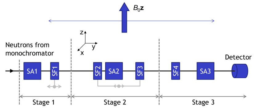
Figure 1: Functional block diagram of the neutron experiment (Erhart et al., 2012; Sulyok et al., 2013) to test uncertainty relations, see also Fig. 2 in (Erhart et al., 2012; Sulyok et al., 2013). Monochromatic neutrons enter from the left. SA1, SA2, SA3: spin analyzers (see text); SF1, SF2, SF3, SF4: spin flippers (see text). The positions of SF1 and the pair (SF2,SF3) are variable. The preparation stage 1 manipulates the magnetic moments of the neutrons such that, depending on the orientation of SA1 and the position of SF1, they leave stage 1 with their moments directed along the $z$-axis or along a fixed direction on the $x-y$ plane. In the quantum theoretical description (see text), stage 2 and stage 3 perform the successive measurement of the eigenvalues of the spin operators $\sigma_{\phi}=\sigma_{x}\cos\phi+\sigma_{y}\sin\phi$ and $\sigma_{y}$, respectively. These seven devices, in combination with the static magnetic field $B_{0}\mathbf{z}$ and the variable positions of SF1 and (SF2,SF3), are sufficient to determine the expectation values that appear in Heisenberg-like uncertainty relations (see text).

A block diagram of the neutron experiment designed to test uncertainty relations (Erhart et al., 2012; Sulyok et al., 2013) is shown in Fig. 1. We now describe this experiment in operational terms and as we go along, we also give the quantum theoretical description in terms of spin 1/2 particles such as neutrons.

Conceptually, the neutron experiment (Erhart et al., 2012; Sulyok et al., 2013) exploits two different physical phenomena: the motion of a magnetic moment in a static magnetic field and a spin-analyzer that performs a Stern-Gerlach-like selection of the neutrons based on the direction of their magnetic moments.

A magnetic moment $\mathbf{S}$ in an external, static magnetic field $B\mathbf{e}$ experiences a rotation about the direction of the unit vector $\mathbf{e}$. The unitary transformation that corresponds to such a rotation is given by

$$U_{\mathbf{b}}(\varphi) = e^{i\gamma tB\mathbf{S}\cdot\mathbf{e}}=e^{i\varphi{\bm{\sigma}}\cdot\mathbf{e}},$$ (1)

where $\gamma$ is the gyromagnetic ration of the particle, $t$ is the time that the particle interacts with the magnetic field, the variable $\varphi=\gamma tB$ is introduced as a shorthand for the angle of rotation, and ${\bm{\sigma}}=(\sigma_{x},\sigma_{y},\sigma_{z})$ denote the Pauli-spin matrices.

The spin analyzer acts as a projector. It is a straightforward (see pages 172 and 250 in (Ballentine, 2003)) to show that within quantum theory, an ideal spin analyzer directed along the unit vector ${\mathbf{n}}$ is represented by the projection operator

$$M(S,\bm{n}) = \frac{\leavevmode\hbox{\small 1\normalsize\kern-3.30002pt1}+S{\bm{\sigma}}\cdot\mathbf{n}}{2},$$ (2)

where 11 is the unit matrix and $S=\pm 1$ selects one of the two possible alignments of the spin polarizer along ${\mathbf{n}}$ (see (Erhart et al., 2012; Sulyok et al., 2013)).

Using Eqs. (1) and (2), it is straightforward to construct the quantum theoretical description of each of the three stages in the experimental setup.

1. The purpose of the first spin analyzer (SA1) is to prepare neutrons with their magnetic moments in the direction of the static magnetic field $B_{0}\bm{z}$. Then, the particle travels for some time in a region where the field $B_{0}\bm{z}$ is present but as its magnetic moment is aligned along $z$, the magnetic moment does not rotate.

   As will become clear later, to test Ozawa’s inequality (Ozawa, 2003; Erhart et al., 2012; Sulyok et al., 2013), it is necessary to be able to prepare initial states in which the magnetic moment lies in the $x-y$ plane. In the experiment, this is accomplished by putting in place, the spin flipper SF1. The spin flipper (SF1), in essence a static magnetic field aligned along the $x$-direction, rotates the magnetization about the $x$-axis by an amount proportional to the magnetic field. For simplicity, it is assumed that this rotation changes the direction of the magnetic moment from $z$ to $y$ (Erhart et al., 2012; Sulyok et al., 2013). The position of SF1, relative to the direction of flight of the neutrons, is variable. By moving SF1 one can change the time that the particles perform rotations about the $z$-axis, hence one can control the direction of the magnetic moment in the $x-y$ plane as it leaves stage 1.

   Quantum theoretically, the action of the components of stage 1 is described by the product of unitary matrices

   $$U_{1} = U_{\mathbf{z}}(\theta_{1})U_{\mathbf{x}}(\theta_{0}),$$ (3)

   where $\theta_{0}=\pi/2$ or $\theta_{0}=0$ if SF1 is in place or not and $\theta_{1}$ is the variable (through the variable position of SF1) rotation angle, the value of which will be fixed later. Obviously, in the case that SF1 is not present, because the incoming neutrons have their moments aligned along the $z$-direction, these moments do not perform rotations at all.

2. This stage consists of a pair of spin flippers (SF2,SF3) and a spin analyzer (SA2). The position of (SF2,SF3), relative to the direction of flight of the neutrons, is variable whereas the position of SA2 is fixed. The action of the components of stage 2 is described by the product of matrices

   $$T_{2} = U_{\mathbf{z}}(\theta_{4})U_{\mathbf{x}}(\pi/2)M(S_{1},\bm{z})U_{\mathbf{z}}(\theta_{3})U_{\mathbf{x}}(\pi/2)U_{\mathbf{z}}(\theta_{2}),$$ (4)

   where, as a consequence of the variable position of (SF2,SF3), the rotation angles $\theta_{2}$, $\theta_{3}$, and $\theta_{4}$ change with the position of (SF2,SF3). The value of variable $S_{1}=\pm 1$ labels one of the two possible alignments of the spin polarizer along $\mathbf{z}$. Note that because of the projection $M(S_{1},\bm{z})$, the matrix $T_{2}$ is not unitary.

3. The final stage consists of a spin flipper SF4 and a spin analyzer SA3. The time evolution of the magnetic moment as it traverses this stage is given by

   $$T_{3} = M(S_{2},\bm{z})U_{\mathbf{z}}(\theta_{5})U_{\mathbf{x}}(\pi/2),$$ (5)

   where $\theta_{5}$ is a fixed rotation angle. The value of variable $S_{2}=\pm 1$ labels one of the two possible alignments of the spin polarizer along $\mathbf{z}$. The matrix $T_{3}$ is not unitary.

According to the postulates of quantum theory, the probability to detect a neutron leaving stage 3 is given by (Ballentine, 2003)

$$P(S_{1},S_{2}|\rho) = \mathbf{Tr}\rho(T_{3}T_{2}U_{1})^{\dagger}(T_{3}T_{2}U_{1}),$$ (6)

where it is assumed that the detector simply counts every impinging neutron (which in view of the very high detection efficiency is a very good approximation, see  (Rauch and Werner, 2000)). In Eq. (6), the initial state of the S=1/2 quantum system is represented by the density matrix

$$\rho = \frac{\leavevmode\hbox{\small 1\normalsize\kern-3.30002pt1}+{\bm{\sigma}}\cdot\mathbf{a}}{2}.$$ (7)

The real-valued vector $\mathbf{a}$ ($\|\mathbf{a}\|\leq 1$) completely determines the initial state of the quantum system. Using Eq. (3) – (7) we find

$$P(S_{1},S_{2}|\mathbf{a}) = \frac{1+(S_{1}-S_{2}\cos\theta_{4})(a_{x}\sin(\theta_{1}+\theta_{2})-a_{y}\cos(\theta_{1}+\theta_{2}))-S_{1}S_{2}\cos\theta_{4}}{4},$$ (8)

independent of $\theta_{3}$ and $\theta_{5}$. Recall that by construction of the experimental setup $\theta_{2}+\theta_{4}$ is fixed. We can make contact to the expressions used in the analysis of the neutron experiment (Erhart et al., 2012; Sulyok et al., 2013), by substituting $\theta_{1}=0$, $\theta_{2}=\phi+\pi/2$ and $\theta_{4}=-\phi-\pi/2$ where $\phi$ is called the detuning angle (Erhart et al., 2012; Sulyok et al., 2013). We obtain

$$P(S_{1},S_{2}|\mathbf{a}) = \frac{1+(S_{1}+S_{2}\sin\phi)(a_{x}\cos\phi+a_{y}\sin\phi)+S_{1}S_{2}\sin\phi}{4}.$$ (9)

As explained in detail in subsection II.1, the experimental setup can be interpreted as performing successive measurements of the operators $\sigma_{\phi}=\sigma_{x}\cos\phi+\sigma_{y}\sin\phi$ and $\sigma_{y}$, their eigenvalues being $S_{1}$ and $S_{2}$, respectively. Note that these two operators do not commute unless $\cos\phi=0$ and that the observed eigenvalues $S_{1}$ and $S_{2}$ of these two operators are correlated, as is evident from the contribution $S_{1}S_{2}\sin\phi$ in Eq. (9).

From Eq. (9), the expectation values of the various spin operators follow immediately. Specifically, we have

$$\langle\sigma_{\phi}\rangle_{\mathbf{a}} = \sum_{S_{1},S_{2}=\pm 1}S_{1}P(S_{1},S_{2}|\mathbf{a})=a_{x}\cos\phi+a_{y}\sin\phi,$$

$$\langle\sigma_{y}\rangle_{\mathbf{a}} = \sum_{S_{1},S_{2}=\pm 1}S_{2}P(S_{1},S_{2}|\mathbf{a})=\sin\phi(a_{x}\cos\phi+a_{y}\sin\phi)=\sin\phi\langle\sigma_{\phi}\rangle_{\mathbf{a}},$$ (10)

and as $\sigma_{\phi}^{2}=\sigma_{y}^{2}=1$, the variances $\langle\sigma_{\phi}^{2}\rangle_{\mathbf{a}}-\langle\sigma_{\phi}\rangle_{\mathbf{a}}^{2}$ and $\langle\sigma_{y}^{2}\rangle_{\mathbf{a}}-\langle\sigma_{y}\rangle_{\mathbf{a}}^{2}$ are completely determined by Eq. (10).

II.1 Filtering-type measurements of one spin-1/2 particle

The neutron experiment (Erhart et al., 2012; Sulyok et al., 2013) can be viewed as a particular realization of a filtering-type experiment (Ballentine, 2003; De Raedt et al., 2011). The layout of such an experiment is shown in Fig. 2. According to this diagram, the experiment consists of performing successive Stern-Gerlach-type measurements on one spin-1/2 particle at a time. Conceptually, assuming a stationary particle source, the neutron experiment (Erhart et al., 2012; Sulyok et al., 2013) and the filtering-type experiment shown in Fig. 2 are identical, see also Fig. 1 in (Erhart et al., 2012; Sulyok et al., 2013). In practice, the difference between the filtering-type experiment and the neutron experiment (Erhart et al., 2012; Sulyok et al., 2013) is that in the latter four experiments (labeled by the variables $S_{1}=\pm 1$ and $S_{2}=\pm 1$), are required for each of the two opposite orientations of the two spin analyzers SA2 and SA3 whereas the setup depicted in Fig. 2 directly yields the results of the four separate runs.

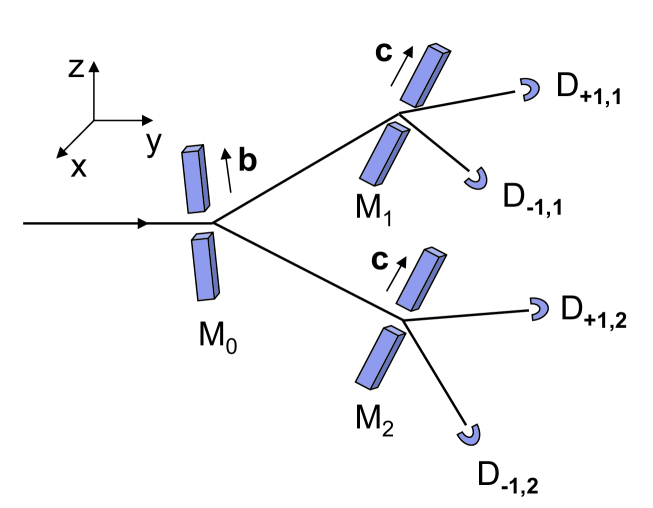
Figure 2: Diagram of the filtering-type experiment of which the neutron experiment (Erhart et al., 2012; Sulyok et al., 2013) is a special case. Spin-1/2 particles pass through a Stern-Gerlach magnet $M_{0}$ that projects the spin onto either the ${\mathbf{b}}$ direction or the $-{\mathbf{b}}$ direction. In case of the former (latter) projection, the particle is directed to the Stern-Gerlach magnet $M_{1}$ ($M_{2}$). $M_{1}$ and $M_{2}$ are assumed to be identical and project the spin onto either the ${\mathbf{c}}$ direction or the $-{\mathbf{c}}$ direction. A “click” of one of the four detectors $D_{+1,1}$, $D_{-1,1}$, $D_{+1,2}$, and $D_{-1,2}$ signals the arrival of a particle.

The pictorial description of the filtering experiment goes as follows. A particle enters the Stern-Gerlach magnet $M_{0}$, with its magnetic field along direction ${\mathbf{b}}$. $M_{0}$ “sends” the particle either to Stern-Gerlach magnet $M_{1}$ or $M_{2}$. The magnets $M_{1}$ and $M_{2}$, identical and both with their magnetic field along direction ${\mathbf{c}}$, redirect the particle once more and finally, the particle is registered by one of the four detectors $D_{+1,1}$, $D_{-1,1}$, $D_{+1,2}$, and $D_{-1,2}$. This scenario is repeated until the statistical fluctuations of the counts of the four detectors are considered to be sufficiently small.

We label the particles by a subscript $\alpha$. After the $\alpha$th particle leaves $M_{1}$ or $M_{2}$, it will hit one (but only one) of the four detectors. We assume ideal experiments, that is at any time one and only one out of four detectors fires. We write $x_{\alpha}^{(i,j)}=1$ with $i=\pm 1$ and $j=1,2$ if the $\alpha$th particle was detected by detector $D_{i,j}$ and $x_{\alpha}^{(i,j)}=0$ otherwise.

We define two new dichotomic variables by

$$S_{1,\alpha} = \left(x_{\alpha}^{(+1,1)}+x_{\alpha}^{(-1,1)}\right)-\left(x_{\alpha}^{(+1,2)}+x_{\alpha}^{(-1,2)}\right),$$

$$S_{2,\alpha} = \left(x_{\alpha}^{(+1,1)}+x_{\alpha}^{(+1,2)}\right)-\left(x_{\alpha}^{(-1,1)}+x_{\alpha}^{(-1,2)}\right).$$ (11)

Note that for each incoming particle, only one of the detectors clicks hence only one of the $x_{\alpha}^{(i,j)}$’s is nonzero or, equivalently $x_{\alpha}^{(+1,1)}+x_{\alpha}^{(-1,1)}+x_{\alpha}^{(+1,2)}+x_{\alpha}^{(-1,2)}=1$.

In the quantum theoretical description of the filtering experiment, if $S_{1,\alpha}=\pm 1$, the spin has been projected on the $\pm{\mathbf{b}}$ direction. Likewise, if $S_{2,\alpha}=\pm 1$, the spin has been projected on the $\pm{\mathbf{c}}$ direction. In other words, $S_{1,\alpha}$ and $S_{2,\alpha}$ are the eigenvalues of the spin operator projected on the directions ${\mathbf{b}}$ and ${\mathbf{c}}$, respectively. Then, according to quantum theory, the probability to observe a pair of eigenvalues $(S_{1},S_{2})$ is given by (Ballentine, 2003; De Raedt et al., 2011)

$$P(S_{1},S_{2}|\mathbf{a}) = \mathbf{Tr}\rho\left(M(S_{2},{\mathbf{c}})M(S_{1},{\mathbf{b}})\right)^{\dagger}\left(M(S_{2},{\mathbf{c}})M(S_{1},{\mathbf{b}})\right)$$ (12)

$$= \mathbf{Tr}\rho M(S_{1},\mathbf{b})M(S_{2},{\mathbf{c}})M(S_{1},{\mathbf{b}})$$

$$= \frac{1+(S_{1}+\mathbf{b}\cdot\mathbf{c}\;S_{2})\mathbf{a}\cdot\mathbf{b}+\mathbf{b}\cdot\mathbf{c}\;S_{1}S_{2}}{4},$$

where the state $\rho$ is given by Eq. (7) and the $M$’s denote projection operators. It is easy to see that Eq. (9) is a particular case of Eq. (12).

Note that $[M(S_{1},{\mathbf{b}}),M(S_{2},{\mathbf{c}})]\not=0$ unless $\mathbf{b}=\pm\mathbf{c}$, $[\rho,M(S_{1},{\mathbf{b}})]\not=0$ unless $\mathbf{a}=\pm\mathbf{b}$, and that $[\rho,M(S_{2},{\mathbf{c}})]\not=0$ unless $\mathbf{a}=\pm\mathbf{c}$. Thus, for virtually all cases of interest, none of the operators in Eq. (12) commute, yet quantum theory yields the probability $P(S_{1},S_{2}|\mathbf{a})$ for all cases. Clearly, the statement that one can determine the eigenvalues of two non-commuting operators in one experiment contradicts the conventional teaching that non-commuting operators cannot be diagonalized simultaneously and therefore cannot be measured simultaneously. The reason for this apparent contradiction is the hidden assumption that diagonalization and the act of measurement in a laboratory (i.e. a click of the detector) are equivalent in some sense. The filtering-type experiment is a clear example which shows that they are not: according to quantum theory the eigenvalues $S_{1}$ and $S_{2}$ of the operators ${\bm{\sigma}}\cdot\mathbf{b}$ and ${\bm{\sigma}}\cdot\mathbf{c}$, respectively can always be measured simultaneously even though these operators cannot always be diagonalized simultaneously.

III Event-by-event simulation

A minimal, discrete-event simulation model of single-neutron experiments requires a specification of the information carried by the neutrons, of the algorithm that simulates the source and the devices used in the experimental setup (see Fig. 1), and of the procedure to analyze the data.

• Messenger: A neutron is regarded as a messenger carrying a message. In principle, there is a lot of freedom to specify the content of the message, the only criterion being that in the end, the simulation should reproduce the results of real laboratory experiments. We adopt Occam’s razor as a guiding principle to determine which kind of data the messenger should carry with it, that is we use the minimal amount of data.

  The pictorial description that will be used in the following should not be taken literally: it is only meant to help visualize, in terms of concepts familiar from macroscopic physics, the minimal amount of data the messenger should carry.

  Picturing the neutron as a tiny classical magnet we can use the spherical coordinates $\theta$ and $\varphi$ to specify the direction of its magnetic moment

  $${\mathbf{m}}=(\cos\varphi\sin\theta,\sin\varphi\sin\theta,\cos\theta)^{T},$$ (13)

  relative to the fixed frame of reference defined by the static magnetic field $B_{0}\mathbf{z}$. The messenger should also be aware of the time it takes to move from one point in space to another. The time of flight and the direction of the magnetic moment are conveniently encoded in a message of the type (De Raedt and Michielsen, 2012; De Raedt et al., 2012a)

  $${\mathbf{u}}=(e^{i\psi^{(1)}}\cos(\theta/2),e^{i\psi^{(2)}}\sin(\theta/2))^{T},$$ (14)

  where $\psi^{(i)}=\nu t+\delta_{i}$, for $i=1,2$ and $\varphi=\delta_{1}-\delta_{2}=\psi^{(1)}-\psi^{(2)}$. Within the present model, the state of the neutron, that is the message, is completely described by the angles $\psi^{(1)}$, $\psi^{(2)}$ and $\theta$ and by rules (to be specified), by which these angles change as the neutron travels through the network of devices. This model suffices to reproduce the results of single-neutron interference and entanglement experiments and of their idealized quantum theoretical descriptions (De Raedt and Michielsen, 2012; De Raedt et al., 2012a).

  In specifying the message Eq. (14), we exploited the isomorphism between the algebra of Pauli matrices and rotations in three-dimensional space, not because the former connects to quantum mechanics but only because we find this representation most convenient for our simulation work (Michielsen et al., 2011; De Raedt and Michielsen, 2012; De Raedt et al., 2012a). The direction of the magnetic moment follows from Eq. (14) through

  $${\mathbf{m}}={\mathbf{u}}^{T}{\bm{\sigma}}{\mathbf{u}}.$$ (15)

  A messenger with message ${\mathbf{u}}$ at time $t$ and position ${\mathbf{r}}$ that travels with velocity $v$, along the direction ${\mathbf{q}}$ during a time interval $t^{\prime}-t$, changes its message according to $\psi^{(i)}\leftarrow\psi^{(i)}+\nu(t^{\prime}-t)$ for $i=1,2$, where $\nu$ is an angular frequency which is characteristic for a neutron that moves with a fixed velocity $v$. In a monochromatic beam of neutrons, all neutrons have the same value of $\nu$ (Rauch and Werner, 2000).

  In the presence of a magnetic field ${\mathbf{B}}=(B_{x},B_{y},B_{z})$, the magnetic moment rotates about the direction of ${\mathbf{B}}$ according to the classical equation of motion

  $$\frac{d\mathbf{m}}{dt}=\mathbf{m}\times{\mathbf{B}}.$$ (16)

  Hence, as the messenger passes a region in which a magnetic field is present, the message ${\mathbf{u}}$ changes into the message

  $${\mathbf{u}}\leftarrow e^{ig\mu_{N}T\mathbf{\sigma}\cdot{\mathbf{B}}/2}{\mathbf{u}},$$ (17)

  where $g$ denotes the neutron $g$-factor, $\mu_{N}$ the nuclear magneton, $T$ the time during which the messenger experiences the magnetic field.

  In the event-based simulation of the experiment shown in Fig. 1, the time-of-flight $T$ determines the angle of rotation of the magnetic moment through Eq. (17) and can, so to speak, be eliminated by expressing all operations in terms of rotation angles. However, this simplification is no longer possible in the event-based simulation of single-neutron interference and entanglement experiments (De Raedt and Michielsen, 2012; De Raedt et al., 2012a).

• Source: When the source creates a messenger, its message needs to be initialized. This means that three angles $\psi^{(1)}$, $\psi^{(2)}$ and $\theta$ need to be specified. In practice, instead of implementing stage 1 it is more efficient to prepare the messengers such that the corresponding magnetic moments are along a specified, fixed direction. For instance, to mimic fully coherent, spin-polarized neutrons that enter stage 2 with their spin along the $x$-axis, the source would create messengers with $\theta=\pi/2$, and without loss of generality, $\psi^{(1)}=\psi^{(2)}=0$.

• Spin-flipper: The spin-flipper rotates the magnetic moment by an angle $\pi/2$ about the $x$ axis.

• Spin analyzer: This device shares with the magnet used in Stern-Gerlach experiments the property that it diverts incoming particles in directions which depend on the orientation of their magnetic moments relative to the magnetic field inside the device. For appropriate choices of the experimental parameters, the Stern-Gerlach magnet splits the incoming beam of particles into spatially separated beams. If there are two well-separated beams, the action of the device its to align the magnetic moments of the incoming particles either parallel or anti-parallel to the direction of the field.

  Ignoring all the details of interaction of the magnetic moments with the Stern-Gerlach magnet, the operation of separating the incoming beam into spatially separated beams is captured by the very simple probabilistic model defined by

  $$x=2\Theta\left(\frac{1+m_{z}S}{2}-r\right)-1,$$ (18)

  where $x=-1,1$ labels the two distinct spatial directions, $0<r<1$ is a uniform pseudo-random number, $\Theta(x)$ is the unit step function and, as before, $S=\pm 1$ labels the orientation of the spin analyzer. For each incoming messenger, a new pseudo-random number is being generated. Recall that $|m_{z}|\leq 1$ (see Eq. (13)) hence the first term of Eq. (18) is a number between zero and two. If we would set $m_{z}=\langle{\bm{\sigma}}\cdot\mathbf{n}\rangle$, the model defined by Eq. (18) would generate minus- and plus ones according to the projection operator Eq. (2). Applied to the neutron experiments (Erhart et al., 2012; Sulyok et al., 2013), the function of the spin analyzer is to pass particles with say, spin-up, only. In the simulation model this translates to letting the messenger pass if $x=1$ and destroy the messenger if $x=-1$.

  It is of interest to explore the possibility whether different models for the spin analyzer can yield averages over many events which cannot be distinguished from the results obtained by employing the probabilistic model Eq. (18). As the extreme opposite to the probabilistic model, we consider a deterministic learning machine (DLM) defined by the update rule

  $$x = 2\Theta\left(m_{z}S-\gamma u\right)-1$$

  $$u \leftarrow \gamma u+(1-\gamma)u,$$ (19)

  where $x=-1,1$ labels the two distinct spatial directions and $-1\leq u\leq 1$ encodes the internal state of the DLM (the equivalent of the seed of the pseudo-random number generator). The parameter $0\leq\gamma<1$ controls the pace at which the DLM learns the value $m_{z}S$. The properties of the time series of $x$’s generated by the rules Eq. (19) have been scrutinized in great detail elsewhere, see  (Michielsen et al., 2011) and references therein. Suffice it to say here that for many events, the average of the $x$’s converges to $m_{z}S$ and that the $x$’s are highly correlated in time.

  Obviously, the DLM-based model is extremely simple and fully deterministic. It may easily be rejected as a viable candidate model by comparing the correlations in experimentally observed time series with those generated by Eq. (19). However, if the experiment only provides data about average quantities, there is no way to rule out the DLM model. Unfortunately, the neutron experiments (Erhart et al., 2012; Sulyok et al., 2013) do not provide the data necessary to reject the DLM model, simply because the spin analyzer passes particles with say, spin-up, only. Hence there is no way to compute time correlations. Although we certainly do not want to suggest that the spin analyzers used in the experiments behave in the extreme deterministic manner as described by Eq. (19), it is of interest to test whether such a simple deterministic model can reproduce the averages computed from quantum theory and also obeys the same uncertainty relations as the genuine quantum theoretical model.

• Detector: As a messenger enters the detector, the detection count is increased by one and the messenger is destroyed. The detector counts all incoming messengers. Hence, we assume that the detector has a detection efficiency of 100%. This is a good model of real neutron detectors which can have a detection efficiency of $99\%$ or more (Kroupa et al., 2000).

• Simulation procedure and data analysis: First, we establish the correspondence between the initial message $\mathbf{u}_{\mathrm{initial}}$ and the description in terms of the density matrix Eq. (7). To this end, we remove all devices from stage 1 and 2 and simply count the number of messages that pass SA3 with $S_{2}=1$, for instance. It directly follows from Eq. (18) that the relative frequency of counts is given by $m_{z}$, the projection of the message onto the $z$-axis. In other words, we would infer from the data that in a quantum theoretical description the $z$-component of the density matrix $a_{z}$ is equal to $m_{z}$. By performing rotations of the original message it follows by the same argument that $\mathbf{a}=\mathbf{m}_{\mathrm{initial}}$.

  For each pair of settings $(S_{1},S_{2})$ of the spin analyzers (SA2,SA3) and each position of the pair of spin flippers (SF2,SF3) represented by a rotation of $\phi$ about the $z$-axis (see Section II), the source sends $N$ messengers through the network of devices shown in Fig. 1. The source only creates a new messenger if (i) the previous messenger has been processed by the detector or (ii) the messenger was destroyed by one of the spin analyzers. In other words, direct communication between messengers is excluded. As a device in the network receives a messenger, it processes the message according to the rules specified earlier and sends the messengers with the new message to the next device in the network. If the device is a spin analyzer, it may happen that the messenger is destroyed. The detector counts all messengers that pass SA3 and destroys these messengers.

  For a sequence of $N$ messengers all carrying the same initial message $\mathbf{a}=\mathbf{m}_{\mathrm{initial}}$, this procedure yields a count $N(S_{1},S_{2}|\mathbf{a})$ (recall that $\phi$ is fixed during each sequence of $N$ events). Repeating the procedure for the four pairs of settings yields the relative frequencies

  $$F(S_{1},S_{2}|\mathbf{a}) = \frac{N(S_{1},S_{2}|\mathbf{a})}{\sum_{S_{1},S_{2}=\pm 1}N(S_{1},S_{2}|\mathbf{a})}.$$ (20)

  Note that the numerator in Eq. (20) is not necessarily equal to $N$ because messengers may be destroyed when they enter a spin analyzer. From Eq. (20) we compute

  $$\langle S_{1}\rangle = \sum_{S_{1},S_{2}=\pm 1}S_{1}F(S_{1},S_{2}|\mathbf{a}),$$ (21)

  $$\langle S_{2}\rangle = \sum_{S_{1},S_{2}=\pm 1}S_{2}F(S_{1},S_{2}|\mathbf{a}),$$ (22)

  $$\langle S_{1}S_{2}\rangle = \sum_{S_{1},S_{2}=\pm 1}S_{1}S_{2}F(S_{1},S_{2}|\mathbf{a}).$$ (23)

• Validation. The event-based model reproduces the results of the quantum theoretical description if, within the usual statistical fluctuations, we find that $F(S_{1},S_{2}|\mathbf{a})\approx P(S_{1},S_{2}|\mathbf{a})$ with $P(S_{1},S_{2}|\mathbf{a})$ given by Eq. (9). This correspondence is most easily established by noting that for fixed $\phi$ and $\mathbf{a}$, the three expectations Eqs. (21)–(23) completely determine Eq. (20) and that, likewise, the quantum theoretical distribution Eq. (9) is completely determined by the expectations Eqs. (21)–(23) with $F(S_{1},S_{2}|\mathbf{a})$ replaced by $P(S_{1},S_{2}|\mathbf{a})$. In other words, for the event-based model to reproduce the results of the quantum theoretical description of the neutron experiment (Erhart et al., 2012; Sulyok et al., 2013), it is necessary and sufficient that the simulation results for Eqs. (21)–(23) are in agreement with the quantum theoretical results (see Eq. (10)) $\langle S_{1}\rangle=a_{x}\cos\phi+a_{y}\sin\phi$, $\langle S_{2}\rangle=\sin\phi\langle S_{1}\rangle$, and $\langle S_{1}S_{2}\rangle=\sin\phi$.

  In Figs. 3 and 4, we present representative results of event-based simulations of the neutron experiment (Erhart et al., 2012; Sulyok et al., 2013), showing that the simulation indeed reproduces the predictions of the quantum theoretical description of the neutron experiment (Erhart et al., 2012; Sulyok et al., 2013). Comparing Figs. 3 and 4, we can only conclude that it does not matter whether the model for the spin analyzers uses pseudo-random numbers (Eq. (18)) or is DLM-based (Eq. (19)).

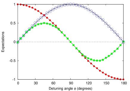
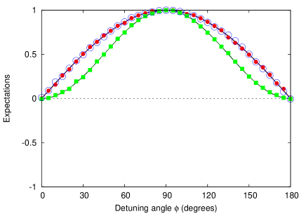
Figure 3: Results for the expectations $\langle S_{1}\rangle$ (red solid circles), $\langle S_{2}\rangle$ (green solid squares), and $\langle S_{1}S_{2}\rangle$ (blue open circles) as obtained by the event-by-event simulation of the neutron experiment (Erhart et al., 2012; Sulyok et al., 2013), using the model Eq. (18) for the spin analyzers. The solid lines represent the corresponding quantum theoretical prediction as obtained from Eq. (9). Left: incoming particles have magnetization $(1,0,0)$. Right: incoming particles have magnetization $(0,1,0)$. For each pair of settings $(S_{1},S_{2})$ of the spin analyzers (SA2,SA3) and each position of the pair of spin flippers (SF2,SF3) represented by a rotation of $\phi$ about the $z$-axis, referred to as detuning angle in (Erhart et al., 2012; Sulyok et al., 2013), the simulation consists of sending $N=10000$ messengers (“neutrons”) into stage 2.

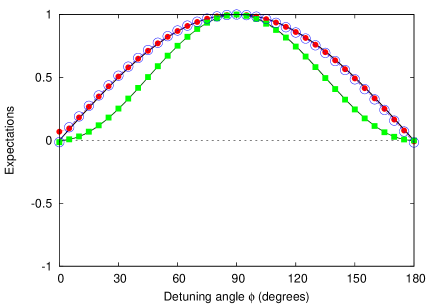
Figure 4: Same as Fig. 3 except that the probabilistic model for the spin-analyzer, as specified by Eq. (18), has been replaced by a deterministic learning machine with an update rule given by Eq. (19). For each pair of settings $(S_{1},S_{2})$ of the spin analyzers (SA2,SA3) and each position of the pair of spin flippers (SF2,SF3) represented by a rotation of $\phi$ about the $z$-axis, referred to as detuning angle in (Erhart et al., 2012; Sulyok et al., 2013), the simulation consists of sending $N=10000$ messengers (“neutrons”) into stage 2. The parameter $\gamma=0.999$.

Summarizing: the event-based simulation model of the neutron experiment (Erhart et al., 2012; Sulyok et al., 2013) presented in this section does not rely, in any sense, on concepts of quantum theory yet it reproduces all features of the quantum theoretical description of the experiment. Although the event-based model is classical in nature, it is not classical in the sense that it cannot be described by classical Hamiltonian dynamics.

IV Uncertainty relations: theory

The neutron experiment (Erhart et al., 2012; Sulyok et al., 2013) was conceived to test an error-disturbance uncertainty relation proposed by Ozawa (Ozawa, 2003). By introducing particular definitions of the measurement error $\epsilon(A)$ of an operator $A$ and the disturbance $\eta(B)$ of an operator $B$, Ozawa showed that

$$\epsilon(A)\eta(B)+\epsilon(A)\Delta(B)+\Delta(A)\eta(B) \geq \frac{1}{2}|\langle[A,B]\rangle|,$$ (24)

where

$$\epsilon^{2}(A) = \langle(M_{A}-A)^{2}\rangle,$$ (25)

$$\eta^{2}(B) = \langle(M_{B}-B)^{2}\rangle,$$ (26)

$$\Delta^{2}(A) = \langle A^{2}\rangle-\langle A\rangle^{2},$$ (27)

$$\Delta^{2}(B) = \langle B^{2}\rangle-\langle B\rangle^{2},$$ (28)

and $M_{A}$ and $M_{B}$ represent the operators of different measuring devices (implying $[M_{A},M_{B}]=0$) that allow us to read of the value of the measurement of $A$ and $B$, respectively. Thereby it is assumed that $\langle M_{A}\rangle=\langle A\rangle$ and $\langle M_{B}\rangle=\langle B\rangle$, that is that the measurements of $A$ and $B$ are unbiased, implying that $\epsilon(A)=\Delta(M_{A}-A)$ and $\eta(B)=\Delta(M_{B}-B)$.

In Ozawa’s model of the measurement process, the state of the system + measurement devices is represented by a direct product of the wavefunction of the system and the wavefunction of the measurement devices (Ozawa, 2003). The operators $A$ and $B$ refer to the dynamical variables of the system while the $M_{A}$ and $M_{B}$ refer to the dynamical variables of two different measurement devices. Furthermore, it is assumed that both the system and the measuring devices (probes) are described by quantum theory, i.e. the time evolution of the whole system is unitary (Ozawa, 2003; Fujikawa, 2012). Although this basic premise is at odds with the fact that experiments yield definite answers (Ballentine, 1970; Leggett, 1987; Home, 1997; Ballentine, 2003), within the realm of the quantum theoretical model, it “defines” the measurement process, see (Allahverdyan et al., 2013) for an extensive review.

Following (Fujikawa, 2012; Fujikawa and Umetsu, 2013), inequalities such as Eq. (24) are readily derived by starting from the identity

$$[C-A,D-B] = [C,D]-[A,D]-[C,B]+[A,B]$$ (29)

$$= [C,D]-\left([A,D-B]+[A,B]\right)-\left([C-A,B]+[A,B]\right)+[A,B]$$

$$= [C,D]-[A,D-B]-[C-A,B]-[A,B].$$

Assuming that $[C,D]=0$, we have

$$[C-A,D-B]+[A,D-B]+[C-A,B] = -[A,B],$$ (30)

or, taking expectation values,

$$\langle[C-A,D-B]\rangle+\langle[A,D-B]\rangle+\langle[C-A,B]\rangle = -\langle[A,B]\rangle.$$ (31)

Taking the absolute value of both sides of Eq. (31) and using the triangle inequality we find

$$|\langle[C-A,D-B]\rangle|+|\langle[A,D-B]\rangle|+|\langle[C-A,B]\rangle| \geq |\langle[A,B]\rangle|.$$ (32)

Next, we apply the inequality $2\Delta(X)\Delta(Y)\geq|\langle[X,Y]\rangle|$  (Robertson, 1929; Ballentine, 2003) to each of the three terms in Eq. (32) and obtain

$$\Delta(C-A)\Delta(D-B)+\Delta(A)\Delta(D-B)+\Delta(C-A)\Delta(B) \geq \frac{1}{2}|\langle[A,B]\rangle|.$$ (33)

The derivation of Eq. (33) only makes use of the triangle inequality, the notion of a non-negative inner product on a vector space, the Cauchy-Schwarz inequality and the assumption that $[C,D]=0$. Therefore Eq. (33) is “universally valid” (Ozawa, 2003; Fujikawa, 2012; Fujikawa and Umetsu, 2013) whenever $[C,D]=0$.

Inequality Eq. (24) directly follows from Eq. (33) by substituting $C=M_{A}$, $D=M_{B}$ and by using the assumption of unbiasedness, meaning $\langle M_{A}-A\rangle=0$ and $\langle M_{B}-B\rangle=0$. With the restriction imposed by the assumptions of unbiasedness and $[M_{A},M_{B}]=0$, it is also “universally valid”.

In contrast, the common interpretation of Heisenberg’s original writings (Heisenberg, 1927) suggests an uncertainty relation which reads (Ozawa, 2003; Erhart et al., 2012; Sulyok et al., 2013; Fujikawa, 2012; Fujikawa and Umetsu, 2013)

$$\epsilon(A)\eta(B) \geq \frac{1}{2}|\langle[A,B]\rangle|.$$ (34)

Thereby it is assumed, without solid justification, that $\epsilon(A)$ and $\eta(B)$ correspond to the “uncertainties” which Heisenberg had in mind, see also  (Busch et al., 2007, 2013).

Unlike Eq. (24), inequality Eq. (34) lacks a mathematical rigorous basis and therefore it is not a surprise that it can be violated (Ballentine, 1970). Indeed, the data recorded in the neutron experiment clearly violate Eq. (34) (Erhart et al., 2012; Sulyok et al., 2013). In general, in mathematical probability theory as well as quantum theory, inequalities such as the Cramér-Rao bound (Van Trees, 1968), the Robertson inequality (Robertson, 1929), Eq. (24) and Eq. (33) are mathematical identities which result from applications of the Cauchy-Schwarz inequality. Being mathematical identities within the realm of standard arithmetic, they are void of any physical meaning and cannot be violated. Therefore, if an experiment indicates that such an identity (i.e. inequality) might be violated, this can only imply that there is an ambiguity (error) in the mapping between the variables used in the theoretical model and those assigned to the experimental observations (Boole, 1862; De Raedt et al., 2011). Any other conclusion that is drawn from such a violation cannot be justified on logical/mathematical grounds.

Following (Erhart et al., 2012; Sulyok et al., 2013), we assume that the state of the system is represented by the density matrix $\rho=|\mathbf{z}\rangle\langle\mathbf{z}|$, that is the magnetic moment of the neutrons are assumed to be aligned along the $z$-direction. With $A=\sigma_{x}$ and $B=\sigma_{y}$ we have (Erhart et al., 2012; Sulyok et al., 2013)

$$M_{A} = \sigma_{\phi}=\sigma_{x}\cos\phi+\sigma_{y}\sin\phi,$$

$$M_{B} = \frac{1}{4}\left((1+\sigma_{\phi})\sigma_{y}(1+\sigma_{\phi})+(1-\sigma_{\phi})\sigma_{y}(1-\sigma_{\phi})\right)=\sigma_{\phi}\sin\phi=\sin\phi M_{A},$$

$$\epsilon^{2}(A) = \langle(\sigma_{\phi}-\sigma_{x})^{2}\rangle=2\langle\leavevmode\hbox{\small 1\normalsize\kern-3.30002pt1}-\cos\phi\sigma_{x}^{2}\rangle=4\sin^{2}\frac{\phi}{2}$$

$$\eta^{2}(B) = \langle[\sigma_{\phi},\sigma_{y}]^{\dagger}[\sigma_{\phi},\sigma_{y}]\rangle/2=\cos^{2}\phi\langle[\sigma_{x},\sigma_{y}]^{\dagger}[\sigma_{x},\sigma_{y}]\rangle/2=2\cos^{2}\phi\langle\sigma_{z}^{2}\rangle=2\cos^{2}\phi,$$ (35)

and $\sigma(A)=\sigma(B)=1$. Combining Eq. (24) and Eq. (35) yields (Erhart et al., 2012; Sulyok et al., 2013)

$$\epsilon(A)\eta(B)+\epsilon(A)\sigma(B)+\sigma(A)\eta(B)=2\sqrt{2}\cos\phi\sin\frac{\phi}{2}+2\sin\frac{\phi}{2}+\sqrt{2}\cos\phi\geq 1.$$ (36)

Note the absence of $\hbar$ in Eq. (36), in agreement with work that shows that $\hbar$ may be eliminated from the basic equations of (low-energy) physics by a re-definition of the units of mass, time, etc. (Volovik, 2010; Ralston, 2013).

Conceptually, the application of Eq. (24) to the neutron experiment (Erhart et al., 2012; Sulyok et al., 2013) is not as straightforward as it may seem. In a strict sense, in the neutron experiment (Erhart et al., 2012; Sulyok et al., 2013), there are no measurements of the kind envisaged in Ozawa’s measurement model. This is most obvious from the quantum theoretical description of the experiment given in Section II: for fixed $S_{1}$ and $S_{2}$, the relative frequency of detector counts is given by Eq. (9), and “noise” caused by “probes” does not enter the description. Indeed, from the expressions of $\epsilon^{2}(A)$ and $\eta^{2}(B)$ in terms of spin operators, see Eq. (35), it is immediately clear that in order to determine $\epsilon^{2}(A)$ and $\eta^{2}(B)$, there is no need to actually measure a dynamical variable. Moreover, in the laboratory experiment, the values of $S_{1}$ and $S_{2}$ are not actually measured but, as they represent the orientation of the spin analyzers SA2 and SA3, are kept fixed for a certain period of time. Unlike in the thought experiment for which Eq. (24) was derived, the outcome of an experimental run is not the set of pairs $(S_{1},S_{2})$ but rather the number of counts for this particular set of settings. Nevertheless, with some clever manipulations (Erhart et al., 2012; Sulyok et al., 2013), it is possible to express the unit operators that appear in Eq. (35) in terms of dynamical variables, the expectations of which can be extracted from the data of single-neutron experiments.

If the state of the spin-1/2 system is described by the density matrix $\rho=|\mathbf{z}\rangle\langle\mathbf{z}|$, we have (Erhart et al., 2012; Sulyok et al., 2013)

$$\epsilon^{2}(A) = 2+\langle\mathbf{z}|M_{A}|\mathbf{z}\rangle+\langle\mathbf{-z}|M_{A}|\mathbf{-z}\rangle-2\langle\mathbf{x}|M_{A}|\mathbf{x}\rangle$$

$$= 2-2\sum_{S_{1},S_{2}=\pm 1}S_{1}P(S_{1},S_{2}|\mathbf{a}=(1,0,0))$$

$$\eta^{2}(B) = 2+\langle\mathbf{z}|M_{B}|\mathbf{z}\rangle+\langle\mathbf{-z}|M_{B}|\mathbf{-z}\rangle-2\langle\mathbf{y}|M_{B}|\mathbf{y}\rangle$$ (37)

$$= 2-2\sum_{S_{1},S_{2}=\pm 1}S_{2}P(S_{1},S_{2}|\mathbf{a}=(0,1,0)),$$

where we used $\langle\mathbf{\pm z}|M_{A}|\mathbf{\pm z}\rangle=\langle\mathbf{\pm z}|M_{B}|\mathbf{\pm z}\rangle=0$ and $P(S_{1},S_{2}|\mathbf{a})$ is given by Eq. (9).

The expressions Eq. (37) are remarkable: they show that $\epsilon^{2}(A)$ and $\eta^{2}(B)$ have to be obtained from two incompatible experiments, namely with initial magnetic moments along $\mathbf{x}$ and $\mathbf{y}$, respectively. From the point of view of probability theory, this immediately raises the question why, in this particular case, it is possible to derive mathematically meaningful results that involve two different conditional probability distributions with incompatible conditions. As first pointed out by Boole (Boole, 1862) and generalized by Vorob’ev (Vorob’ev, 1962), this is possible if and only if there exists a “master” probability distribution for the union of all the incompatible conditions. For instance, in two- and three-slit experiments (Ballentine, 1986, 2003; Sinha et al., 2010; De Raedt et al., 2012b) such a master probability distribution does not exist by construction of the experiment. Another prominent example is the violation of one or more Bell inequalities which is known to be mathematically equivalent to the statement that a master probability distribution for the relevant combination of experiments does not exist (Boole, 1862; Fine, 1982; Hess and Philipp, 2001; De Raedt et al., 2011). However, in contrast to these two examples, in the case of the neutron experiment, one can devise a realizable experiment that simultaneously yields all the averages that can be obtained from two experiments (one with $\mathbf{a}=\mathbf{x}$ and another one with $\mathbf{a}=\mathbf{y}$) of the kind shown in Fig. 1 or Fig. 2.

Our proof is based on the extension of the filtering-type experiment shown in Fig. 2 to three dichotomic variables. Imagine that instead of placing detectors in the output beams that emerge from magnets $M_{1}$ and $M_{2}$, we place four identical magnets with their magnetic fields in the direction $\mathbf{d}$ and count the particles in each of the eight beams. A calculation, similar to the one that lead to Eq. (12), yields (De Raedt et al., 2011)

$$P(S_{1},S_{2},S_{3}|\mathbf{a}) = \mathbf{Tr}\rho M(S_{1},\mathbf{b})M(S_{2},{\mathbf{c}})M(S_{3},{\mathbf{d}})M(S_{2},{\mathbf{c}})M(S_{1},{\mathbf{b}})$$ (38)

$$= \frac{1+\mathbf{a}\cdot\mathbf{b}\;S_{1}+\mathbf{a}\cdot\mathbf{b}\;\mathbf{b}\cdot\mathbf{c}\;S_{2}+\mathbf{a}\cdot\mathbf{b}\;\mathbf{b}\cdot\mathbf{c}\;\mathbf{c}\cdot\mathbf{d}\;S_{3}+\mathbf{a}\cdot\mathbf{b}\;\mathbf{c}\cdot\mathbf{d}\;S_{1}S_{2}S_{3}}{8}$$

$$+\frac{\mathbf{b}\cdot\mathbf{c}\;S_{1}S_{2}+\mathbf{b}\cdot\mathbf{c}\;\mathbf{c}\cdot\mathbf{d}\;S_{1}S_{3}+\mathbf{c}\cdot\mathbf{d}\;S_{2}S_{3}}{8},$$

for the probability to observe the given triple $(S_{1},S_{2},S_{3})$. Choosing $\mathbf{a}=\mathbf{x}$, $\mathbf{c}=\mathbf{y}$, and $\mathbf{b}=\mathbf{d}=\mathbf{x}\cos\phi+\mathbf{y}\sin\phi$ it follows immediately that $\langle S_{1}\rangle$, $\langle S_{2}\rangle$, and $\langle S_{1}S_{2}\rangle$ obtained from Eq. (12) with $\mathbf{a}=\mathbf{x}$ agree with the same averages computed from Eq. (38). Likewise, $\langle S_{1}\rangle$, $\langle S_{2}\rangle$, and $\langle S_{1}S_{2}\rangle$ obtained from Eq. (12) with $\mathbf{a}=\mathbf{y}$ coincide with $\langle S_{2}S_{3}\rangle$, $\langle S_{1}S_{3}\rangle$ and $\langle S_{1}S_{2}\rangle$ computed from Eq. (38).

V Uncertainty relations: event-based simulation

In the neutron experiment (Erhart et al., 2012; Sulyok et al., 2013) and therefore also in our event-based simulation, the numerical values of $\epsilon(A)$ and $\eta(B)$ are obtained by counting detection events. Let $N(S_{1},S_{2}|\mathbf{a})$ denote the count for the case in which the direction of the magnetic moment of the incoming neutrons (after stage 1) is $\mathbf{a}$ and the analyzers SA2 and SA3 are along the directions $S_{1}$ and $S_{2}$, respectively. Then, we have

$$\epsilon^{2}(A) \approx 2-2\frac{\sum_{S_{1},S_{2}=\pm 1}S_{1}N(S_{1},S_{2}|\mathbf{x})}{\sum_{S_{1},S_{2}=\pm 1}N(S_{1},S_{2}|\mathbf{x})}$$

$$\eta^{2}(B) \approx 2-2\frac{\sum_{S_{1},S_{2}=\pm 1}S_{2}N(S_{1},S_{2}|\mathbf{y})}{\sum_{S_{1},S_{2}=\pm 1}N(S_{1},S_{2}|\mathbf{y})}.$$ (39)

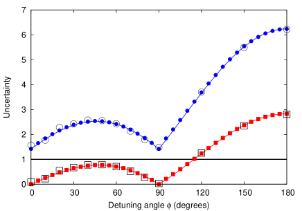
Figure 5: Uncertainties $\epsilon(A)\eta(B)+\epsilon(A)\sigma(B)+\sigma(A)\eta(B)$ (circles) and $\epsilon(A)\eta(B)$ (squares) as obtained from the event-by-event simulations (solid symbols) of the single-neutron experiment (Erhart et al., 2012; Sulyok et al., 2013), the experiment itself ((open symbols), data kindly provided to us by G. Sulyok and Y. Hasagawa) and quantum theory. The solid horizontal line represents the lowerbound in Eq. (24). The other solid lines represent the corresponding quantum theoretical prediction as obtained from Eq. (35). It is clear that the naive application of the Heisenberg uncertainty relation, $\epsilon(A)\eta(B)\geq 1$ is at odds with the prediction of quantum theory, the event-based simulation data and with the experimental data (Erhart et al., 2012; Sulyok et al., 2013). On the other hand, the experimental data (open symbols,  (Erhart et al., 2012; Sulyok et al., 2013)) and the results of the event-based simulation (solid symbols) comply with inequality Eq. (24). Left: Simulation performed using the probabilistic model for the spin analyzer, see Eq. (18). Right: Simulation performed using the deterministic learning machine model for the spin analyzer, see Eq. (19), with $\gamma=0.999$. In both cases, the number of input events per detuning angle is $N=10000$.

As shown in (Erhart et al., 2012; Sulyok et al., 2013), the neutron counts observed in the single-neutron experiment yield numerical values of $\epsilon(A)\eta(B)+\epsilon(A)\sigma(B)+\sigma(A)\eta(B)$ which are in excellent agreement with the quantum theoretical prediction $2\sqrt{2}\cos\phi\sin(\phi/2)+2\sin(\phi/2)+\sqrt{2}\cos\phi$.

We have already demonstrated that the “classical” event-based simulation model produces results for the averages which, within the statistical errors, cannot be distinguished from those predicted by quantum theory. Therefore, it is to be expected that the data generated by the event-by-event simulation also satisfies the universally valid error-disturbance uncertainty relation Eq. (24) and as shown in Fig. 5, this is indeed the case. As expected, the data produced by the event-based simulation also violate Eq. (34), independent of whether we use pseudo-random numbers (see Eq. (18)) or the DLM rule (see Eq. (19)) to model the operation of the spin analyzer.

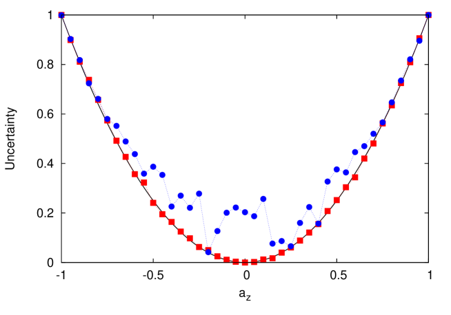
Figure 6: Event-based simulation results for $(1-\langle\sigma_{x}\rangle^{2})(1-\langle\sigma_{y}\rangle^{2})$ (blue circles) and $\langle\sigma^{z}\rangle^{2}$ (red squares) for different values of $-1\leq a_{z}\leq 1$. The solid black line represents the quantum theoretical lowerbound $a_{z}^{2}$. For each value of $a_{z}$, the initial direction of the magnetic moments is $(a_{x},a_{y},a_{z})$ where $(a_{x},a_{y})$ is a point on the circle with radius $\sqrt{1-a_{z}^{2}}$ chosen using a uniform pseudo-random number. The fluctuations of the data $(1-\langle\sigma_{x}\rangle^{2})(1-\langle\sigma_{y}\rangle^{2})$ reflect the fact that the initial states with different values of $a_{z}$ are uncorrelated. For each value of $a_{z}$, $N=10000$ messengers were created. The dotted line is a guide to the eyes only.

Finally, for the sake of completeness, we show that the event-by-event simulation produces data which complies with the standard Heisenberg-Robertson uncertainty relation $\Delta(\sigma_{x})\Delta(\sigma_{y})\geq|\langle\sigma_{z}\rangle|$. Without loss of generality, the state of the spin-1/2 particle may be represented by the density matrix Eq. (7), also if it is interacting with other degrees of freedom and the inequality $\Delta(\sigma_{x})\Delta(\sigma_{y})\geq|\langle\sigma_{z}\rangle|$ reads

$$(1-\langle\sigma_{x}\rangle^{2})(1-\langle\sigma_{y}\rangle^{2}) \geq \langle\sigma_{z}\rangle^{2},$$ (40)

or, using Eq. (7),

$$(1-a_{x}^{2})(1-a_{y}^{2}) \geq a_{z}^{2}.$$ (41)

The last inequality also trivially follows from the constraint $a_{x}^{2}+a_{y}^{2}+a_{z}^{2}\leq 1$. As in the case of Eq. (36), there is no $\hbar$ in Eq. (40), in agreement with the idea that $\hbar$ may be eliminated by re-defining the units of mass, time, etc. (Volovik, 2010; Ralston, 2013).

The simulation procedure that we use is as follows.

1. Loop over the values $(\mathbf{m}_{\mathrm{initial}})_{z}=a_{z}=-1,\ldots 1$ in small steps, e.g. in steps of 0.05.

2. Generate a uniform pseudo-random number $0<r<1$. Compute $(\mathbf{m}_{\mathrm{initial}})_{x}=a_{x}=\sqrt{1-a_{z}^{2}}\cos(2\pi r)$ and $(\mathbf{m}_{\mathrm{initial}})_{y}=a_{y}=\sqrt{1-a_{z}^{2}}\sin(2\pi r)$. This step yields a direction of the magnetization $\mathbf{m}_{\mathrm{initial}}$ which is chosen randomly in the $x-y$ plane.

3. Generate $N$ messengers with message $\mathbf{m}_{\mathrm{initial}}$ and send them through a spin analyzer aligned along the $x$-direction. Count the messengers that pass the spin analyzer. Repeat this procedure for spin analyzers aligned along the $-x$, $\pm y$ and $\pm z$-direction. Processing the $N$ messengers yields the counts $N(\mathbf{x}|\mathbf{a})$, $N(\mathbf{-x}|\mathbf{a})$, etc.

4. Compute the averages $\langle\sigma_{x}\rangle\approx(N(\mathbf{x}|\mathbf{a})-N(\mathbf{-x}|\mathbf{a}))/(N(\mathbf{x}|\mathbf{a})+N(\mathbf{-x}|\mathbf{a}))$, etc.

5. Go to step 1. as long as $a_{z}\leq 1$.

6. Plot the results for $(1-\langle\sigma_{x}\rangle^{2})(1-\langle\sigma_{y}\rangle^{2})$ and $\langle\sigma^{z}\rangle^{2}$ as a function of $a_{z}$.

The results of the event-based simulation are shown in Fig. 6. Within the usual statistical errors, the classical, statistical model produces data which comply with the Heisenberg-Robertson uncertainty relation Eq. (40).

VI Discussion

We have shown that a genuine classical event-based model can produce events such that their statistics satisfies the (generalized) Heisenberg-Robertson uncertainty relation which, according to present teaching, is a manifestation of truly quantum mechanical behavior.

One might be tempted to argue that in the event-based model, the direction of magnetic moment is known exactly and can therefore not be subject to uncertainty. However, this argument is incorrect in that it ignores the fact that the model of the spin analyzers generates (through the use of pseudo-random numbers, see Eq. (18) or the update rule Eq. (19)) a distribution of outcome frequencies. In fact, as is well-known, the variance of any statistical experiment (including those that are interpreted in terms of quantum theory) satisfies the Cramér-Rao bound, a lower bound on the variance of estimators of a parameter of the probability distribution in terms of the Fisher information (Van Trees, 1968). The Cramér-Rao bound contains, as a special case, Robertson’s inequality $\Delta(x)\Delta(p)\geq\hbar/2$ (Stam, 1959; Frieden, 1989, 2004; Kapsa et al., 2010; Kapsa and Skála, 2011; Skála et al., 2011). The observation that a classical statistical model produces data that complies with “quantum theoretical” uncertainty relations is a manifestation of this general mathematical result. The uncertainty relations provide bounds on the statistical uncertainties in the data and, as shown by our event-based simulation of the neutron experiment (Erhart et al., 2012; Sulyok et al., 2013), are not necessarily a signature of quantum physics, conjugate variables, etc.

As mentioned in the introduction, the event-based approach has successfully been applied to a large variety of single-photon and single-neutron experiments that involve interference and entanglement. In the present paper, we have shown that, without any modification, the same simulation approach can also mimic, event-by-event, an experiment that probes “quantum uncertainty”. As none of these demonstrations rely on concepts of quantum theory and as it is unlikely that the success of all these demonstrations is accidental, one may wonder what it is that makes a system genuine “quantum”.

In essence, in our work we adopt Bohr’s point of view that “There is no quantum world. There is only an abstract physical description” (reported by (Petersen, 1963), for a discussion see (Plotnitsky, 2010)) and that “The physical content of quantum mechanics is exhausted by its power to formulate statistical laws” (Bohr, 1999). Or, to say it differently, quantum theory describes our knowledge of the atomic phenomena rather than the atomic phenomena themselves (Laurikainen, 1997). In other words, our viewpoint is that quantum theory captures, and does so extremely well, the inferences that we, humans, make on the basis of experimental data (De Raedt et al., 2013). However it does not describe cause-and-effect processes. Quantum theory predicts the probabilities that events occur, but it cannot answer the question “Why are there events?” (B-G. Englert, 2013), very much as Euclidean geometry cannot answer the question “What is a point?”. On a basic level, it is our perceptual and cognitive system that defines, registers and processes events. Events and the rules that create new events are the key elements of the event-based approach. There is no underlying theory that is supposed to give rise to events and everything follows by inference on the basis of the generated data, very much like in real experiments.

The implication of the work presented in our paper is that the beautiful single-neutron experiments (Erhart et al., 2012; Sulyok et al., 2013) can be explained in terms of cause-and-effect processes in an event-by-event manner, without reference to quantum theory and on a level of detail about which quantum theory has nothing to say. Furthermore, our work suggests that the relevance of “quantum theoretical” uncertainty relations to real experiments needs to be reconsidered.

Disclosure/Conflict-of-Interest Statement

The authors declare that the research was conducted in the absence of any commercial or financial relationships that could be construed as a potential conflict of interest.

References

- Ballentine (1970) L. E. Ballentine, “The Statistical Interpretation of Quantum Mechanics,” Rev. Mod. Phys. 42, 358 – 381 (1970).
- Home (1997) D. Home, Conceptual Foundations of Quantum Physics (Plenum Press, New York, 1997).
- Ballentine (2003) L. E. Ballentine, Quantum Mechanics: A Modern Development (World Scientific, Singapore, 2003).
- Allahverdyan et al. (2013) A. E. Allahverdyan, R. Balian, and Th. M. Nieuwenhuizen, “Understanding quantum measurement from the solution of dynamical models,” Phys. Rep. 525, 1 – 166 (2013).
- Tonomura (1998) A. Tonomura, The Quantum World Unveiled by Electron Waves (World Scientific, Singapore, 1998).
- Rauch and Werner (2000) H. Rauch and S. A. Werner, Neutron Interferometry: Lessons in Experimental Quantum Mechanics (Clarendon, London, 2000).
- Garrison and Chiao (2008) J. C. Garrison and R. Y. Chiao, Quantum Optics (Oxford University Press, Oxford, 2008).
- Bohr (1999) N. Bohr, “XV. The Unity of Human Knowledge,” in Complementarity Beyond Physics (1928 –1962), Niels Bohr Collected Works, Vol. 10, edited by David Favrholdt (Elsevier, Amsterdam, 1999) pp. 155 – 160.
- Michielsen et al. (2011) K. Michielsen, F. Jin, and H. De Raedt, “Event-based corpuscular model for quantum optics experiments,” J. Comp. Theor. Nanosci. 8, 1052 – 1080 (2011).
- De Raedt and Michielsen (2012) H. De Raedt and K. Michielsen, “Event-by-event simulation of quantum phenomena,” Ann. Phys. (Berlin) 524, 393 – 410 (2012).
- De Raedt et al. (2012a) H. De Raedt, F. Jin, and K. Michielsen, “Event-based simulation of neutron interferometry experiments,” Quantum Matter 1, 1 – 21 (2012a).
- Zhao and De Raedt (2008) S. Zhao and H. De Raedt, “Event-by-event simulation of quantum cryptography protocols,” J. Comp. Theor. Nanosci. 5, 490 – 504 (2008).
- Michielsen et al. (2005) K. Michielsen, K. De Raedt, and H. De Raedt, “Simulation of quantum computation: a deterministic event-based approach,” J. Comput. Theor. Nanosci. 2, 227 – 239 (2005).
- Erhart et al. (2012) J. Erhart, S. Sponar, G. Sulyok, G. Badurek, M. Ozawa, and Y. Hasegawa, “Experimental demonstration of a universally valid error-distrurbance uncertainty relation in spin measurements,” Nat. Phys. 8, 185 – 189 (2012).
- Sulyok et al. (2013) G. Sulyok, S. Sponar, J. Erhart, G. Badurek, M. Ozawa, and Y. Hasegawa, “Violation of Heisenberg’s error-disturbance uncertainty relation in neutron-spin measurements,” Phys. Rev. A 88, 022110 (2013).
- Frieden (1989) B. R. Frieden, “Fisher information as the basis for the Schrödinger wave equation,” Am. J. Phys. 57, 1004 – 1008 (1989).
- Reginatto (1998) M. Reginatto, “Derivation of the equations of nonrelativistic quantum mechanics using the principle of minimum Fisher information,” Phys. Rev. A 58, 1775 – 1778 (1998).
- Hall (2000) M. J. W. Hall, “Quantum properties of classical Fisher information,” Phys. Rev. A 62, 012107 (2000).
- Frieden (2004) B. R. Frieden, Science from Fisher information: A unification (Cambridge University Press, Cambridge, 2004).
- Khrennikov (2009) A. Yu. Khrennikov, Contextual Approach to Quantum Formalism (Springer, Berlin, 2009).
- Khrennikov (2011) A. Yu. Khrennikov, “On the role of probabilistic models in quantum physics: Bell’s inequality and probabilistic incompatibility,” J. Comp. Theor. Nanosci. 8, 1006 – 1010 (2011).
- Khrennikov et al. (2011) A. Yu. Khrennikov, B. Nilsson, and S. Nordebo, “Classical signal model reproducing quantum probabilities for single and coincidence detections,” J. Phys.: Conf. Ser. 361, 012030 (2011).
- Kapsa et al. (2010) V. Kapsa, L. Skála, and J. Chen, “From probabilities to mathematical structure of quantum mechanics,” Physica E 42, 293 – 297 (2010).
- Skála et al. (2011) L. Skála, J. Ĉízêk, and V. Kapsar, “Quantum Mechanics as applied mathematical statistics,” Ann. Phys. 326, 1174 – 1188 (2011).
- Kapsa and Skála (2011) V. Kapsa and L. Skála, “Quantum Mechanics, Probabilities and Mathematical Statistics,” J. Comput. Theor. Nanosci. 8, 998 – 1005 (2011).
- Klein (2012) U. Klein, “What is the limit of quantum theory ?” Am. J. Phys. 80, 1009 – 1016 (2012).
- Klein (2010) U. Klein, “The statistical origins of quantum mechanics,” Physics Research International 2010, 808424 (2010).
- Flego et al. (2012) S. P. Flego, A. Plastino, and A. R. Plastino, “Fisher information and quantum mechanics,” Int. Res. J. Quant. Pure & Appl. Chem. 2, 25 – 54 (2012).
- Ozawa (2003) Masanao Ozawa, “Universally valid reformulation of the Heisenberg uncertainty principle on noise and disturbance in measurement,” Phys. Rev. A 67, 042105 (2003).
- De Raedt et al. (2011) H. De Raedt, K. Hess, and K. Michielsen, “Extended Boole-Bell inequalities applicable to quantum theory,” J. Comp. Theor. Nanosci. 8, 1011 – 1039 (2011).
- Kroupa et al. (2000) G. Kroupa, G. Bruckner, O. Bolik, M. Zawisky, M. Hainbuchner, G. Badurek, R. J. Buchelt, A. Schricker, and H. Rauch, “Basic features of the upgraded S18 neutron interferometer set-up at ILL,” Nucl. Instrum. Methods Phys. Res. A. 440, 604 – 608 (2000).
- Fujikawa (2012) Kazuo Fujikawa, “Universally valid Heisenberg uncertainty relation,” Phys. Rev. A 85, 062117 (2012).
- Leggett (1987) A. J. Leggett, “Quantum mechanics at the macroscopic level,” in The Lessons of Quantum Theory: Niels Bohr Centenary Symposium, edited by J. de Boer, E. Dal, and O. Ulfbeck (Elsevier, Amsterdam, 1987) pp. 35 – 58.
- Fujikawa and Umetsu (2013) K. Fujikawa and K. Umetsu, “Aspects of universally valid Heisenberg uncertainty relation,” Prog. Theor. Exp. Phys. 2013, 013A03 (2013).
- Robertson (1929) H. P. Robertson, “The uncertainty principle,” Phys. Rev. 34, 163–164 (1929).
- Heisenberg (1927) W. Heisenberg, “Über den anschaulichen Inhalt der quantentheoretischen Kinematik and Mechanik,” Z. Phys. 43, 172–198 (1927).
- Busch et al. (2007) Paul Busch, Teiko Heinonen, and Pekka Lahti, “Heisenberg’s uncertainty principle,” Physics Reports 452, 155 – 176 (2007).
- Busch et al. (2013) Paul Busch, Pekka Lahti, and Reinhard F. Werner, “Proof of Heisenberg’s error-disturbance relation,” Phys. Rev. Lett. 111, 160405 (2013).
- Van Trees (1968) H. L. Van Trees, Detection, Estimation, and Modulation Theory (Part I) (John Wiley, New York, 1968).
- Boole (1862) G. Boole, “On the theory of probabilities,” Phil. Trans. R. Soc. Lond. 152, 225 – 252 (1862).
- Volovik (2010) G.E. Volovik, “ as parameter of Minkowski metric in effective theory ,” JETP Lett. 90, 697 – 704 (2010).
- Ralston (2013) J. P. Ralston, “Revising your world-view of the fundamental constants,” Proc. SPIE 8832, 883216–1 – 883216–16 (2013).
- Vorob’ev (1962) N. N. Vorob’ev, “Consistent families of measures and their extensions,” Theor. Probab. Appl. 7, 147 – 162 (1962).
- Ballentine (1986) L. E. Ballentine, “Probability-theory in quantum-mechanics,” Am. J. Phys. 54, 883 – 889 (1986).
- Sinha et al. (2010) U. Sinha, C. Couteau, T. Jennewein, R. Laflamme, and G.Weihs, “Ruling out multi-order interference in quantum mechanics,” Science 329, 418 – 421 (2010).
- De Raedt et al. (2012b) H. De Raedt, K. Michielsen, and K. Hess, “Analysis of multipath interference in three-slit experiments,” Phys. Rev. A 85, 012101 (2012b).
- Fine (1982) A. Fine, “Hidden variables, joint probability, and Bell inequalities,” Phys. Rev. Lett. 48, 291 – 295 (1982).
- Hess and Philipp (2001) K. Hess and W. Philipp, “A possible loophole in the theorem of Bell,” Proc. Natl. Acad. Sci. USA 98, 14224 – 14277 (2001).
- Stam (1959) A. J. Stam, “Some inequalities satisfied by the quantities of information of Fisher and Shannon,” Information and Control 2, 101 – 112 (1959).
- Petersen (1963) A. Petersen, “The philosophy of Niels Bohr,” Bull. Atomic Scientists 19, 8 – 14 (1963).
- Plotnitsky (2010) A. Plotnitsky, ”Epistemology and Probability: Bohr, Heisenberg, Schrödinger, and the Nature of Quantum-Theoretical Thinking” (Springer, Berlin, 2010).
- Laurikainen (1997) K. V. Laurikainen, The Message of the Atoms. Essays on Wolfgang Pauli and the Unspeakable (Springer, Berlin, 1997).
- De Raedt et al. (2013) H. De Raedt, M.I. Katsnelson, and K. Michielsen, “Quantum theory as the most robust description of reproducible experiments,” (2013), arXiv/quant-ph/1303.4574.
- B-G. Englert (2013) B-G. Englert, “On quantum theory,” Eur. Phys. J. D 67, 238 (2013).