Gravitational wave momentum extraction in non-axisymmetric Robinson-Trautman spacetimes

Abstract

We examine numerically the gravitational wave recoil in non-axisymmetric Robinson-Trautman spacetimes. We construct characteristic initial data for the Robinson-Trautman dynamics which are interpreted as corresponding to the early post-merger state of two boosted colliding black holes with a common apparent horizon. Our analysis is based on the Bondi-Sachs energy-momentum conservation laws which regulate the radiative transfer processes involved in the emission of gravitational waves. We evaluate the Bondi-Sachs momentum flux carried out by gravitational waves and the associated net kick velocity defined (in a zero-initial-Bondi-momentum frame) as proportional to the total gravitational wave impulse imparted on the system. The kick velocity distributions are obtained and analyzed for two distinct classes of initial data corresponding to the early post-merger state of (i) non-head-on collisions and (ii) head-on collisions of black holes. For the first class (i), the net gravitational wave momentum fluxes and associated kicks are evaluated for a given domain of parameters (incidence angle and mass ratio). Typically for the equal mass case the net gravitational wave momentum flux carried is nonzero. This last result indicates that these configurations are not connected with black hole binary inspirals or head-on collisions. We suggest that these systems might be a candidate to an approximate description of the post-merger phase of a non-head-on collision of black holes not preceded by a pre-merger inspiral phase, as for instance colliding black holes in pre-merger unbounded trajectories. For the second class (ii), head-on collisions, we compare our results, and discuss the analogies, with $1+3$ numerical relativity simulations of binary black hole inspirals and head-on collisions.

I Introduction

The collision and merger of two black holes is presently considered to be an important astrophysical configuration where processes of generation and emission of gravitational waves take place (cf. [1] and references therein). The radiative transfer involved in these processes, evaluated in the full nonlinear regime of General Relativity, shows that gravitational waves extract mass, momentum and angular momentum of the source, and may turn out to be fundamental for the astrophysics of the collapse of stars and the formation of black holes. The process of momentum extraction and the associated recoils in the system can have important consequences for astrophysical scenarios, as the evolution and the population of massive black holes in galaxies or in the intergalactic medium[2, 3, 4]. Observational evidence of black hole recoils have been reported in [5] and references therein.

The kick processes and associated recoils in the merger of two black holes have been investigated within several approaches, most of them connected to binary black hole inspirals. Post-Newtonian approximations (cf. [6] and references therein) estimated the kick velocity accumulated during the adiabatical inspiral of the system plus the kick velocity accumulated during the plunge phase. Sopuerta et al.[7] computed the recoil velocity based on the close limit approximation (CLA) supplemented with post-Newtonian (PN) calculations, and estimated a lower bound for the kick velocity in binaries with a mass ratio $\simeq 0.34$. The first full numerical relativity evaluation of the recoil in nonspinning black hole binaries was reported by Baker et al.[2] for a mass ratio $\simeq 0.667$ of the two black holes, while González et al.[8] and Campanelli et al.[9] simultaneously obtained much larger recoils for black hole binaries with antialigned spins. González et al.[10] undertook a more complete full numerical relativity examination of kicks in the merger of nonspinning black hole binaries by contemplating a larger parameter domain. For the case of small mass ratios in the interval $0.01\leq\alpha\leq 0.1$ full numerical relativity evaluations bridged with perturbative techniques were implemented in Refs. [11, 12, 13, 14]. Le Tiec et al.[15], combining PN+CLA methods, recently evaluated the gravitational wave recoil in black hole binaries and showed that the ringdown (evaluated within the CLA) produces a significant anti-kick. In the same vein Choi et al.[16] examined recoils in head-on collisions of spinning and nonspinning black holes, considering the head-on case as a model problem which can be seen as an approximation to the final plunge to merger and allow to isolate kick effects from the orbital inspiral motion. Finally Rezzola et al.[17, 18] obtained an important injective relation between the kick velocities and the effective curvature parameter of the global apparent horizon, in head-on collisions, using initial data derived in [19, 20].

From numerical relativity $3+1$ evaluations we have evidence that an important contribution to the gravitational wave recoil comes from the post-merger phase, where also a final deceleration regime is present leading to the so termed anti-kicks in the system. In the present paper we intend to approach some of these issues by examining the gravitational wave recoil in non-axisymmetric Robinson-Trautman (RT) spacetimes[21] in the Bondi-Sachs (BS) characteristic formulation of gravitational wave emission[22, 23]. The paper extends and completes Ref. [24] where we examined numerically the gravitational wave production and related radiative processes using initial data that are interpreted as describing the post-merger phase of non-head-on colliding black holes. Our numerical codes are accurate and sufficiently stable for long time runs so that we are able to reach numerically the final configuration of the system, when the gravitational emission ceases. RT spacetimes already present an apparent horizon so that the dynamics covers the post merger phase of the system up to the final configuration of the remnant black hole. Due to the presence of a global apparent horizon the initial data effectively represents an initial single distorted black hole which is evolved via the RT dynamics. Similarly to the case of the CLA – where the perturbation equations of a black hole[25, 26] are feeded either with numerically generated, or with Misner, or Bowen-York-type initial data – we feed the (nonlinear) RT equation with the above mentioned characteristic data. It is in this sense that we denote the dynamics thus generated as “the post-merger phase of two colliding black holes”. The interpretation of the outcomes of the RT dynamics and its comparison, in the head-on case, with numerical relativity results should be considered with the above caveats.

RT spacetimes[21] are asymptotically flat solutions of Einstein’s vacuum equations that describe the exterior gravitational field of a bounded system radiating gravitational waves. In a suitable coordinate system the metric can be expressed as

$$ds^{2} = \Big{(}{\lambda(u,\theta,\phi)-\frac{2m_{0}}{r}+2r\frac{{K}_{,u}}{K}}\Big{)}du^{2}+2dudr$$ (1)

$$- r^{2}K^{2}(u,\theta,\phi)~{}\Big{(}d\theta^{2}+\sin^{2}\theta d\phi^{2}\Big{)},$$

where

$$\lambda(u,\theta,\phi)=\frac{1}{K^{2}}-\frac{(K_{,\theta}~{}\sin\theta/K)_{,\theta}}{K^{2}\sin\theta}+\frac{1}{\sin^{2}\theta}\Big{(}\frac{K_{,\phi}^{2}}{K^{4}}-\frac{K_{,\phi\phi}}{K^{3}}\Big{)}.$$ (2)

The Einstein vacuum equations for (1) result in

$$-6m_{0}\frac{{K}_{,u}}{K}+\frac{1}{2K^{2}}\Big{(}\frac{(\lambda_{,\theta}\sin\theta)_{,\theta}}{\sin\theta}+\frac{\lambda_{,\phi\phi}}{\sin^{2}\theta}\Big{)}=0.$$ (3)

Subscripts $u$, $\theta$ and $\phi$, preceded by a comma, denote derivatives with respect to $u$, $\theta$ and $\phi$, respectively. $m_{0}>0$ is the only dimensional parameter of the geometry, which fixes the mass and length scales of the spacetime. Eq. (3), the RT equation, governs the dynamics of the system and allows to evolve the initial data $K(u_{0},\theta,\phi)$, given in the characteristic surface $u=u_{0}$, for times $u>u_{0}$. For sufficiently regular initial data RT spacetimes exist globally for all positive $u$ and converge asymptotically to the Schwarzschild metric as $u\rightarrow\infty$[27]. Once the initial data $K(u_{0},\theta,\phi)$ is specified, a unique apparent horizon (AH) solution is fixed for that $u_{0}$[28]. Since the AH is the outer past marginally trapped surface, the closest of a white hole definition (the remnant black hole will form as $u\rightarrow\infty$), only the exterior and its future development via RT dynamics with outgoing gravitational waves is of interest. We note that all the BS quantities, measured at the future null infinity $\mathcal{J}^{+}$, are constructed and well defined under the outgoing radiation condition[17,18].

The field equations have a stationary solution which will play an important role in our discussions,

$$K(\theta,\phi)=\frac{K_{0}}{\cosh\gamma+({\bf{n}}\cdot\hat{\bf{x}})\sinh\gamma},$$ (4)

where $\hat{\bf{x}}=(\sin\theta\cos\phi,\sin\theta\sin\phi,\cos\theta)$ is the unit vector along an arbitrary direction ${\bf{x}}$, and ${\bf{n}}=(n_{1},n_{2},n_{3})$ is a constant unit vector satisfying $n_{1}^{2}+n_{2}^{2}+n_{3}^{2}=1$. The $K_{0}$ and $\gamma$ are constants. We note that (4) yields $\lambda=1/K_{0}^{2}$, resulting in its stationary character (cf. eq. (3)). This solution can be interpreted[22] as a boosted Schwarzschild black hole along the axis determined by ${\bf{n}}$, with boost parameter $\gamma$ (or velocity parameter $v=\tanh\gamma$). For $\gamma=0$ we recover the Schwarzschild black hole at rest.

The Bondi mass function of (4) is $m(\theta,\phi)=m_{0}K^{3}(\theta,\phi)$, and the total mass-energy of this gravitational configuration is given by the Bondi mass

$$M_{B} = \frac{1}{4\pi}\int^{2\pi}_{0}d\phi\int^{\pi}_{0}m(\theta,\phi)\sin\theta~{}d\theta$$ (5)

$$= m_{0}K_{0}^{3}\cosh\gamma=m_{0}K_{0}^{3}/\sqrt{1-v^{2}}.$$

The interpretation of (4) as a boosted black hole is relative to the asymptotic Lorentz frame which is the rest frame of the black hole when $\gamma=0$.

In the paper we use geometrical units $G=c=1$; $c$ is however restored in the definition of the kick velocity. Except where explicitly stated, all the numerical results are for $\gamma=0.5$ fixed. In our computations we adopted $m_{0}=10$ but the results are given in terms of $u/m_{0}$. We note that we can always set $m_{0}=1$ in RT equation (3) by the transformation $u\rightarrow{\tilde{u}}=u/m_{0}$.

II The Bondi-Sachs four momentum for RT spacetimes, the news and the initial data

Since RT spacetimes describe asymptotically flat radiating spacetimes and the initial data for the dynamics are prescribed on null characteristic surfaces, they are in the realm of the $2+2$ Bondi-Sachs (BS) formulation of gravitational waves in General Relativity[22, 23, 29]. Therefore we shall use the physical quantities of this formulation which appear in the description of gravitational wave emission processes, as the BS four-momentum and its conservation laws. A detailed derivation of the BS four-momentum conservation laws in RT spacetimes was given in [30] but, for the sake of clarity, a few fundamental results are discussed in the following. From the supplementary vacuum Einstein equations $R_{UU}=0$, $R_{U\Theta}=0$, and $R_{U\Phi}=0$ in the BS formulation (where $(U,R,\Theta,\Phi)$ are Bondi-Sachs coordinates), we obtain[22, 23]

$$\frac{\partial m(u,\theta,\phi)}{\partial u}=-K\Big{(}{c_{,u}^{(1)}}^{2}+{c_{,u}^{(2)}}^{2}\Big{)}+\frac{1}{2}\frac{\partial}{\partial u}\Big{[}3c_{,\theta}^{(1)}\cot\theta$$ (6)

$$+ 4c_{,\phi}^{(2)}\frac{\cos\theta}{\sin^{2}\theta}-2c^{(1)}+c_{,\theta\theta}^{(1)}+\frac{2}{\sin\theta}c_{,\theta\phi}^{(2)}-\frac{1}{\sin^{2}\theta}c_{,\phi\phi}^{(1)}\Big{]},$$

where $m(u,\theta,\phi)$ is the Bondi mass function and $c_{,u}^{(1)}(u,\theta,\phi)$ and $c_{,u}^{(2)}(u,\theta,\phi)$ are the two news functions, in RT coordinates. The extra factor $K$ in the first term of the right-hand-side of Eq. (6) comes from the transformation of the Bondi time coordinate $U$ to the RT coordinate $u$, ${\rm lim}_{r\rightarrow\infty}=\partial U/\partial u=1/K$. For the RT spacetimes (1), the news are expressed as[30]

$$c_{,u}^{(1)}(u,\theta,\phi) = \frac{1}{2}\Big{(}{\mathcal{P}}_{,\theta\theta}-{\mathcal{P}}_{,\theta}\cot\theta-\frac{{\mathcal{P}}_{,\phi\phi}}{\sin^{2}\theta}\Big{)},$$

$$c_{,u}^{(2)}(u,\theta,\phi) = \frac{1}{\sin\theta}\Big{(}{\mathcal{P}}_{,\theta\phi}-{\mathcal{P}}_{,\phi}\cot\theta\Big{)},$$ (7)

where we have introduced the variable ${\mathcal{P}}\equiv 1/K$, for notation convenience. We remark that $c^{(1)}_{,u}=0=c^{(2)}_{,u}$ for the boosted Schwarzschild solution (4), as should be expected.

The Bondi-Sachs four momentum is defined as[29]

$$P^{\mu}(u)=\frac{1}{4\pi}\int^{2\pi}_{0}d\phi\int^{\pi}_{0}m(u,\theta,\phi)~{}l^{\mu}\sin\theta~{}d\theta,$$ (8)

where $l^{\mu}=(1,-\sin\theta\cos\phi,-\sin\theta\sin\phi,-\cos\theta)$, relative to an asymptotic Lorentz frame. From Eq. (6) the Bondi-Sachs four momentum conservation law follows

$$\frac{dP^{\mu}(u)}{du}=P_{W}^{\mu}(u),$$ (9)

where

$$P_{W}^{\mu}(u)=-\frac{1}{4\pi}\int^{2\pi}_{0}d\phi\int^{\pi}_{0}K~{}l^{\mu}\Big{(}{c_{,u}^{(1)}}^{2}+{c_{,u}^{(2)}}^{2}\Big{)}\sin\theta~{}d\theta~{}~{}$$ (10)

is the net flux of energy-momentum carried out by the the gravitational waves emitted. We note that the term between square brackets in the right-hand-side of (6) vanishes in the integrations due to the boundary conditions satisfied by the news, $c^{(1)}=c^{(2)}=0$ and $c^{(1)}_{\theta}=c^{(2)}_{\theta}=0$ at $\theta=0,\pi$. The mass-energy conservation law (Eq. (9) for $\mu=0$) is the Bondi mass formula. Our main interest here is the analysis of the linear momentum conservation, Eq. (9) for $\mu=x,y,z$,

$$\frac{d{\bf P}(u)}{du}={\bf P}_{W}(u),$$ (11)

where ${\bf P}_{W}(u)=(P^{x}_{W}(u),P^{y}_{W}(u),P^{z}_{W}(u))$, with

$${P}_{W}^{x}(u) = \frac{1}{4\pi}\int^{2\pi}_{0}d\phi\int^{\pi}_{0}\sin^{2}\theta\cos\phi~{}K\Big{(}{c_{,u}^{(1)}}^{2}+{c_{,u}^{(2)}}^{2}\Big{)}d\theta,~{}~{}~{}~{}~{}~{}$$ (12)

$${P}_{W}^{y}(u) = \frac{1}{4\pi}\int^{2\pi}_{0}d\phi\int^{\pi}_{0}\sin^{2}\theta\sin\phi~{}K\Big{(}{c_{,u}^{(1)}}^{2}+{c_{,u}^{(2)}}^{2}\Big{)}d\theta,~{}~{}~{}~{}$$ (13)

$${P}_{W}^{z}(u) = \frac{1}{4\pi}\int^{2\pi}_{0}d\phi\int^{\pi}_{0}\cos\theta\sin\theta~{}K\Big{(}{c_{,u}^{(1)}}^{2}+{c_{,u}^{(2)}}^{2}\Big{)}d\theta.~{}~{}~{}~{}$$ (14)

Figure 1: Schematic diagram illustrating the initial data (15) corresponding to the non-head-on collision of two black holes, reproduced from [24]. The dashed line depicts the common apparent horizon (AH). The remnant black hole is also displayed, where $\rho_{f}$ defines its direction of motion. The $x$-axis is upward.

The characteristic initial data to be used was derived in [24] and can be interpreted as describing the early post-merger configuration of two colliding black holes in the $(x,z)$ plane, at $u=u_{0}$,

$$K(u_{0},\theta,\phi)=\Big{(}\frac{\alpha_{1}}{\sqrt{{\cosh\gamma+\cos\theta\sinh\gamma}}}+$$

$$\frac{\alpha_{2}}{\sqrt{{\cosh\gamma-(\cos\rho_{0}~{}\cos\theta-\sin\rho_{0}~{}\sin\theta\cos\phi)\sinh\gamma}}}\Big{)}^{2}.~{}~{}~{}~{}~{}$$ (15)

In the derivation of (15) it turns out that $\alpha_{2}/\alpha_{1}$ is the mass ratio of the Schwarzschild masses of the initial data, as seen by an asymptotic observer. We also mention the following properties of (15): (i) for $\alpha_{2}=0$ ($\alpha_{1}\neq 0$) or $\alpha_{1}=0$ ($\alpha_{2}\neq 0$) the initial data (15) corresponds to a boosted Schwarzschild black hole along, respectively, the positive $z$-axis or along the direction of the unit vector ${\bf n}=(-\cos\rho_{0},0,\sin\rho_{0})$, with respect to an asymptotic Lorentz frame (cf. eq. (4)). (ii) The specific combination (15) of two boosted black hole solutions (4) is not arbitrary but arises as the conformal factor of an asymptotically flat 3-geometry which is a solution of the constraint ${}^{(3)}R=0$. (iii) Additionally (15) results in a planar dynamics, namely, for all $u$ the net gravitational wave momentum flux ${\bf P}_{W}(u)$ is restricted to the plane determined by the unit vectors ${\bf n}_{z}$ and ${\bf n}$ defining the direction of motion of the two black holes entering in (15), namely, the $(x,z)$-plane. Therefore we have that $P_{W}^{y}(u)=0$ for all $u$, implying obviously that $P^{y}(u)$ is conserved. The momentum of the remnant is also contained in this plane, as should be expected. (iv) The data (15) with $\rho_{0}=0^{\circ}$ is the only combination of the black hole solutions (4) that results in a distribution for the recoils satisfying a Fitchett law, as shown in the many numerical tests we have performed. The above properties are consistent with the interpretation of (15) as related to the early post-merger state of a black hole collision.

As concerning the parameter $\rho_{0}$, the data corresponds to bring instantaneously in interaction the two individual boosted black holes, each described by equation (4), one along the $z$ axis (${\bf{n}}=(0,0,1)$) and the other with $\bf{n}$ making an angle $\rho_{0}$ with the $z$-axis of the asymptotic Lorentz observer. $\gamma$ is the boost parameter of the black hole solutions (4) which enter in (15). As in the characteristic and $1+3$ numerical relativity approaches, the interpretation of the initial data parameters involves an approximation, namely, that the initial gravitational interaction in the data is neglected. A schematic diagram of the initial data is given in Fig. 1, reproduced from [24]. As mentioned already this data has a common apparent horizon so that the evolution covers the post merger regime up to the final configuration, when the gravitational wave emission ceases. In the remaining of the paper we fix $\alpha_{1}=1$ and relabel $\alpha_{2}\equiv\alpha$.

Finally we must address the issue of junk radiation as concerning our initial data. In fact, on evolving the system, we did not obtain evidence of any junk radiation component present in the initial data. The time behavior of the radiated energy and momentum fluxes, from the initial configuration up to the final configuration, is very smooth, with no transient component or “bump” in its early evolution. This can be seen, for instance, in the momentum fluxes of Figs. 2 and 3(top) of Section IV, where the initial domain of the time axes is stretched by the use of a log scale. This pattern of the fluxes is stable for variations of the parameters of the initial data. Similarly the gravitational wave energy fluxes (examined in [24]) decrease monotonically with $u$ for any domain of parameters. Therefore the result of a non-zero gravitational wave recoil for $\alpha=1$ and $\rho_{0}\neq 0$ reported in Section IV is unlikely to be a contribution of a junk radiation component.

III Numerical evolution

The initial data (15) is evolved numerically via the RT equation (3), which is integrated using a Galerkin spectral method with a spherical harmonics projection basis space[31] adapted to the non-axisymmetric dynamics of RT spacetimes. The implementation of the Garlenkin method is described in detail in Section V of Ref. [24], as well as its accuracy and stability for long time runs. However for completeness we present here a brief survey of the method.

Table 1: $\chi_{1}(u)\equiv\big{(}A_{N_{P},0}/A_{0,0}\Big{)}(u)$, $\chi_{2}(u)\equiv\Big{(}A_{N_{P},N_{P}}/A_{0,0}\Big{)}(u)$, $u_{f}\simeq 460$.

	$\chi_{1}(0)$,  $\chi_{2}(0)$	$\chi_{1}(110)$,  $\chi_{2}(110)$	$\chi_{1}(250)$,  $\chi_{2}(250)$	$\chi_{1,2}(u_{f})$
$N_{P}=5$	1.0 e-4,  2.8 e-10	1.3e-6,  0	0.8 e-9,  0	$0$
$N_{P}=6$	-9.2 e-6, -1.9 e-12	-2.5 e-7, 0	-1.6 e-10, 0	$0$
$N_{P}=7$	2.0 e-6, 1.0 e-14	4.3 e-8, 0	2.7 e-11, 0	$0$

For convenience we will use the function ${\mathcal{P}}(u,\theta,\phi)\equiv 1/K(u,\theta,\phi)$. The Galerkin method establishes that ${\mathcal{P}}(u,\theta,\phi)$ can be expanded in a convenient set of basis functions of a projection space (in this case the real spherical harmonics basis) through which we can reduce the RT partial differential equation into an autonomous nonlinear dynamical system for the modal coefficients $(A_{l,m}(u),B_{l,m}(u))$ of the expansion ${\mathcal{P}}(u,\theta,\phi)=\sum_{l=1}^{N_{P}}\sum_{m=1}^{l}A_{l,m}(u)P_{l}^{m}(\cos\theta)\cos m\phi+\sum_{l=1}^{N_{P}}\sum_{m=1}^{l}B_{l,m}(u)P_{l}^{m}(\cos\theta)\sin m\phi$, where $P_{l}^{m}(\cos\theta)$ are the associated Legendre functions properly normalized. Projecting this expression on each element of the basis of the projection space (using the ${\mathcal{L}}^{2}$ norm and the orthonormal relations of the basis under this norm) we obtain the modal coefficients $A_{l,m}(u)$ , $B_{l,m}(u)$ for the corresponding ${\mathcal{P}}(u,\theta,\phi)$. $N_{P}$ is the truncation of the method and, together with the choice of the projection space, constitutes a fundamental cornerstone of the method. Substituting this expansion, and its time and angle derivatives, in the RT equation (3) and projecting on each element of the basis we obtain an autonomous dynamical system of dimension $(N_{P}+1)^{2}$ for the modal coefficients, ${\dot{A}}_{l,m}(u)={\mathcal{A}}_{l,m}\Big{(}A_{l,m}(u),B_{l,m}(u)\Big{)}$, ${\dot{B}}_{l,m}(u)={\mathcal{B}}_{l,m}\Big{(}A_{l,m}(u),B_{l,m}(u)\Big{)}$, where ${\mathcal{A}}_{l,m}$ and ${\mathcal{B}}_{l,m}$ are polynomials of order $(N_{P}+1)^{2}$ in $A_{l,m}(u)$ and $B_{l,m}(u)$. Contrary to usual numerical methods, whose objective is to obtain an approximate solution of the exact dynamics, the Galerkin method in essence has the task of obtaining the solution of an approximate dynamics described by the above dynamical system. The approximation consists in choosing a suitable finite $N_{P}$ that makes the method sufficiently accurate and saves computational effort. Of course the exact dynamics corresponds to $N_{P}=\infty$. In the integration of the autonomous dynamical system for the modal coefficients we used a fourth-order Runge-Kutta recursive method (adapted to our constraints) together with a C++ integrator[24]. For the numerical calculations in this paper we adopted $N_{P}=7$, which approximates quite well not only the initial data but also the dynamics, as we discuss now. In the above paragraph the $u$-derivative was denoted by a superscript dot to avoid the overcluttering of indices in the formulas.

A basic numerical test for the accuracy of the dynamics is connected to the planar nature of the collision for initial data in which the initial directions of motion $({\bf n}_{z},{\bf n})$ are restricted to an arbitrary plane[24]. The approximated dynamics of the modal coefficients $(A_{l,m}(u),B_{l,m}(u))$ with $N_{P}=7$ preserves accurately the planar motion which has led us to the simplified form (15), corresponding to initial motion in the $x-z$ plane. In this case the modal coefficients $B_{l,m}(u)$ are zero for all $u$ (within machine precision, meaning $\leq 10^{-14}$) and a lot of computational effort is saved by reducing the Galerkin expansion to the $\cos m\phi$ series, with the dynamics restricted to the modal coefficients $A_{l,m}$ only. In this instance the Bondi-Sachs momentum in the $y$-direction must be conserved and the net momentum flux $P_{W}^{y}(u)=0$ for all $u$. This is accurately maintained by the numerical evolution of the modal coefficients $A_{l,m}(u)$ with truncation $N_{P}=7$, namely, the reconstructed net momentum flux $P_{W}^{y}(u)=0$ for all $u$, within machine precision.

Also the power in the highest modes $l=7$ is relatively very small at all times as compared to the lowest dynamical mode $A_{0,0}$, so that the convergence of the method is guaranteed. We illustrate this with the initial data for $\alpha=0.2$, $\rho_{0}=21^{\circ}$ and $\gamma=0.5$. In all our computations we adopted $m_{0}=10$. In Table 1 we give the ratio of the highest modes, $\chi_{1}(u)\equiv A_{N_{P},0}/A_{0,0}$ and $\chi_{2}(u)\equiv A_{N_{P},N_{P}}/A_{0,0}$ for truncations $N_{P}=5$, $N_{P}=6$ and $N_{P}=7$, sampled for several times from $u=0$ to the final time of computation $u=u_{f}\simeq 460$, when all modal coefficients are zero (within machine precision) except $A_{0,0}$, $A_{0,1}$ and $A_{1,1}$. These latter nonzero modal coefficients characterize the remnant black hole.

Table 2: The net kick velocity $V_{k}$ (km/s) for several values of $\alpha$ and truncations $N_{P}=5$, $N_{P}=6$ and $N_{P}=7$.

	$\alpha=0.1$	$\alpha=0.3$	$\alpha=0.5$	$\alpha=0.9$
$N_{P}=5$	25.068	97.036	120.288	108.474
$N_{P}=6$	25.231	97.298	120.430	108.448
$N_{P}=7$	25.251	97.327	120.430	108.455

The corresponding integrated error in the approximation of the initial data, $R(u_{0},\phi)=\int_{0}^{\pi}{\mathcal{R}}(u_{0},\theta,\phi)\sin\theta d\theta$ (where ${\mathcal{R}}(u_{0},\theta,\phi)=|{\mathcal{P}}(u_{0},\theta,\phi)-{\mathcal{P}}_{\rm appr}(u_{0},\theta,\phi)/{\mathcal{P}}(u_{0},\theta,\phi)|$) is $\leq 8.3\times 10^{-6}$ for $N_{P}=6$, and $\leq 1.6\times 10^{-6}$ for $N_{P}=7$ for all $\phi$. These orders of magnitude are maintained for the domain of $\alpha$ considered, and up to $\gamma=0.7$. The smaller error $\leq 6.7\times 10^{-10}$ reported in [24] is related to a boost parameter $\gamma=0.2$. The maximum relative errors ${\mathcal{R}}(u_{0},\theta,\phi)$ have orders of magnitudes $\sim 10^{-5}$ for $N_{P}=5$ and $\sim 10^{-6}$ for $N_{P}=6$ and $N_{P}=7$, but for a substantial domain of $(\theta,\phi)$ these errors can be extremely small.

The best indicator to the accuracy of the expansion of the initial data, and of the RT dynamics for a given truncation $N_{P}$, is the behavior of the constant of motion present in RT dynamics, $\zeta(u)=(1/4\pi)\int^{2\pi}_{0}d\phi\int^{\pi}_{0}K^{2}(u,\theta,\phi)\rm sin\theta d\theta$. Its exact value can be obtained using the exact initial data which, for the present case $\alpha=0.2,~{}\gamma=0.5,~{}\rho_{0}=21^{\circ}$, is $\zeta_{\rm exact}=1.94727076130606$. For the approximated initial data, with truncation $N_{P}=7$, we obtain the value $\zeta_{\rm appr}(u=0)=1.94727076160249$ with an error $\Delta\zeta(0)=|\zeta_{\rm exact}-\zeta_{\rm appr}(u=0)|\sim 2.9\times 10^{-10}$. For all $0<u\leq u_{f}$ we have a relative error $\Delta\zeta(u)/\zeta_{\rm exact}\leq 10^{-5}~{}\%$. For the sake of completeness of this section, and anticipating results of section IV, we show in Table 2 values of the net kick velocity $V_{k}$ for $\rho_{0}=21^{\circ}$, $\gamma=0.5$ and several values of $\alpha$, for truncations $N_{P}=5$, $N_{P}=6$ and $N_{P}=7$, which also indicates that the truncation $N_{P}=7$ is sufficiently accurate.

The numerical method is stable for long time runs so that we are able to reach the final configuration of the remnant black hole when the gravitational wave emission ceases[24]. We can thus examine physical phenomena in the nonlinear regime where full numerical relativity simulations might present some difficulties due, for instance, to the limited computational domain. In this sense the results of the evolution of the above data may be considered as complementary to full numerical relativity simulations on describing the post-merger regime.

Our numerical work in the present paper contemplates the whole interval $\alpha=[0,1]$ with fixed $\rho_{0}=21^{\circ}$ and $\gamma=0.5$. For comparison purposes, results for other values of $\rho_{0}$ and $\gamma$ are also considered. Exhaustive numerical experiments show that after a sufficiently long time $u\sim u_{f}$ all modal coefficients of the Galerkin expansion become constant up to twelve significant digits, corresponding to the final time of computation $u_{f}$. At $u_{f}$ the gravitational wave emission is considered to effectively cease. In fact, all the modal coefficients are zero at $u=u_{f}$ except $A_{0,0}$, $A_{0,1}$ and $A_{1,1}$. From the final constant modal coefficients we reconstruct $K(u_{f},\theta,\phi)$ that, in all cases, can be approximated as

$$K(u_{f},\theta,\phi)\simeq\frac{K_{f}}{\cosh\gamma_{f}+(n_{1f}\sin\theta\cos\phi+n_{3f}\cos\theta)\sinh\gamma_{f}},~{}~{}$$ (16)

where

$$n_{3f} = \Big{(}1+\Big{(}2A_{1,1}(u_{f})/A_{1,0}(u_{f})\Big{)}^{2}\Big{)}^{-1/2},$$

$$n_{1f} = \Big{(}2A_{1,1}(u_{f})/A_{1,0}(u_{f})\Big{)}~{}n_{3f},$$ (17)

$$\gamma_{f} = \tanh^{-1}\Big{(}A_{1,0}(u_{f})/n_{3f}A_{0,0}(u_{f})\Big{)},$$

$$K_{f} = 2\cosh\gamma_{f}/A_{0,0}(u_{f}).$$

An alternative to evaluate the parameter $K_{f}$ is the use of the initial data in the conserved quantity $\zeta(u)$. With the final parameters $(K_{f},\gamma_{f},n_{1f},n_{3f})$ obtained from the final modal coefficients, we have in all cases that the rms error of Eq. (16) is of the order of, or smaller than $10^{-12}$. The final configuration corresponds then to a boosted Schwarzschild black hole (cf. (4)) with a final velocity $v_{f}={\rm tanh}\gamma_{f}$ along the direction determined by ${\bf{n}}_{f}=(n_{1f},0,n_{3f})$, and a final Bondi rest mass $m_{0}K_{f}^{3}$. In general $\gamma_{f}<\gamma$ and $K_{f}>1$. The angle $\rho_{f}=\arccos~{}(n_{3f})$ defines the direction of the remnant with respect to the $z$-axis. Within the numerical error of our computation we have $(n_{1f})^{2}+(n_{3f})^{2}=1$, as expected.

The values of the parameters of the remnant black hole are one of the basic results to be extracted from our numerical experiments. Also, by reconstructing $K(u,\theta,\phi)$ for all $u>u_{0}$, we can obtain the time behavior of important physical quantities, as for instance the total impulse imparted to the merged system by the emission of gravitational waves. Our numerical results are displayed in Table 3 and constitute the basis of the analysis of the gravitational wave recoil, in the next Section.

IV Gravitational wave momentum fluxes and the kick processes in a non-head-on collision

We can now discuss the processes of momentum extraction of the system by constructing, via the numerically integrated function $K(u,\theta,\phi)$, the time evolution of the net momentum fluxes carried out by gravitational waves. In Fig. 2 (top) we display the curves of the net momentum fluxes $P_{W}^{x}(u)$ and $P_{W}^{z}(u)$ for mass ratios $\alpha=0.2,~{}0.5$. We see that an initial regime of positive flux $P_{W}^{z}(u)$ is present with consequent increase of the linear momentum along the $z$-axis. $P_{W}^{x}(u)$ is negative for all $u_{0}<u\leq u_{f}$. Therefore the main contribution to the associated impulses comes from the final dominant deceleration regime until the system reaches the final configuration of the remnant black hole. The initial regime of positive flux $P_{W}^{z}(u)$ is not present in the case of large $\alpha$ and $\rho_{0}$.

IV.1 The integrated fluxes of gravitational waves and the total impulse imparted to the merged system

Integrating in time the conservation Eq. (11) we find that

$${\bf P}(u)-{\bf P}(u_{0})={\bf I}_{W}(u),$$ (18)

where ${\bf I}_{W}(u)=({I}_{W}^{x}(u),0,{I}_{W}^{z}(u))$ is the impulse imparted to the merged system by the gravitational waves emitted up to the time $u$. In the above,

$${I}_{W}^{x}(u)=\int^{u}_{u_{0}}P_{W}^{x}(u)~{}du,~{}~{}~{}{I}_{W}^{z}(u)=\int^{u}_{u_{0}}P_{W}^{z}(u)~{}du,$$ (19)

cf. Eqs. (12)-(13). The net total impulse imparted to the system has a dominant contribution from the deceleration regime (when ${\bf{I}}_{W}<0$) and will correspond to a net kick on the merged system.

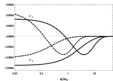
Figure 2: (top) Linear-log plot of the net momentum fluxes $P_{W}^{x}(u)$ and $P_{W}^{z}(u)$ for $\alpha=0.2$ (dashed curves) and $\alpha=0.5$ (continuous curves). For both cases, an initial regime of positive momentum flux along the $z$ axis is present. The main contribution to the associated impulse comes from the final dominant deceleration phase. (bottom) Plot of the gravitational wave impulses associated with the net momentum fluxes for $\alpha=0.2$ on top. Both curves tend to a constant negative value, when the gravitational wave emission ceases.

The behavior of the impulse is illustrated in Fig. 2 (bottom) for the case $\alpha=0.2$ of Fig. 2 (top). As expected the curve for $I_{W}^{z}(u)$ presents a local maximum, when the area measured below the curve of $P_{W}^{z}(u)$ starts to give a negative contribution to the impulse. For large $u\sim u_{f}$ both curves tend to a constant negative value, corresponding to the final configuration of the system. Fig. 2 (bottom) also illustrates the dominance of the deceleration regime in the processes. The plateau is considered to be reached when $|{\bf I}_{W}(u)-{\bf I}_{W}(u+h)|\lesssim 10^{-10}$, where $h$ is the stepsize of the integration used for the evaluation of ${\bf I}_{W}(u)$. At this stage the remnant black hole has a momentum ${\bf P}_{f}\equiv{\bf P}(u_{f})=(n_{1f},0,n_{3f})~{}P_{f}$, with

$$P_{f}=m_{0}K_{f}^{3}\sinh\gamma_{f},$$ (20)

whose distribution as function of $\alpha$, for several $\rho_{0}$, is given in [24]. Table 3 contains data characterizing ${P}_{f}/m_{0}$ in the case $\rho_{0}=21^{\circ}$.

From Eq. (18) we can derive that

$$P^{x}(u_{f})-P^{x}(u_{0})=I^{x}_{W}(u_{f}),~{}~{}P^{z}(u_{f})-P^{z}(u_{0})=I^{z}_{W}(u_{f}),~{}~{}$$ (21)

where the right-hand sides of (21) are the nonzero components of the net total impulse ${\bf I}_{W}(u_{f})$. We remark that for larger values of $\alpha$, the final impulse $I_{W}^{x}(u_{f})$ is larger than $I_{W}^{z}(u_{f})$, contrary to the cases $\alpha=0.2,~{}0.5$. This is shown in Figs. 3 where we plot the net momentum fluxes $P_{W}^{x}(u)$ and $P_{W}^{z}(u)$, and the associated impulses $I_{W}^{x}(u)$ and $I_{W}^{z}(u)$, for the case $\alpha=1$.

The purpose of Figs. 3 is two-fold. First to show that, for high values of the mass ratio, the initial phase of positive gravitational wave flux along the $z$-axis is absent, with an overall deceleration of the merged system during the whole regime of gravitational wave emission, typical of gravitational bremsstrahlung. Second, the total final impulse along the $z$ axis is about one order of magnitude smaller than the total impulse along the $x$ axis; both of them are at least one order of magnitude larger than the corresponding impulses for $\alpha=0.2$. We should also note that in this case $\alpha=1$ (initial data corresponding to equal-mass black holes) the net gravitational wave flux and the associated impulse are nonzero. This is not in contradiction with numerical relativity results for binary black hole inspirals since only the case of a head-on collision ($\rho_{0}=0^{\circ}$ in our data (15)) can approximate, and therefore be compared with the post-merger phase of black hole binary inspirals. Actually our initial data with $\rho_{0}=0^{\circ}$ yields a zero net momentum flux for $\alpha=1$ as expected (cf. also [32]). In this sense the results of Table 3 (cf. also Fig. 4) should be interpreted in the light of gravitational configurations emitting gravitational waves other than black hole binary inspirals. Since, to our knowledge, all black hole spacetimes examined in the literature of numerical relativity correspond either to binary black hole inspirals or to head-on collisions we have presently no reference for comparison or analogy with our results. Our best guess is that this system might be a candidate to an approximate description of the post-merger phase of a non-head-on collision of black holes not preceded by a pre-merger inspiral phase, as for instance colliding black holes in pre-merger unbounded trajectories as schematically illustrated in Fig. 1. Such a system reminds us of the near encounters of two bodies along unbounded trajectories that were treated in Refs. [33] where the authors, using a post-Newtonian treatment, showed the universality of gravitational bremsstrahlung for these systems. However the use of black hole initial conditions and distinct incidence angles, as well as a possible merger, were not contemplated in their treatment due to the approximations used.

Table 3: Summary of our numerical results corresponding to an initial boost parameter $\gamma=0.5$ and incidence angle $\rho_{0}=21^{\circ}$.

$\alpha$	$\eta$	$K_{f}$	$v_{f}/c=\tanh\gamma_{f}$	$\rho_{f}$	$-I_{W}^{x}(u_{f})/m_{0}$	$-I_{W}^{z}(u_{f})/m_{0}$	$V_{k}~{}({\rm km/s})$
$0.025$	$0.0238$	$1.045113$	$0.446425$	$0.37^{\circ}$	$1.2792\times 10^{-6}$	$8.1563\times 10^{-6}$	$2.17$
$0.050$	$0.0453$	$1.091454$	$0.430866$	$0.77^{\circ}$	$5.6819\times 10^{-6}$	$3.3361\times 10^{-5}$	$7.80$
$0.100$	$0.0826$	$1.187836$	$0.400255$	$1.65^{\circ}$	$2.7635\times 10^{-5}$	$1.3834\times 10^{-4}$	$25.25$
$0.150$	$0.1134$	$1.289162$	$0.370480$	$2.64^{\circ}$	$7.4349\times 10^{-5}$	$3.1932\times 10^{-4}$	$45.91$
$0.200$	$0.1388$	$1.395446$	$0.341701$	$3.77^{\circ}$	$1.5575\times 10^{-4}$	$5.7681\times 10^{-4}$	$65.96$
$0.250$	$0.1600$	$1.506701$	$0.314042$	$5.06^{\circ}$	$2.8314\times 10^{-4}$	$9.0763\times 10^{-4}$	$83.39$
$0.300$	$0.1775$	$1.622933$	$0.287600$	$6.53^{\circ}$	$4.6910\times 10^{-4}$	$1.3051\times 10^{-3}$	$97.33$
$0.400$	$0.2040$	$1.870356$	$0.238634$	$10.17^{\circ}$	$1.0733\times 10^{-3}$	$2.2569\times 10^{-3}$	$114.58$
$0.500$	$0.2222$	$2.137755$	$0.195219$	$15.06^{\circ}$	$2.0929\times 10^{-3}$	$3.3174\times 10^{-3}$	$120.45$
$0.525$	$0.2257$	$2.207669$	$0.185282$	$16.53^{\circ}$	$2.4287\times 10^{-3}$	$3.5817\times 10^{-3}$	$120.66$
$0.600$	$0.2344$	$2.425151$	$0.157731$	$21.77^{\circ}$	$3.6700\times 10^{-3}$	$4.3295\times 10^{-3}$	$119.38$
$0.700$	$0.2422$	$2.732560$	$0.126756$	$31.14^{\circ}$	$5.9634\times 10^{-3}$	$5.0986\times 10^{-3}$	$115.36$
$0.800$	$0.2469$	$3.059988$	$0.103331$	$44.09^{\circ}$	$9.1477\times 10^{-3}$	$5.3968\times 10^{-3}$	$111.21$
$0.900$	$0.2493$	$3.407441$	$0.088880$	$60.85^{\circ}$	$1.3413\times 10^{-2}$	$4.9651\times 10^{-3}$	$108.45$
$1.000$	$0.2500$	$3.774920$	$0.084214$	$79.50^{\circ}$	$1.8965\times 10^{-2}$	$3.5148\times 10^{-3}$	$107.57$

Figure 3: Linear-log plot of the net fluxes of momentum $P_{W}^{x}(u)$ and $P_{W}^{z}(u)$ (top) and the associated total impulses $I_{W}^{x}(u)$ and $I_{W}^{z}(u)$ (bottom), for the case $\alpha=1$ and incidence angle $\rho_{0}=21^{\circ}$.

IV.2 The total momentum and the kick velocity for non-head-on collisions

We define the net kick velocity ${\bf V}_{k}$ of the merged system as proportional to the momentum imparted to the system by the total impulse of gravitational waves. This definition is based on the impulse function ${\bf I}_{W}(u)$ of the gravitational waves evaluated at $u=u_{f}$ (cf. Eqs. (21)) and are in accordance with [10]. We obtain (restoring universal constants)

$${\bf V}_{k} = \frac{c}{m_{0}K_{f}^{3}}~{}{\bf I}_{W}(u_{f}),$$ (22)

with modulus

$$V_{k}=\frac{c}{m_{0}K_{f}^{3}}~{}\sqrt{I_{W}^{x}(u_{f})^{2}+I_{W}^{z}(u_{f})^{2}}~{},$$ (23)

where $m_{0}K_{f}^{3}$ is the rest mass of the remnant black hole. Taking into account the momentum conservation equations (18) evaluated at $u=u_{f}$ we interpret the definition (22) as the balance between the Bondi momentum of the system and the impulse of the gravitational waves in a zero-initial-Bondi-momentum frame, which can then be compared with the results of the existing literature. We remark that the zero-initial-Bondi-momentum frame is the inertial frame related to the asymptotic Lorentz frame used in our computations by a velocity transformation with velocity parameter ${\small{\bf v}_{B}={\bf P}(u_{0})/m_{0}K_{f}^{3}}$ ; in the parameter domain of our numerical experiments the relativistic corrections in this transformation may be neglected.

We evaluate $V_{k}$ for several values of $\alpha$, for fixed $\gamma=0.5$ and incidence angle $\rho_{0}=21^{\circ}$. The results are summarized in Table 3 where we use the symmetric mass parameter $\eta=\alpha/(1+\alpha)^{2}$. In Fig. 4 we plot the points $(V_{k},\eta)$ from Table 3. The continuous curve is the least-square-fit of the points to the empirical analytical formula,

$$V=A\eta^{2}(1-4C\eta)^{1/2}(1+B\eta)\times 10^{3}~{}{\rm km/s},$$ (24)

with best fit parameters $A\simeq 3.63538199$, $B\simeq 2.46152380$ and $C\simeq 0.91379025$. The maximum net antikick obtained is $\simeq 120.66~{}{\rm km/s}$ at $\eta\simeq 0.2257$.

Figure 4: Plot of the points ($V_{k},\eta$) given in Table 3, for $\rho_{0}=21^{\circ}$. The continuous curve is the best fit of the points to the empirical law (24). The maximum of the curve corresponds to $V_{k}\simeq 120.66~{}{\rm km/s}$ for $\eta\simeq 0.2257$ ($\alpha\simeq 0.5249$). The normalized rms error of the fit is $\simeq 0.13\%$. The nonzero kick for $\alpha=1$ confirms that the non-head-on initial data have no connection with black hole binary inspirals.

The parameter $C$ is empirically introduced to account for the nonzero kick velocity in the non-head-on case with mass ratio $\alpha=1$. We note that (24) reduces to the Fitchett law[34, 6] for $C=1$. We must emphasize that the results shown in Fig. 4 have no connection with black hole binary inspirals, as discussed already, rather possibly with two colliding black holes in pre-merger unbounded trajectories as schematically shown in Fig. 1. We note however that our data (15) for $\rho_{0}=0^{\circ}$ (head-on case) yield a Fitchett distribution, as expected and discussed in the next subsection.

The nonzero kick velocity for the non-head-on data with $\alpha=1$ and $\rho_{0}=21^{\circ}$ deserves a more detailed discussion. In this case we can evaluate the components of the initial Bondi-Sachs momentum to be, $P^{x}(0)/m_{0}\simeq 4.489093$, $P^{z}(0)/m_{0}\simeq 0.832004$ and $P^{y}(0)/m_{0}\simeq 0$, with respect to an asymptotic Lorentz observer. This momentum vector, which lies in the right quadrant of the upper hemisphere $z>0$ of the plane $x-z$, makes an angle $\Theta_{B}=\arctan|P^{x}(0)/P^{z}(0)|\simeq 1.387537$ radians (or $\Theta_{B}\simeq 79.5^{\circ}$) with the positive $z$-axis. This is also the direction of the nonzero momentum of the remnant with respect to the same asymptotic Lorentz frame, determined by the angle $\rho_{f}$, which satisfies $\rho_{f}=(180^{\circ}-\rho_{0})/2$ for $\alpha=1$ and any $\rho_{0}$ (cf. Table 3 and Ref. [24]). The axis determined by $\rho_{f}\equiv\Theta_{B}$ actually plays an important role in the dynamics. If we take a new frame with its $z$-axis coinciding with this axis the net gravitational wave momentum flux vector ${\bf P}_{W}(u)$ lies along the new $z$-axis for all $u$. This was verified numerically by evaluating the ratios of the computed fluxes, used to construct Fig. 3 (right), sampled in the interval $0<u/m_{0}\leq 890$, yielding in all cases $\arctan|I_{W}^{x}(u)/I_{W}^{z}(u)|\simeq 1.387541$ with a relative error of the order of $10^{-6}$. Still in this new frame the data will not be symmetric under $\theta\rightarrow\pi-\theta$, leading to a nonzero net gravitational wave momentum flux, contrary to the case of merging binary inspirals and head-on collisions. As expected the $z$-axis of the new frame is the direction of the kick velocity since $\arctan|I_{W}^{x}(u_{f})/I_{W}^{z}(u_{f})|\simeq 1.387547~{}{\rm rad}$ or $\simeq 79.5^{\circ}$ (within the precision of data in Table 3). Finally in the evolution of these data we had no evidence of the presence of a junk radiation component, as discussed already. Therefore it is unlikely that the nonzero net gravitational wave momentum flux in this case is a contribution of a junk radiation component.

Figure 5: Plot of the integral curve ${\bf x}(u)$ of the wave impulse vector field ${\bf I}_{W}(u)$ which can give a schematic picture of the motion of the system in the zero-momentum-Bondi frame, for $\alpha=0.2$ and $\rho_{0}=21^{\circ}$. The asymptote of the curve as $u\rightarrow u_{f}$ makes an angle $\Theta_{f}\simeq 15.11^{o}$ with the negative $z$-axis of this frame.

In general, in a zero-initial-Bondi-momentum frame, the Bondi momentum of the merged system satisfies ${\bf P}(u)={\bf I}_{W}(u)$ so that an integral curve ${\bf x}(u)$ of the wave impulse vector field ${\bf I}_{W}(u)$, defined as $d{\bf x}/du={\bf P}(u)$, can give a schematic picture of the motion of the merged system in this frame. In Fig. 5 we display this integral curve for $\alpha=0.2$ and $\rho_{0}=21^{\circ}$, generated with initial conditions $x(u_{0})=0=z(u_{0})$ in the zero-initial-Bondi-momentum frame. The initial phase of positive momentum flux along $z$ is responsible for the curved form of the trajectory in the semiplane $z>0$. For $u\rightarrow u_{f}$ the curve approaches the asymptote with angle $\Theta_{f}=\arctan(I_{W}^{x}(u_{f})/I_{W}^{z}(u_{f}))\simeq 15.11^{\circ}$ with respect to the negative $z$-axis of the zero-initial-Bondi-momentum frame, which is actually the direction of the kick velocity in this frame. In the case $\alpha=1$ the integral curve is a straight line with angle $\Theta_{f}\simeq 79.5^{\circ}\equiv(180^{\circ}-21^{\circ})/2$ with respect to the $z$-axis of the zero-initial-Bondi-momentum frame (cf. Table 3).

IV.3 Head-on kick distributions: a comparison to results of the literature

We now compare and discuss our evaluations of kick velocities for the head-on case ($\rho_{0}=0^{\circ}$) with the results of the numerical relativity simulations (bridged with analytical approximations) of Refs. [15] (PN+CLA) and [7] (CLA), and with results of full numerical relativity of Refs. [2, 10, 11, 13, 14]. These works treat black hole inspiral binary systems and are related to our results in the sense that head-on collisions can be an approximation model to the final plunge to merger in binary inspirals. The kick distribution obtained in our simulations satisfies the Fitchett law (cf. also [32]), so that the recoil evaluated from the BS net momentum fluxes can give a complementary information on the momentum extraction, contributing to the understanding of the processes of producing kicks and anti-kicks. The post-merger phase corresponding to our head-on initial data exhibits two distinct regimes, an initial positive, followed by a dominant negative phase of net momentum flux, a pattern consistent with kick and antikick contributions.

For our numerical experiments in this subsection we have adopted an initial data with boost parameter $\gamma=0.56$, chosen to match the maximum kick velocity of [15]. The results are displayed in Fig. 6 together with the main results of Refs. [2, 7, 10, 11, 13, 14, 15]. The points $(V_{k},\eta)$ of our simulations are fitted by the Fitchett law $V_{k}=A\eta^{2}(1-4\eta)^{1/2}(1+B\eta)\times 10^{3}~{}{\rm km/s}$, with best fit parameters $A=5.4719439$ and $B=3.874397$. The normalized rms of the fit to the points is $\simeq 0.36\%$. The results of the PN+CLA[15] are shown by their Fitchett curve, fitted with parameters $A=9.5$ and $B=0.3$, and four points with error estimates. The CLA treatment of [7] is given by the curve $V_{k}=11.292\eta^{2}(1-4\eta)^{1/2}(1-1.6070\eta+1.9076\eta^{2})\times 10^{3}~{}{\rm km/s}$. The full numerical relativity calculations of González et al.[10] are given by the Fitchett curve fitted with parameters $A=12$, $B=-0.93$, with a maximum kick $V_{k}=175.2\pm 11{\rm km/s}$ at $\eta=0.195\pm 0.005$. The agreement of our numerical results with the corresponding points of numerical relativity simulations is to $5\%-8\%$ for the range of mass ratios $0.3\leq\alpha\leq 0.95$. Larger discrepancies occur for smaller mass ratios, of the order of $15\%-31\%$. These systematic discrepancies could possibly be due to a missing inspiral contribution since the RT dynamics covers only the post-merger phase of the system. However, in spite of these discrepancies, our results confirm that the main contribution to the kicks comes from the post merger phase.

A full numerical relativity treatment of the gravitational wave recoil in head-on collisions of two black holes was done in Choi et al.[16], where both the black hole mass ratio and spins are varied. For the unequal mass case ($\alpha=0.667$) without spin they obtained a net kick velocity $V_{k}\sim 2.76~{}{\rm km/s}$, for a large initial separation ($L/M=12.24$) with the black holes starting at rest. The latter two conditions of the initial configuration can possibly be the reason for the discrepancy of two orders of magnitude with our result for the same mass ratio, which is $V_{k}\sim 121~{}{\rm km/s}$ (for $\gamma=0.56$) and $V_{k}\sim 70~{}{\rm km/s}$ (for $\gamma=0.5$). In fact we have evaluated the net kick for a sufficiently small value $\gamma=0.26$ and the same mass ratio $\alpha=0.667$ in our data. We obtained $V_{k}\simeq 2.59~{}{\rm km/s}$, of the order of their reported value. The paper [16] does not provide values of kicks for other mass ratios, which would be a valuable comparison to our results in the BS approach.

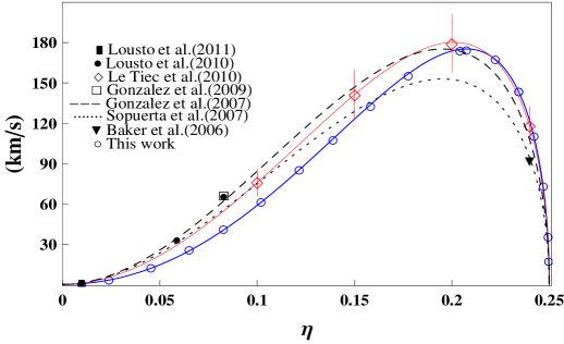
Figure 6: Comparing our numerical results for kicks generated in the post-merger phase of a head-on collision with CLA[7] and PN+CLA[15] results, and with full numerical relativity results[2, 10, 11, 13, 14] for binary black hole mergers.

Finally we refer to the works of Shibata et al.[35] and Sperhake et al.[36] examined the collision of two equal black holes, with anti-parallel initial velocities, directed at each other with an impact parameter. We consider that the initial data used by the authors do not actually describe the same physical situation of our non-head-on data. In our case, for any value of the incidence angle $\rho_{0}$, a black hole is formed while in those authors’ data this depends on the impact parameter, with a critical threshold for the formation of black holes. Furthermore they report a huge increase in the efficiency of energy extraction by gravitational waves as compared to the case of zero impact parameter (pure head-on). In contrast, in our system, head-on collisions constitute an upper bound for the efficiency. The efficiency decreases monotonically with the increase of $\rho_{0}$ for any $\alpha$, as examined in Ref. [24]. Therefore there appears to be no obvious connection between the impact parameter $b$ of their data and the parameter $\rho_{0}$ of our initial data.

V Final Discussions and Conclusions

The present paper extends our work in [24] by examining the gravitational wave recoil in non-axisymmetric Robinson-Trautman spacetimes in the BS characteristic formalism. The initial data already have a common apparent horizon so that the RT dynamics actually evolves a distorted black hole, reminiscent of the CLA approach[25, 26]. The characteristic initial data used in the RT dynamics were derived and interpreted in [24] as corresponding to the early post-merger state of two boosted colliding black holes with a common apparent horizon. The basic parameters of the initial data are the mass ratio $\alpha$, the boost parameter $\gamma$ and the incidence angle $\rho_{0}$. Head-on collisions correspond to the particular case $\rho_{0}=0^{\circ}$ and only in this case can our results be compared with numerical relativity calculations for binary black hole spacetimes and head-on collisions. Our analysis is based on the Bondi-Sachs momentum conservation laws that regulate the radiative transfer processes of the system. We use a numerical code based on the Galerkin spectral method[24], which is sufficiently accurate and stable for long time runs, and we evaluate the parameters of the remnant black hole, the gravitational wave net momentum fluxes and the impulse imparted to the system by the emitted radiation.

In the paper we restricted our numerical computations to two distinct sets of initial data: (i) initial data corresponding to a non-head-on collision with $\rho_{0}=21^{\circ}$, and $\gamma=0.5$ fixed; (ii) initial data corresponding to head-on collisions ($\rho_{0}=0^{\circ}$ ) and $\gamma=0.56,~{}0.26$, the values of $\gamma$ being adopted in order to compare our simulations with numerical relativity simulations of inspiral black hole binaries. A feature to be remarked in the case of non-head-on initial data (i) is the nonzero net gravitational wave flux for equal mass black holes, contrary to the case of head-on collisions and inspiral black hole binaries, showing that the data (i) has no connection or analogy with black hole binary inspirals and head-on collisions examined in numerical relativity simulations. We suggest that these data might be a candidate to an approximate description of a post-merger phase of a non-head-on collision of black holes in unbounded trajectories. The numerical results for the head-on initial data (ii) were compared with published results of kick distributions in numerical relativity, as from PN+CLA[7, 15] to numerical relativity evaluations[2, 10, 11, 13, 14] of kicks in the collapse and merger of nonspinning black hole binaries. This comparison is made taking into account that a head-on configuration may be seen as an approximation to the final plunge to merger of inspiral binaries. For the range of mass ratios $(0.3\leq\alpha\leq 0.95)$ we have an agreement to $5\%-8\%$, but larger discrepancies occur for smaller mass ratios. Our results confirm that the post merger phase gives a substantial contribution to the kicks.

The full numerical relativity experiment of Choi et al.[16] for head-on collisions of nonspinning black holes obtained a kick velocity two orders of magnitude smaller then the ones reported in our results shown in Fig. 6. We evaluated the net kick velocity using the same mass ratio but a smaller boost parameter to approach their initial data that used black holes starting at rest. We obtained a kick of the same order. Finally we discussed Refs. [35, 36], where the collision of two equal-mass black holes with an impact parameter is examined, and compared with our non-head-on case. The authors report a huge increase in the efficiency of energy extraction as compared to the case of zero impact parameter (pure head-on). In contrast, in our system, head-on collisions $(\rho_{0}=0^{\circ})$ constitute an upper bound for the efficiency, which decreases monotonically with the increase of $\rho_{0}$[24]. Therefore there appears to be no obvious connection between the impact parameter of their data and the parameter $\rho_{0}$ of our initial data.

References

- [1] F. Pretorius, Physics of Relativistic Objects in Compact Binaries: from Birth to Coalescence, Eds. Colpi M, Casella P, Gorini V, Moschella U and Possenti A, (Astrophysics and Space Science Library Series, Vol. 359, Springer, Heidelberg), p. 305 (2009).
- [2] J. B. Baker, J. Centrella, D. Choi, M. Koppitz, M. van Meter and M. C. Miller, Astrophys. J. 653 L93-L96 (2006).
- [3] D. Merrit, M. Milosavljević, M. Favata, S. S. Hughes and D. E. Holz, Astrophys. J. 607 L9 (2004).
- [4] M. Favata M, S. A. Hughes and D. E. Holz, Astrophys. J. 607 L5 (2004).
- [5] S. Komossa, H. Zhou and H. Lu , Astrophys. J. 678 L81 (2008); P. G. Jonker, M. A. P. Torres, A. C. Fabian, M. Heida, G. Miniutti and D. Pooley, Mon. Not. R. Astron. Soc 407 645 (2010).
- [6] L. Blanchet, M. S. S. Qusailah and C. M. Will, Astrophys. J. 635 508 (2005).
- [7] C. F. Sopuerta, N. Yunes and P. Laguna, Phys. Rev. D 74 124010 (2006); Erratum: Phys. Rev. D 75 069903(E) (2007).
- [8] J. A. González, M. Hannam, U. Sperhake, B. Brügmann and S. Husa, Phys. Rev. Lett. 98 091101 (2007).
- [9] M. Campanelli, C. O. Lousto, Y. Zlochower and D. Merritt, Astrophys. J. 659 L5-L8 (2007).
- [10] J. A. González, U. Sperhake, B. Brügmann, M. Hannam and S. Husa, Phys. Rev. Lett. 98 091101 (2007).
- [11] J. A. González, U. Sperhake and B. Brügmann, Phys. Rev. D 79 124006 (2009).
- [12] C. O. Lousto, N. Nakano, Y. Zlochower Y and M. Campanelli, Phys. Rev. Lett. 104 211101 (2010).
- [13] N. Nakano, Y. Zlochower, C. O. Lousto and M. Campanelli, Phys. Rev. D 84 124006 (2011).
- [14] C. O. Lousto Y. Zlochower, Phys. Rev. Lett. 106 041101 (2011).
- [15] A. Le Tiec, L. Blanchet and C. M. Will, Class. Q. Grav. 27 012001 (2010).
- [16] D. Choi, B. J. Kelly, W. D. Boggs, J. G. Baker, J. Centrella and J. van Meter Phys. Rev. D 76 104026 (2007).
- [17] L. Rezzolla, R. P. Macedo and J. L. Jaramillo, Phys. Rev. Lett. 104 221101 (2010).
- [18] J. L. Jaramillo, R. P. Macedo, P. Moesta and L. Rezzolla, Phys. Rev. D 85 084030 (2012).
- [19] R. F. Aranha, I. Damião Soares and E. V. Tonini, Phys. Rev. D 81 104005 (2010).
- [20] R. F. Aranha, H. P. Oliveira, I. Damião Soares and E. V. Tonini, Int. J. Mod. Phys. D 17 2049 (2008).
- [21] I. Robinson and A. Trautman, Phys. Rev. Lett. 4 431 (1960); I. Robinson and A. Trautman, Proc. Roy. Soc. London A 265 463 (1962).
- [22] H. Bondi H, M. G. J. van der Berg and A. W. K. Metzner, Proc. Roy. Soc. London A 269 21 (1962).
- [23] R. K. Sachs, Proc. Roy. Soc. London A 270 103 (1962); R. K. Sachs, J. Math. Phys. 3 908 (1962).
- [24] R. F. Aranha, I. Damião Soares and E. V. Tonini, Phys. Rev. D 85 024003 (2012).
- [25] F. Zerilli, Phys. Rev. Lett. 24 737 (1970); C. T. Cunningham, R. H. Price and V. Moncrief, Astrophys. J. 224 643 (1978).
- [26] S. A. Teukolsky, Phys. Rev. Lett. 29 1114 (1972).
- [27] P. Chrusciel, Commun. Math. Phys. 137 289 (1991); P. Chruściel P and D. B. Singleton, Commun. Math. Phys. 147 137 (1992).
- [28] K. P. Tod, Class. Quantum Grav. 6 1159 (1989); H. P. Oliveira, E. Rodrigues and I. Damião Soares, Braz. J. Phys. 41 314 (2011).
- [29] R. K. Sachs, Phys. Rev. 128 2851 (1962).
- [30] R. F. Aranha, I. Damião Soares and E. V. Tonini, Class. Quantum Grav. 30 025014 (2013).
- [31] C. A. Fletcher, Computational Galerkin Methods (Berlin: Springer-Verlag, 1984).
- [32] R. F. Aranha, I. Damião Soares and E. V. Tonini, Phys. Rev. D 82 104033 (2010).
- [33] P. C. Peters, Phys. Rev. D 1 1557 (1970); M. Turner, Astrophys. J. 216 610 (1977); S. D. Kovács and K. S. Thorne, Astrophys. J. 217 252 (1977); M. Turner and C. W. Will, Astrophys. J. 220 1107 (1978); S. D. Kovács and K. S. Thorne, Astrophys. J. 224 62 (1978).
- [34] M. J. Fitchett, Mon. Not. R. Astron. Soc. 203 1049 (1983).
- [35] M. Shibata, H. Okawa and T. Yamamoto, Phys. Rev. D 78 101501 (2008).
- [36] U. Sperhake, V. Cardoso, F. Pretorius, E. Berti, T. Hinderer and N. Yunes, Phys. Rev. Lett. 103 131102 (2009).