Spectral properties of attractive bosons in a ring lattice including a single-site potential

Abstract

The ground-state properties of attractive bosons trapped in a ring lattice including a single attractive potential well with an adjustable depth are investigated. The energy spectrum is reconstructed both in the strong-interaction limit and in the superfluid regime within the Bogoliubov picture. The analytical results thus obtained are compared with those found numerically from the exact Hamiltonian, in order to identify the regions in the parameter space where this picture is effective. The single potential introduced is the simplest way to break the translational symmetry and to observe, through a completely analytical approach, how the absence of symmetry affects the properties of the low-excited eigenstates of the system. This model gives a first insight into the properties of systems including more complex potentials.

1 Introduction

Attractive bosons trapped in a one-dimensional (1D) periodic lattice [1]-[5] or in mesoscopic arrays [6]-[10] have recently received considerable attention because they provide a natural framework where Schrödinger-cat states [11]-[13] are in principle observable. Both the ground state and low-energy states of these systems, in fact, have been shown to consist of superpositions of macroscopic spatially-localized quantum states when the boson-boson interaction is sufficiently strong. Meanwhile, a stimulating experimental work has made concrete the realizability of lattices with a ring geometry [14] and the development of optical-trapping schemes for engineering mesoscopic arrays [15], [16] in which Feshbach resonances [17] ensure a full control of boson-boson interaction. $N$ bosons in a 1D periodic $M$-site lattice are well described within the Bose-Hubbard picture by model Hamiltonian [18], [19]

$$H=\frac{\cal U}{2}\sum_{j}(n_{j}^{2}-n_{j})-V-T\sum_{j}(a_{j+1}^{+}a_{j}+a_{j+1}a^{+}_{j})\,,$$ (1)

where $n_{i}=a^{+}_{i}a_{i}$ ($i=1,...,M$), $a_{i+M}=a_{i}$ and $a_{i}$, $a^{+}_{i}$ obey the standard commutators $[a_{m},a^{+}_{i}]=\delta_{mi}$. The boson tunneling among the lattice potential wells and boson-boson interactions are described by means of the hopping amplitude $T$ and parameter ${\cal U}<0$ (${\cal U}>0$), respectively, in the attractive (repulsive) case. In addition, term $V=\sum_{i}V_{i}\,n_{i}$ includes local potentials with well depths $V_{i}$ thus giving the possibility to represent disordered lattices and/or trapping potentials.

If $v_{i}=0$ for each $i$, the resulting system is homogeneous and features translation invariance. For ${\cal U}<0$, the relevant zero-temperature scenario has been investigated in [2] and [5] showing how the resulting delocalized ground state exhibits three characteristic regimes depending on the value of $\tau=T/(|{\cal U}|N)$. In the strong-interaction (SI) regime, where $\tau<\tau_{1}\simeq 1/4$, the ground state is a Schrödinger cat well represented by a super-position of $M$ coherent states of algebra su($M$), each one describing the strong localization of bosons around a given lattice site. The opposite weak-interaction regime is the superfluid (SF) one, defined in the open interval $\tau>\tau_{2}$ $=1/[2M\sin^{2}(\pi/M)]$. Its ground state reduces to a single su($M$) coherent state describing the uniform distribution of bosons in the lattice and, thus, their complete delocalization. Last, for $\tau_{1}<\tau<\tau_{2}$, the solitonlike regime features a ground state which again is a superposition of $M$ localized states. The latter, however, exhibit an intermediate character: their localization peaks describe boson distributions involving a significant number of lattice sites. Peaks become sharper and sharper when $\tau\to\tau_{1}$.

This almost ideal scenario, where translation invariance combined with the fact that ${\cal U}<0$ enable Schrödinger-cat states to appear, breaks up as soon as $V\neq 0$. In this paper we investigate the low-energy properties of model (1) and analyze, in particular, the crucial role played by a localized perturbation, a single potential well, in modifying the structure of low-energy states and the relevant spectrum. The interest for this model is supported by various motivations. First, the introduction of a local potential well is the simplest possible way to introduce a disturbance in a perfectly symmetric ring lattice characterized by translation invariance. Potential $V$ in $H$ will contribute with a single term at some site $j$ and $V_{i}=0$ for any $i\neq j$. Moreover, this naive model preludes to a very realistic situation. In fact, the presence of lattice defects –representable in terms of extremely weak local potentials– should be viewed as an intrinsic, essentially uncontrollable, ingredient of the experimental setup. If ${\cal U}>0$, their perturbative character does not affect large-scale phenomena such as the formation of Mott and SF states and thus defects can be ignored. Conversely, for ${\cal U}<0$, a single, even vanishingly small, defect is able to break the system symmetry therefore preventing the formation of Schrödinger cats. Finally, the model with a single-site potential has the non secondary advantage to allow one the implementation of standard approximation schemes and a fully analytic study of the Hamiltonian and of its energy spectrum.

We show that, in the SI regime and in the presence of a single potential well (placed, for example, at $j=0$) with depth $V_{0}$ even arbitrarily small, the localization effect of bosons enables us to operate a remarkable simplification of $H$. The latter reduces to a pure-hopping model including a new effective local potential whose depth is proportional to the total boson number (and therefore is much larger than $V_{0}$). Such a new form is particularly useful since, with essentially no analytic work, $H$ can be separated in two commuting sub-Hamiltonians one of which is intrinsically diagonal. The most interesting feature, however, concerns the SP (single-particle) energy spectrum obtained from the complete diagonalization of $H$. Depending on the choice of parameters $T$, $\cal U$ and $V_{0}$, the spectrum exhibits a structure characterized either by well-visible energy doublets or by an almost uniform distribution of SP energies. The notable exception in the latter case is the lowest SP energy showing, for $\tau\to 0$, an unexpected diverging behavior to arbitrarily large negative values. This feature has been already observed in the study of the SP spectrum of bosonic comb lattices [20] and of their unusual zero-temperature properties.

Then we investigate the SF regime by adopting the standard Bogoliubov picture to recast our $V\neq 0$ model into a more convenient form. In this case, however, a rather hard mathematical work is necessary to diagonalize $H$. To this end, after recognizing that $H$ can be expressed as a linear combination of the operators belonging to $M$ independent su(1,1)-like algebras, a remarkable help in the diagonalization process comes from exploiting the transformation properties of such algebras. Also in this case, the definition of two independent sets of new bosonic modes makes $H$ separable into two commuting sub-Hamiltonians one of which exhibits the characteristic SP energies distinguishing the solution of SF models within the Bogoliubov diagonalization scheme. The SP energies of the other sub-Hamiltonian (this is written in terms of $V_{0}$-dependent modes) are found to represent small deviations of Bogoliubov-like SP energies. The SP spectrum is thus characterized by energy doublets. Both in the SI and in the SF case, we determine the analytic form of weakly excited states.

Sections II and III are devoted to the study of the SI regime and the SF regime, respectively. In both sections the validity of analytic results concerning the ground state and the first few weakly-excited energy levels are compared with numerical results. Section IV is devoted to final comments.

2 Low-energy states in the SI regime

Low-energy states of Hamiltonian (1) with $V=0$ and ${\cal U}<0$ consist of a superposition of su($M$) coherent states, each one involving a boson distribution strongly localized around a different site of the lattice. Such coherent states are defined by

$$|\xi\rangle\,:=\frac{1}{\sqrt{N!}}\left(\sum^{M-1}_{i=0}\xi_{i}a^{+}_{i}\right)^{N}|0\rangle\,,\quad\langle\eta|\xi\rangle=\left(\sum^{M-1}_{m=0}\eta^{*}_{m}\xi_{m}\right)^{N}$$

where $N$ is the total boson number, state $|0\rangle$ is such that $a_{i}|0\rangle=0$ for each $i$, and the second equation defines the scalar product of two generic states. The normalization of $\langle\xi|\xi\rangle$ is thus ensured by $\sum_{m}\xi^{*}_{m}\xi_{m}=1$. Based on the previuos definition, the explicit form of low-energy states in terms of localized states $|\xi(j)\rangle$ was found to be [2]

$$|E_{k}\rangle=\sum^{M-1}_{j=0}\,\frac{e^{i{\tilde{k}}j}}{\sqrt{M}}\,|\xi(j)\rangle\,,\qquad|\xi_{i}(j)|<<|\xi_{j}(j)|\simeq 1$$ (2)

in which index ${\tilde{k}}=2\pi k/M$ with $k\in[0,M-1]$ essentially represents the eigenvalue of the quasi-momentum operator generating lattice translations. The ground state corresponds to the case $k=0$. The localization of bosons at site $j$ is embodied in inequality $|\xi_{i}(j)|<<|\xi_{j}(j)|$ of formula (2), the quantity $|\xi_{\ell}(j)|^{2}$ representing the fraction of population at site $\ell$ according to state $|\xi(j)\rangle$. This feature becomes evident by reminding that $\langle\xi(j)|a^{+}_{\ell}a_{\ell}|\xi(j)\rangle=N|\xi_{\ell}(j)|^{2}$ [21]. In addition, because states $|\xi(j)\rangle$ can be equipped with the property $\langle\xi(i)|\xi(m)\rangle=\delta_{im}$, one can prove [21] that $\langle E_{k}|a^{+}_{i}a_{i}|E_{k}\rangle=N/M$ whose site independence confirms that $|E_{k}\rangle$ are delocalized states. For $\tau<1/4$, states $|E_{k}\rangle$ have been shown [2] to provide a quite satisfactory approximation of the true energy eigensates whose exact form can be found only numerically.

In the ideal lattice ($V=0$) the model features translation symmetry which is responsible for the super-position of equal-weight localized states in state (2). In the classical limit, this symmetry is broken: only one of components $|\xi(j)\rangle$ survives giving rise to the exponential localization [22] that is known to distinguish the maximally excited state of model (1) with ${\cal U}>0$. The presence of local potential $V=V_{0}n_{0}$ ($V_{0}>0$) in our quantum model

$$H=-\frac{U}{2}\sum_{i}n_{i}(n_{i}-1)-V_{0}n_{0}-T\sum_{i}(a^{+}_{i+1}a_{i}+\mathrm{H.C.})$$ (3)

with ${\cal U}=-U<0$ also breaks this symmetry suggesting that only one among the $M$ components of $|E_{0}\rangle$ is expected to survive. If one assumes that the most part of the population is placed at site $j=0$ owing to the presence of the attractive well, then Hamiltonian (3) can be taken into a new approximate form whose diagonalization appears to be rather simple. The approximation we effect essentially coincides with the Bogoliubov scheme. Observing that $N=\sum_{i}\,n_{i}\,\Rightarrow\,n_{0}=N-\delta N$ where $\delta N={\sum_{i\neq 0}}n_{i}$ and $n_{i}<<n_{0}\simeq N$ for $i\neq 0$, then

$$\sum_{i}n_{i}^{2}={\sum_{i}}^{*}n_{i}^{2}+N^{2}+(\delta N)^{2}-2N\,\delta N\simeq-N^{2}+2N\,n_{0}$$

in which terms $n_{i}n_{m}$ with $i,m\neq 0$ have been suppressed. Model (3) thus reduces to

$$H\simeq\frac{U}{2}N(N+1)-wn_{0}-T{\sum}_{j}(a^{+}_{i+1}a_{i}+\mathrm{H.C.})$$ (4)

in which the assumed localization at $j=0$ has the dramatic effect to involve a much deeper (effective) well with depth $w=UN+V_{0}$ together with the disappearence of nonlinear interaction terms $n_{i}(n_{i}-1)$. Therefore, even if the initial well is a simple perturbation where $V_{0}$ could be vanishingly small, the depth of the resulting effective well can be really large since it depends on $UN$. The role of attractive interaction ${\cal U}=$ $-U<0$ is thus to reduce the initial model to a pure-hopping model with a deeper effective well.

2.1 Diagonalization

After assuming Hamiltonian (4) as the reference model in the SI regime, its diagonalization is performed by resorting to the momentum-mode picture

$$a_{j}=M^{-\frac{1}{2}}\sum_{k}b_{k}\,{e^{i{\tilde{k}}j}}\,\,\Leftrightarrow\,\,b_{k}=M^{-\frac{1}{2}}\sum_{k}a_{j}\,{e^{-i{\tilde{k}}j}}\,,$$ (5)

with ${\tilde{k}}=2\pi k/M$ and $j,k\in[0,M-1]$, where $a_{j+M}\equiv a_{j}$ and $b_{k}\equiv b_{k+M}$ owing to the periodic boundary conditions of the lattice. This gives

$$H_{w}=C_{N}-w\,a^{+}_{0}a_{0}-2T{\sum}_{k}\,c_{k}b^{+}_{k}b_{k}\,,$$ (6)

where $a_{0}=\sum_{k}b_{k}/{\sqrt{M}}$, $C_{N}={U}N(N+1)/2$ and $c_{k}=\cos({\tilde{k}})$. To achieve the diagonal form of $H_{w}$ it is particularly advantageous to define the new operators

$$f_{k}=(b_{k}-b_{-k})/{\sqrt{2}}\,,\quad F_{k}=(b_{k}+b_{-k})/{\sqrt{2}}\,,$$ (7)

and $F_{0}=b_{0}$, $f_{0}=0$. In case $M$ is even, the further operator $F_{M/2}=b_{M/2}$ must be included while $f_{M/2}=0$. The range of index $k$ is such that

$$1\leq k\leq S=(M-1)/2\,,\quad 1\leq k\leq S=(M-2)/2\,,$$ (8)

if $M$ is odd or even, respectively. Note that such operators satisfy the usual bosonic commutators $[f_{n},f^{+}_{h}]=\delta_{nh}=[F_{n},F^{+}_{h}]$. Then $H_{w}$ becomes

$$H_{w}=C_{N}-wa^{+}_{0}a_{0}-2T\sum^{S}_{k=1}c_{k}f^{+}_{k}f_{k}-2T\sum^{K}_{k=0}c_{k}F^{+}_{k}F_{k}$$ (9)

with

$$a_{0}={\sum}_{k}{b_{k}}/{\sqrt{M}}={\sum}^{K}_{k=0}r_{k}{F_{k}}/{\sqrt{M}}\,,$$

$r_{0}=r_{M/2}=1$, $r_{k}={\sqrt{2}}$, and the range of $k$ given by

$$0\leq k\leq K=(M-1)/2\,,\quad 0\leq k\leq K=M/2\,,$$ (10)

when $M$ is odd or even, respectively. Hamiltonian (9) is thus formed by two commuting parts one of which, $H_{f}=\frac{U}{2}N(N+1)-2T\sum^{S}_{k=1}\,c_{k}f^{+}_{k}f_{k}$, is diagonal. The remaining part,

$$H_{F}=-w\,a^{+}_{0}a_{0}-2T\sum^{K}_{k=0}\,c_{k}F^{+}_{k}F_{k}=-\sum^{K}_{h,k=0}\,L_{kh}F^{+}_{k}F_{h}\,,$$

with $L_{kh}=w\,r_{k}r_{h}/M+2Tc_{k}\delta_{kh}$, can be diagonalized in a rather direct way. In fact, since $L_{kh}$ are elements of an $M\times M$ real and symmetric matrix, there exists an orthogonal transformation of elements $B_{pk}$ such that $\sum_{p}B_{pk}B_{ph}\,=\,\delta_{kh}$, $\sum_{k}B_{pk}B_{qk}\,=\,\delta_{pq}$ and, in particular,

$${\sum}_{kh}B_{pk}L_{kh}B_{qh}\,=\,\lambda_{p}\delta_{pq}\,.$$ (11)

The latter entails $L_{kh}\,=\,\sum_{pq}B_{pk}B_{qh}\lambda_{p}\delta_{pq}$. As a result, by introducing the new bosonic creation and annihilation operators $D_{p}\,=\,\sum_{k}B_{pk}F_{k}$ and $D_{q}^{+}\,=\,\sum_{h}B_{qh}F_{h}^{+}$, satisfying standard bosonic commutators due to the orthogonality of $B_{pk}$, one gets the diagonal form

$$H_{F}\,=\,-{\sum}_{q}\lambda_{q}D^{+}_{q}D_{q}\,.$$

By using the previous definition of $L_{kh}$ together with the orthogonality relations for $B_{pk}$, equation (11) becomes $\sum_{kh}B_{pk}(wr_{k}r_{h}/M+2Tc_{k}\delta_{kh})B_{qh}=\lambda_{p}\sum_{k}B_{pk}B_{qk}$ and thus

$${\sum}_{kh}B_{pk}[w\,r_{k}r_{h}/M-(\lambda_{p}\,-\,2T\,c_{k})\delta_{kh}]B_{qh}\,=\,0\,.$$ (12)

In order to satisfy the latter equation, we define $A(p)\,=\,\sum_{h}r_{h}B_{ph}$ and impose $(\lambda_{p}-2Tc_{k})\,B_{pk}={wr_{k}}\,A(p)/{M}$ for each $p$ obtaining

$$B_{pk}=\frac{wr_{k}}{M}\,\frac{A(p)}{\lambda_{p}-2Tc_{k}}\,.$$ (13)

This definition, inserted in the orthogonality relation $\sum_{k}B_{qk}B_{qk}\,=\,1$, gives

$$|A(p)|^{2}=\frac{M^{2}}{w^{2}}\left[\,{\sum}_{k}\,\,\frac{r_{k}^{2}}{(\lambda_{q}-2Tc_{k})^{2}}\right]^{-1}\,,$$ (14)

which enables one to fix parameter $A(p)$. By multiplying both sides of (13) times $r_{k}$ and summing over $k$, one easily derives the crucial formula

$$1\,=\frac{w}{M}\,{\sum}^{K}_{k=0}\,\frac{r^{2}_{k}}{\lambda_{p}-2Tc_{k}}\,,$$ (15)

determining eigenvalues $\lambda_{p}$ and thus the $H_{F}$ spectrum. To conclude, the total (diagonal) Hamiltonian reads

$$H_{w}=C_{N}-2T{\sum}^{S}_{k=1}\,c_{k}f^{+}_{k}f_{k}-{\sum}^{K}_{q=0}\,\lambda_{q}D^{+}_{q}D_{q}\,.$$ (16)

By observing that the vacuum state of operators $f_{k}$ and $D_{p}=\sum_{k}{B}_{pk}\,F_{k}$ (these are linear combinations of $b_{k}$ and $b_{-k}$) coincides with that of modes $b_{k}$ defined by $b_{k}|0\rangle=0$ for each $k$ ($|0\rangle\equiv|0,0,\,..\,0\rangle$), the Fock states relevant to $f_{k}$ and $D_{p}$ are found to be

$$|{\vec{\ell}},{\vec{m}}\rangle=\prod^{S}_{k=1}\,\frac{(f^{+}_{k})^{\ell_{k}}}{\sqrt{\ell_{k}!}}\,\prod^{K}_{p=0}\,\frac{(D^{+}_{p})^{m_{p}}}{\sqrt{m_{p}!}}\,|0\rangle$$ (17)

satisfying $D^{+}_{q}D_{q}\,|{\vec{\ell}},{\vec{m}}\rangle=m_{q}\,|{\vec{\ell}},{\vec{m}}\rangle$ and $f^{+}_{k}f_{k}\,|{\vec{\ell}},{\vec{m}}\rangle=\ell_{k}\,|{\vec{\ell}},{\vec{m}}\rangle$. The relevant eigenvalue equation $H_{w}\,|{\vec{\ell}},{\vec{m}}\rangle=E({\vec{\ell}},{\vec{m}})|{\vec{\ell}},{\vec{m}}\rangle$ features energy eigenvalues

$$E({\vec{\ell}},{\vec{m}})=C_{N}-2T{\sum}^{S}_{k=1}\,c_{k}\ell_{k}-{\sum}^{K}_{q=0}\,\lambda_{q}m_{q}\,.$$ (18)

In particular, the ground state, in which all bosons possess the lowest SP energy $-\lambda_{0}$ and therefore $\ell_{k}=m_{q}=0$, $m_{0}=N$ (the assumption that $\lambda_{0}>\lambda_{p},\,2Tc_{k}$, $\forall\,p\neq 0$ and $\forall\,k$ will be discussed in the next section), is given by

$$|\mathrm{GS}\rangle=\frac{(D^{+}_{0})^{N}}{\sqrt{N!}}\,|0\rangle=\frac{1}{\sqrt{N!}}\left({\sum}^{K}_{k=0}{B}_{0k}\,F^{+}_{k}\right)^{N}\,|0\rangle$$ (19)

which exhibits the form of a su($M$) coherent state. This feature pertains as well to excited states such as ${(D^{+}_{p})^{N}}\,|0\rangle/{\sqrt{N!}}$ and ${(f^{+}_{k})^{N}}/{\sqrt{N!}}\,|0\rangle$ characterized by the fact that all bosons condensate in a specific single-particle energy $-\lambda_{p}$ and $-2Tc_{k}$, respectively. In the second case, however, bosons are distributed only between momentum states $+k$ and $-k$, and the total momentum turns out to be zero since $\langle b^{+}_{k}b_{k}\rangle$ = $\langle b^{+}_{-k}b_{-k}\rangle=N/2$. Any other excited state is represented by state (17).

2.2 Spectrum of $H_{w}$

Exact SP energies $-\lambda_{p}$ can be obtained numerically from formula (15). Nevertheless, analytic approximate solutions of this equation can be found in two limiting cases which give interesting information on the spectrum structure. In order to calculate eigenvalues $\lambda_{p}$ we rewrite formula (15) as

$$\frac{2TM}{w}={\sum}^{K}_{k=0}\frac{r^{2}_{k}}{\mu-c_{k}}\equiv{\sum}^{M-1}_{k=0}\frac{1}{\mu-c_{k}}\,,$$ (20)

where

$$\mu={\lambda}/({2T})\,,\quad c_{k}=\cos(2\pi k/M)\,,$$

and one should remind that $r^{2}_{0}=r^{2}_{M/2}=1$ while $r^{2}_{k}=2$, $\forall k\neq 0,M/2$. The number of solutions depends on $M$: equation (20) gives $M/2+1$ solutions for $M$ even and $(M+1)/2$ with $M$ odd (see appendix A). Interestingly, series (20) can be written in terms of either hyperbolic or trigonometric functions depending on the fact that $|\mu|>1$ or $|\mu|<1$, respectively (see, for example, [23]). Then, after introducing parametrizations $\mu=\,{\rm ch}y$ and $\mu=\,\cos y$, involving identities (37) and (38), respectively, we obtain the alternative forms of equation (20)

$$({2T}/{w})\,{\rm sh}y={\rm cth}({My}/{2})\,,$$ (21)

$$({2T}/{w})\sin y=-{\rm ctg}({My}/{2})\,.$$ (22)

Equation (21) is able to supply only one solution, as follows from the comparison of functions $z=2T\,{\rm sh}y/{w}$ and $z={\rm cth}({My}/{2})$ in the $yz$ plane. In the two cases $T/w>>M/4$ and $T/w<<M/4$ the corresponding curves $z(y)$ intersect at low and large values, respectively, of $y$. In this limits, one easily finds that

$$y\simeq{1}/{\sqrt{(TM/w)-M^{2}/8}}\,,\qquad y\simeq{\rm arcsh}(w/2T)\,,$$

giving the SP energies

$$\mu\simeq 1+\frac{w}{2TM}\,,\qquad\mu\simeq\sqrt{1+\frac{w^{2}}{4T^{2}}}\,,$$ (23)

for $T/w>>M/4$ and $T/w<<M/4$, respectively. According to Hamiltonian (9) the effective well depth is $w=V_{0}+UN$ where, even if $V_{0}$ is small, $UN$ and thus $w$ are large. Since we are considering the SI regime in which $T/UN<1$, the second case where $\mu={\lambda}/{2T}\simeq\sqrt{1+{w^{2}}/{4T^{2}}}$ is the interesting one.

Concerning equation (22), the two cases $T/w>>M/4$ and $T/w<<M/4$ once more allow one to distinguish the significant regimes of this equation and the ensuing solutions. Approximate solutions of equation (22) are found by substituting in this equation $y={y}_{k}+\epsilon_{k}$ with ${y}_{k}=2\pi k/M$ if $T/w>>M/4$ and $y={\bar{y}}_{k}+\epsilon_{k}$ with ${\bar{y}}_{k}={y}_{k}+\pi/M$ if $T/w<<M/4$. Parameters $\epsilon_{k}$ are such that $|\epsilon_{k}|<<|{y}_{k}|,\,|{\bar{y}}_{k}|$. The latter assumption and the ensuing calculation are discussed in appendix B. We obtain, for $T/w>>M/4$,

$$\mu_{k}=\frac{\lambda_{k}}{2T}=\cos({y}_{k}+\epsilon_{k})\simeq\,\cos({y}_{k})\,+\frac{w}{TM}\,,$$ (24)

and, for $T/w<<M/4$,

$$\mu_{k}=\frac{\lambda_{k}}{2T}=\cos({\bar{y}}_{k}+\epsilon_{k})\simeq\,\cos({\bar{y}}_{k})\,+\frac{4T}{wM}\,\sin^{2}({\bar{y}}_{k})\,.$$ (25)

In both regimes, the set of SP energies $-\lambda_{k}$ relevant to the $D$-mode component of Hamiltonian (16) is completed by the energies $-2T\cos(y_{k})$ of the $f$-mode component.

The dependence of such energies from $\tau=T/UN$ and $v=V_{0}/UN$ is illustrated in figure 1. The formation of energy doublets predicted by equation (24) is well visible in the left panel for large $\tau$: for each $k$, $-\lambda_{k}/(2T)$ and $-\cos(y_{k})$ are separated by a small gap ${w}/{TM}<<1$ if $w=V_{0}+UN$ is small enough. Furthermore, one easily recognizes the solution described by formula (25) due to its diverging behavior $\mu\simeq\sqrt{1+{w^{2}}/{4T^{2}}}$ for $\tau\to 0$ and $\mu\to 1$ for large $\tau$. In the right panel of figure 1 the $\mu$ values forming doublets at $v\simeq 0$ tend to the more uniform distribution described by equation (25) as $v$ (and thus $w$) increases.

In the non interacting limit $U=0$ Hamiltonian (4) reduces to $H=C_{N}-V_{0}\,n_{0}-T\sum_{i}(a^{+}_{i}a_{i+1}+a^{+}_{i+1}a_{i})$ with $w=V_{0}$ and the doublet structure becomes the distinctive feature of SP energies provided $w=V_{0}$ is small enough. This case is only apparently correct in that the procedure whereby model (4) (and $H_{w}$) is attained is not justified: a weak $U$ does not support the boson localization at $j=0$. Then the case when $U$, $V_{0}$ (and thus $w=V_{0}+UN$) are weak is not acceptable even if ${w}/{TM}<<1$ is still valid.

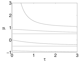
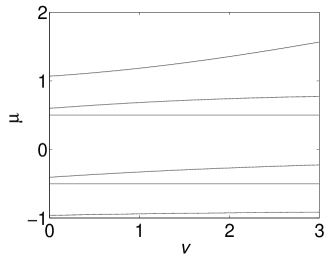
Figure 1: In both panels $U=\!0.05$ and $M=\!N=\!6$. Left panel: distribution of $\mu_{k}$ and $c_{k}=\cos(y_{k})$ as functions of $\tau$ for $V_{0}=\!0.4$. Right panel: distribution of $\mu_{k}$ and $c_{k}$ as functions of $v$ for $T=\!0.5$. SP energies are given by $-2\mu_{k}T$ and $-2Tc_{k}$.

The SI regime, where $U$ is large and $T/w<<M/4$, features SP energies $-\lambda_{k}$ that are small deviations from $-2T\cos({\bar{y}}_{k})$ “far” from $-2T\cos({y}_{k})$. In this case no doublet structure is found (see the left panel of figure 1 for small $\tau$) labels $y_{k}$, ${\bar{y}}_{k}$ of SP energies being uniformly distributed in interval $y\in[0,\pi]$. This case includes the situation where $U$ is weak or zero but well depth $V_{0}$ is large enough to sustain the boson localization on which our approximation relies.

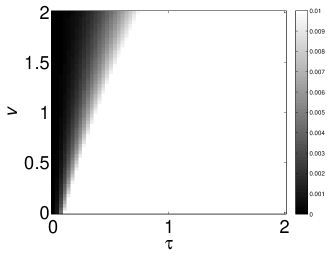
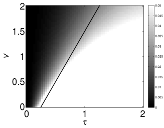
Figure 2: Relative error $|E_{0}-E_{\mathrm{gs}}|/E_{0}$ given in terms of the approximate ground-state energy $E_{\mathrm{gs}}$ and of its exact value $E_{0}$ for $M=\!N=\!6$. The grey scale describes the relative error whose maximum is 1 $\%$ (5 $\%$) in the left (right) panel.

In figure 2, the ground-state energy $E_{\mathrm{gs}}$ obtained from equation (18) is compared with the exact ground-state energy $E_{0}$, evaluated numerically, through the relative error $|E_{\mathrm{gs}}-E_{0}|/E_{0}$. In both panels, extended regions of plane $(\tau,v)$ appear to involve an almost negligible relative error. In the right panel, the straight line $v=2\tau-1/2$ roughly separates the region where the approximation of $E_{0}$ through $E_{\mathrm{gs}}$ is extremely good from the one where it becomes unsatisfactory. Such a separatrix can be obtained with a simple semiclassical argument: assume that operators $a_{i}$ and $a_{i}^{+}$ in Hamiltonian (3) are replaced by complex variables $z_{i}$ and $z_{i}^{*}$. Its semiclassical counterpart thus reads $H=-\sum_{i}U|z_{i}|^{4}/2-V_{0}|z_{0}|^{2}-T\sum_{i}(z^{*}_{i}z_{i+1}+z_{i}z^{*}_{i+1})$. The latter, depending on the value of $\tau$ and $v$, exhibits two possible ground-state configurations: $z_{0}=\sqrt{N}$, $z_{i}\simeq 0$ for $i\neq 0$ (solitonlike state) and $z_{i}\simeq\sqrt{N/M}$ (uniform state) giving

$$E^{\prime}_{0}=-N^{2}U\left(\frac{1}{2}+v\right),\,E^{\prime\prime}_{0}=-N^{2}U\left(\frac{1}{2M}+\frac{v}{M}+2\tau\right),$$

respectively. The situation where $E^{\prime}_{0}>E^{\prime\prime}_{0}$ and hence the ground state is uniform (SF regime) entails the inequality $v<2\tau-1/2$. Then the region where the approximation $E_{0}\simeq E_{\mathrm{gs}}$ is no longer satisfactory essentially identifies with the SF regime. Figure 3 describes the first five energy eigenvalues in the range $v\in[0,2]$ for $\tau=1/6$. Eigenvalues (18) well approximate qualitatively exact eigenvalues obtained numerically for $v>0.3$, consistent with figure 2. In particular, $E_{0}$ is almost indistiguishable from $E_{\mathrm{gs}}$.

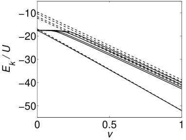
Figure 3: Dependence on $v=V_{0}/UN$ of the first five energy eigenvalues for $\tau=1/6$, $M=\!N=\!6$. Continuous lines describe exact eigenvalues obtained numerically, while dashed lines are obtained from formula (18).

To test our approximation scheme we further calculate the boson distribution in the ambient space corresponding to the ground state by exploiting the properties of SU($M$) coherent states [21]. To this end we reformulate operator $D^{+}_{0}$ in $|\mathrm{GS}\rangle$ in terms of space modes. This procedure, developed in appendix C, gives

$$n_{j}=\langle\mathrm{GS}|a^{+}_{j}a_{j}|\mathrm{GS}\rangle=N|\xi_{j}|^{2}=N\,\frac{2\,{\rm ch}^{2}[(M/2-j)y]}{M+{\rm sh}(My)\,{\rm coth}y}$$

obeying the normalization condition $\sum_{i}|\xi_{j}|^{2}=1$, together with the boson distribution $m_{k}=\langle\mathrm{GS}|b^{+}_{k}b_{k}|\mathrm{GS}\rangle$ $=N|x_{k}|^{2}$ among momentum modes where

$$|x_{k}|^{2}=\frac{2\,{\rm sh}^{2}(My/2)\,{\rm sh}^{2}y}{M+{\rm sh}(My)\,{\rm coth}y}\,\frac{1}{({\rm ch}y-c_{k})^{2}}\,.$$

In these two equations $e^{y}=(w/2T+\sqrt{1+w^{2}/4T^{2}})/2$ if $T/w<<M/4$, as stated by the second equation in formula (23). In the SI regime, where $UN>>T$, one has $e^{y}=w/2T>>1$ so that $n_{j}=N|\xi_{j}|^{2}\simeq N\exp(\,|2j-M|y-My)$. Note that index $j$ ranges in $[0,M-1]$ since $j=M$ is equivalent to $j=0$ in the ring geometry. Then the maximum occupation in the lattice is reached at $j=0$, where the boson-population peak is expected, while the minimum occupation is found at $j=M/2$. Figure 4 shows how $n_{j}$ is in an excellent agreement with the boson space distribution supplied by the exact (numeric) calculation of the ground state in regime $T/w<<M/4$. Figure 4 (right panel) confirms as well the validity of momentum-mode distribution $\langle m_{k}\rangle$ in the same regime.

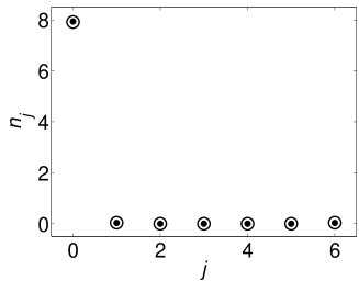
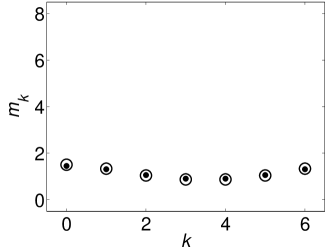
Figure 4: Space distribution $n_{j}=\langle a^{+}_{j}a_{j}\rangle$ (left panel) and momentum distribution $m_{k}=\langle b^{+}_{k}b_{k}\rangle$ (right panel) of bosons in the ground state for $T=\!0.5$, $V_{0}=\!0.1$, $U=\!1$, $M=\!7$, $N=\!8$. Symbols $\bigcirc$ and $\bullet$ describe the mode occupation relevant to the exact ground state and to its approximated form (19), respectively, showing an excellent agreement.

3 Spectrum of the SF regime

To determine the spectrum of model (3) within the SF regime we implement the standard Bogoliubov scheme involving the formulation of $H$ within momentum-mode picture. The full diagonal form of $H$ is achieved by means of a three-step procedure the first step of which consists in replacing $a_{j}$ with $a_{j}=\sum_{k}b_{k}\,{e^{i{\tilde{k}}j}}/{\sqrt{M}}$ and $b^{+}_{0}b_{0}$ with $b^{+}_{0}b_{0}=N-\sum_{k\neq 0}b^{+}_{k}b_{k}$. Hamiltonian (3) becomes

$$H\simeq H_{2}-V_{0}\,\sqrt{n}(B^{+}+B)-\Lambda$$ (26)

where $n=N/M$, the quadratic part of $H$ reads

$$H_{2}\simeq\sum_{k\neq 0}\Bigl{[}g_{k}b^{+}_{k}b_{k}-\frac{Un}{2}\,\left(b^{+}_{-k}b^{+}_{k}+b_{k}b_{-k}\right)\Bigr{]}-V_{0}B^{+}B$$

with $g_{k}={V_{0}}/{M}+e_{k}-Un$, $e_{k}=2T[1-\cos({\tilde{k}})]$, and

$$\Lambda=\frac{U}{2M}N(N-1)\,+\,2TN+nV_{0}\,,\quad B=\sum_{k\neq 0}\,\frac{b_{k}}{\sqrt{M}}\,.$$

The presence of the quadratic term $H_{2}$ in $H$ suggests that linear term $V_{0}\sqrt{n}(B^{+}+B)$ can be eliminated through the combined action of $k$-dependent displacement operators

$$T_{k}=e^{z_{k}b^{+}_{k}-z^{*}_{k}b_{k}}\,,\quad T_{k}b_{k}T^{+}_{k}=b_{k}-z_{k}\,.$$

As shown in appendix D, after implementing the unitary transformation $H\to{\cal H}=R^{+}HR$ with $R=\prod_{k\neq 0}T_{k}$, choice (41) of undetermined parameters $\eta_{k}$ provides

$${\cal H}=H_{2}-C\quad({\rm see\,formula}\,(\ref{qH}))$$

with $C=\Lambda+\Phi$ and $\Phi=nV_{0}/(1+S)$. The nice property of $\cal H$ is that it can be taken into a diagonal form by means of relatively simple calculations. Appendix D illustrates the second step of our procedure which consists in separating $H_{R}$ in two independent parts by exploiting again operators $f_{k}=(b_{k}-b_{-k})/{\sqrt{2}}$, $F_{k}=(b_{k}+b_{-k})/{\sqrt{2}}$ given in formula (7). One finds ${\cal H}={\cal H}_{f}+{\cal H}_{F}$ where

$${\cal H}_{f}=-C+\!\sum^{S}_{k=1}\Bigl{[}g_{k}f^{+}_{k}f_{k}+\frac{Un}{2}\Bigl{(}(f^{+}_{k})^{2}+f_{k}^{2}\Bigr{)}\Bigr{]}\,,$$

$${\cal H}_{F}=\!\sum^{K}_{k=1}\Bigl{[}g_{k}F^{+}_{k}F_{k}-\frac{Un}{2}\Bigl{(}(F^{+}_{k})^{2}+F_{k}^{2}\Bigr{)}\Bigr{]}-V_{0}B^{+}B\,,$$

where $B=\sum^{K}_{k=1}r_{k}F_{k}/{\sqrt{M}}$, $r_{k}$ is defined after equation (7), and parameters $S$ and $K$ have been defined in formulas (8) and (10). Hamiltonian ${\cal H}_{f}$ is easily diagonalized through the procedure described in [24], [25]. Since

$$J^{z}_{k}=\frac{2f^{+}_{k}f_{k}+1}{4},\,\,J^{x}_{k}=\frac{(f^{+}_{k})^{2}+f^{2}_{k}}{4},\,\,J^{y}_{k}=\frac{(f^{+}_{k})^{2}-f^{2}_{k}}{4i},$$

are, for each $k$, the generators of an algebra su(1,1) obeying commutators $[J^{x}_{k},J^{y}_{k}]=-2iJ^{z}_{k}$, $[J^{y}_{k},J^{z}_{k}]=2iJ^{x}_{k}$ and $[J^{z}_{k},J^{x}_{k}]=2iJ^{y}_{k}$, then the unitary transformation

$$D_{k}J^{z}_{k}D^{+}_{k}=J^{z}_{k}{\rm ch}\alpha_{k}+J^{x}_{k}{\rm sh}\alpha_{k}\,,\quad D_{k}=e^{-i\alpha_{k}J^{y}_{k}}\,,$$

allows one to diagonalize ${\cal H}_{f}$. We then rewrite ${\cal H}_{f}$ as

$${\cal H}_{f}={\sum}^{S}_{k=1}\Bigl{[}\,g_{k}(2J^{z}_{k}-1/2)+2UnJ^{x}_{k}\Bigr{]}-C\,.$$

whose diagonal form ${\rm H}_{f}$ is achieved by means of transformation $D=\Pi_{k}D_{k}$

$$D{\rm H}_{f}D^{+}=D\Bigl{[}\,{\sum}^{S}_{k=1}(2\nu_{k}J^{z}_{k}-{g_{k}}/{2})-C\Bigr{]}D^{+}={\cal H}_{f}\,,$$

if conditions $g_{k}=\nu_{k}{\rm ch}\alpha_{k}$ and $Un=\nu_{k}{\rm sh}\alpha_{k}$ are imposed. In ${\rm H}_{f}$ parameters $\nu_{k}$ read

$$\!\nu_{k}=\!\sqrt{g_{k}^{2}-U^{2}n^{2}}\!=\!\sqrt{\!\Bigl{(}\!{V_{0}}/{M}+e_{k}\!-\!Un\Bigr{)}^{2}-U^{2}n^{2}}$$ (27)

giving the energy eigenvalues relevant to ${\cal H}_{f}$

$$E_{f}({\vec{p}}\,)={\sum}^{S}_{k=1}\left[\,\nu_{k}(p_{k}+1/2)-{g_{k}}/{2}\right]-C$$

in the Fock-space basis formed by states $|{\vec{p}}\,\rangle=\prod^{S}_{k=1}|p_{k}\rangle$ where $f^{+}_{k}f_{k}|p_{k}\rangle=p_{k}|p_{k}\rangle$, $p_{k}=0,1,2...$ . The third and last step of the diagonalization process (see appendix D) concerns ${\cal H}_{F}$ which can be rewritten as

$${\cal H}_{F}=\!{\sum}^{K}_{k,h=1}G_{kh}F^{+}_{k}F_{h}-\frac{Un}{2}{\sum}^{K}_{k=1}\Bigl{(}F_{k}^{2}+\mathrm{H.C.}\Bigr{)}\,,$$

with $G_{kh}=g_{k}\delta_{kh}-V_{0}{r_{h}r_{k}}/{M}$. One can implement the same scheme applied for diagonalizing the component $H_{F}$ of $H_{w}$ in the SI regime. To this end we introduce new operators $C_{\ell}=\sum_{h}f_{h\ell}F_{h}$ and $C^{+}_{\ell}=\sum_{h}f_{h\ell}F^{+}_{h}$ such that $[C_{\ell},C^{+}_{m}]=\delta_{\ell m}$. Parameters $f_{h\ell}$ are undefined elements of an orthogonal matrix which can be exploited to take $G_{kh}$ into a diagonal form. Appendix D illustrates the calculations whereby the $C_{k}$-dependent final form

$${\cal H}_{C}={\sum}^{K}_{\ell=1}\theta_{\ell}C^{+}_{\ell}C_{\ell}-\frac{Un}{2}{\sum}^{K}_{k=1}\Bigl{(}(C^{+}_{k})^{2}+C_{k}^{2}\Bigr{)}$$

of Hamiltonian ${\cal H}_{C}$ is found together with $f_{h\ell}$ and $\theta_{\ell}$. The latter (see equations (47)) are given by

$$f_{h\ell}=-\frac{V_{0}}{M}\frac{r_{h}Y_{\ell}}{\theta_{\ell}-g_{h}}\,,\,\,1=-\frac{V_{0}}{M}\sum^{K}_{h=1}\frac{r^{2}_{h}}{\theta_{\ell}-g_{h}}\,,$$ (28)

where $Y_{\ell}=\sum^{K}_{k=1}r_{k}f_{k\ell}$ is determined in appendix D. Fortunately, Hamiltonian ${\cal H}_{C}$ exhibits the same algebraic structure of ${\cal H}_{f}$. Then, also in this case, its diagonal form ${\rm H}_{C}$ is connected to ${\cal H}_{C}$ by

$$W{\rm H}_{C}W^{+}=W\Bigl{[}\,{\sum}^{K}_{h=1}\left(2\eta_{h}V^{z}_{h}-{\theta_{h}}/{2}\right)\Bigr{]}W^{+}={\cal H}_{C}\,,$$

in which $W=\Pi_{k}W_{k}$ is a unitary transformation whose factors are defined as $W_{k}=\exp(i\beta_{k}V^{y}_{k})$. Similar to $J^{z}_{k}$, $J^{x}_{k}$ and $J^{y}_{k}$ operators $V^{z}_{k}$, $V^{x}_{k}$ and $V^{y}_{k}$ are, for each $k$, generators of an algebra su(1,1) written in terms of $C_{k}$ and $C^{+}_{k}$ instead of $f_{k}$, $f^{+}_{k}$. In particular, $V^{z}_{k}=(2C^{+}_{k}C_{k}+1)/4$. Conditions $\theta_{h}=\eta_{h}{\rm ch}\beta_{h}$ and $Un=\eta_{h}{\rm sh}\beta_{h}$ ensure that $W{\rm H}_{C}W^{+}={\cal H}_{C}$ and provide the definitions

$$\eta_{k}=\sqrt{\theta_{k}^{2}-U^{2}n^{2}}\,,\quad{\rm th}\beta_{k}={Un}/{\theta_{k}}\,.$$ (29)

Thanks to parameters $\eta_{h}$, we easily identify the energy eigenvalues relevant to ${\cal H}_{C}$ (and thus to ${\cal H}_{F}$)

$$E_{F}({\vec{q}}\,)={\sum}^{K}_{k=1}\left[\,\eta_{k}(q_{k}+1/2)-{\theta_{k}}/{2}\right]\,,\quad q_{k}=0,1,2...$$

in the Fock-space basis formed by states $|{\vec{q}}\,\rangle=\Pi_{k}|q_{k}\rangle$ where $C^{+}_{k}C_{k}|q_{k}\rangle=q_{k}|q_{k}\rangle$. Summarizing, the eigenvalues of total Hamiltonian ${\rm H}_{f}+{\rm H}_{C}$ are

$$E({\vec{p}},{\vec{q}}\,)=E_{F}({\vec{q}}\,)+E_{f}({\vec{p}}\,)\,,$$ (30)

corresponding to eigenvectors $|{\vec{p}},{\vec{q}}\rangle=\Pi^{S}_{k=1}|p_{k}\rangle\Pi^{K}_{h=1}|q_{h}\rangle$. Energies (30) provide as well the spectrum of Hamiltonian (26), whose eigenvalue problem is

$$H|E({\vec{p}},{\vec{q}}\,)\rangle=E({\vec{p}},{\vec{q}})|E({\vec{p}},{\vec{q}}\,)\rangle$$ (31)

where $|E({\vec{p}},{\vec{q}}\,)\rangle=RDW\,|{\vec{p}},{\vec{q}}\rangle$. This concludes the diagonalization process whose validity is supported by the fact that one has $\{\theta_{\ell}\}\equiv\{g_{k}\}$, $f_{k\ell}\equiv\delta_{k\ell}$, $C_{k}=F_{k}$ and $x_{k}=0$, for $V_{0}\to 0$. In this case the usual scenario relevant to the Bogoliubov scheme where $\eta_{k}\equiv\nu_{k}$ is recovered and no splitting effect, causing $\eta_{k}\neq\nu_{k}$, is observed.

3.1 Discussion

An important aspect of the diagonalization scheme leading to quasi-particle energies (27) and (29) concerns the range of parameters in which it should be valid. This is related to the conditions ensuring that quasi-particle energies are real and positive. The first condition is

$$g_{k}-Un=V_{0}/M+e_{k}-2Un>0\,,$$ (32)

which, being $g_{k}+Un=V_{0}/M+e_{k}>0$ for any $k$, implies that $g_{k}^{2}-U^{2}n^{2}>0$ in equation (27). The second one is

$$\theta_{k}+Un>0\,,\quad\theta_{k}-Un>0,$$ (33)

ensuring that $\theta_{k}^{2}-U^{2}n^{2}$ is positive in equation (29). By using parameters $\tau$ and $v$, inequality (32) reduces to

$${\tau}>{(1-v/2)}[\,2M\sin^{2}(\pi k/M)]^{-1}$$ (34)

which essentially reproduces the well-known condition establishing the parameter-$\tau$ interval in which the Bogoliubov approximation is valid. In the worst case ($k=1$) this inequality gives ${\tau}>(1-v/2){M}/{(2\pi^{2})}$ for large $M$. The novelty here is represented by factor $1-v/2$ showing that such an interval is enlarged because $v\neq 0$ due to the presence of local potential $V_{0}$.

Inequalities (33) involve a more complicated situation. Parameters $\theta_{\ell}$ are solutions of equation (28) which, being $g_{k}=V_{0}/M+2T(1-c_{k})-Un$ can be rewritten as

$$\frac{2TM}{V_{0}}=\!\sum_{k\neq 0}\!\left[\Bigl{(}1-\frac{UN-V_{0}}{2TM}-c_{k}\Bigr{)}-\mu\right]^{-1}\!={\cal F}(\mu)$$ (35)

with $\mu\equiv{\theta}/{2T}$ (we drop index $\ell$ of $\theta_{\ell}$ which is viewed as a continuous variable). In general, such an equation can be solved only numerically and no simple condition such as inequality (34) is available in this case.

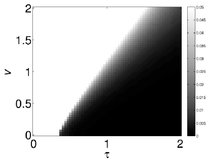
Figure 5: Relative error $|(E_{0}-E_{\mathrm{gs}})\,/\,E_{0}|$ given in terms of the approximate ground-state energy $E_{\mathrm{gs}}$ and of its exact value $E_{0}$ for $M=N=6$. The grey scale describes the relative error whose maximum is $5\%$.

The only exception is the regime ${2TM}/{V_{0}}>>1$ (when, for example, $V_{0}$ is perturbative and/or $M$ is large enough) in which approximate solutions can be found through an analytic approach (see Appendix E). In this regime the number of solutions is expected to coincide with the number $K$ of the asymptotes characterizing ${\cal F}(\mu)$ so that the quasi-particle energy spectrum exhibits an evident doublet structure being $\eta_{k}\simeq\nu_{k}$.

After setting $\mu=V_{0}/(2TM)-Un/(2T)+1-\cos y$, approximate solutions of $2TM/V_{0}={\cal F}(\mu)$ are found by substituting $y=y_{k}+\xi_{k}$ in its trigonometric version (49). The Taylor expansion of the latter to the second order in $\xi_{k}$ yields equation (50) whose solutions (51), at fixed $M$ and with $t=8T/(MV_{0})$ sufficiently large, reduce to $\xi_{k}=-{8}/{(tM^{2}s_{k})}$ entailing

$$\theta_{k}=2T\mu_{k}=\frac{V_{0}}{M}-Un+2T(1-\cos(y_{k}+\xi_{k}))\simeq g_{k}-\frac{2V_{0}}{M}.$$

These results show that the two conditions (33), now expressed as $g_{k}-2V_{0}/M>\pm Un$ and therefore as

$$4\tau M\sin^{2}(\pi k/M)>v\,,\quad 4\tau M\sin^{2}(\pi k/M)-2>v,$$

can be fulfilled for large enough $\tau$ and sufficiently small $v$ in plane $v$-$\tau$ even in the most restrictive case $k=1$. Of course these inequalities supply a limited information on the range of validity of our scheme since they have been obtained in the limiting case $t>>1$. A complete information is provided by inequalities (33) only through a systematic numerical study of solutions $\theta_{\ell}$ when the model parameters are varied. This analysis is beyond the scope of this work.

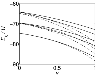
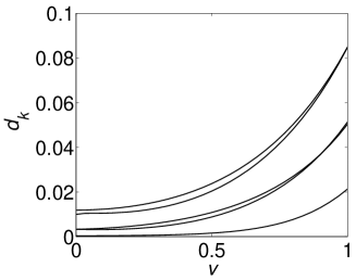
Figure 6: Left panel: dependence on $v$ of the first five energy eigenvalues for $\tau=1$, $M=\!N=\!6$. Continuous lines describe exact eigenvalues denoted by $E_{k}$ ($0\leq k\leq 4$) obtained numerically, while dashed lines describe eigenvalues $E^{\mathrm{ap}}_{k}$ obtained from formula (30). Right panel: $d_{k}=|(E_{k}-E^{\mathrm{ap}}_{k})/E_{k}|$

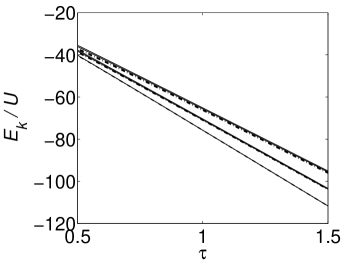
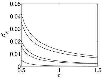
Figure 7: Left panel: dependence on $\tau$ of the first five energy eigenvalues for $v=1/6$, $M=\!N=\!6$. Continuous lines describing $E_{k}$ and dashed lines describing $E^{\mathrm{ap}}_{k}$ have the same meaning as in figure 6. Right panel: $d_{k}=|(E_{k}-E^{\mathrm{ap}}_{k})/E_{k}|$

Here we limit our attention to some specific cases. In Figure 5, the ground-state energy $E_{\mathrm{gs}}$, given by equation (30) with $p_{k}\,=\,q_{h}\,=\,0$ for all $k$ and $h$, is compared with the exact ground-state energy $E_{0}$, evaluated numerically: in the figure the relative error $|(E_{\mathrm{gs}}\,-\,E_{0})\,/\,E_{0}|$ is plotted as a function of $v$ and $\tau$. Also in this case, extended regions of the $(\tau;\,v)$ plane show an almost negligible relative error. In particular, at increasing values of $\tau$ one can see that the results provided by the Bogoliubov approximation become more precise, while the rise in $v$ implies a fast decrease in the effectiveness of the approximation in the prediction of the ground-state energy.

The scenario outlined in the previous paragraph is further confirmed by the numerical calculations of the first low-energy excited levels, illustrated in figure 6 and 7. In figure 6, where $\tau=1$ while $v$ varies, the first five energy eigenvalues $E_{k}$, $k\in[0,4]$ ($E_{0}$ corresponds to the ground state) obtained numerically can be compared with energies $E^{\mathrm{ap}}_{k}$ given by formula (30) within the Bogoliubov approximation. The agreement is, in general, extremely good for $v<0.5$, and becomes excellent in the case of the ground state, as shown by the relative error $d_{k}$ in the right panel of figure 6. Figure 7, where $v=1/6$ while $\tau$ varies, shows that the agreement between $E^{\mathrm{ap}}_{k}$ and $E_{k}$ is excellent for any value of $\tau>0.5$. For $\tau<0.5$ (this case is not shown) the deviation of $E^{\mathrm{ap}}_{k}$ from $E_{k}$ becomes significant.

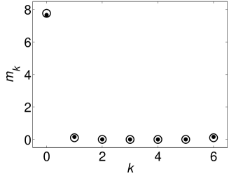
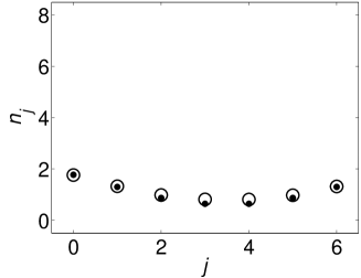
Figure 8: Momentum distribution $m_{k}$ (left panel) and space distribution $n_{j}$ (right panel) of bosons in the ground state for $T=\!1$, $V_{0}=\!0.2$, $U=\!0.2$, $M=\!7$, $N=\!8$. Symbols $\bigcirc$ and $\bullet$ have the same meaning as in figure 4 and show an excellent agreement between the distributions relevant to the exact and the approximate ground state.

As in the case of the SI-regime spectrum, we conclude by reconstructing the boson distribution both among space modes and among momentum modes through the formulas $n_{i}=\langle\mathrm{GS}|a^{+}_{i}a_{i}|\mathrm{GS}\rangle$ and $m_{k}=\langle\mathrm{GS}|b^{+}_{k}b_{k}|\mathrm{GS}\rangle$ where $|\mathrm{GS}\rangle$ now represents the approximate SF ground state. Observing that $|\mathrm{GS}\rangle=|E({\vec{p}},{\vec{q}})\rangle=RDW\,|{\vec{p}},{\vec{q}}\rangle$ with ${\vec{p}}=0={\vec{q}}$, it is advantageous to define operators ${\cal B}_{k}=(RDW)^{+}b_{k}RDW$ whose explicit expression is

$${\cal B}_{k}=x_{k}+\frac{1}{2}D_{k}^{+}f_{k}D_{k}+\frac{1}{2}{\sum}^{K}_{\ell=1}f_{k\ell}W_{\ell}^{+}C_{\ell}W_{\ell}\,.$$ (36)

In this formula $D_{k}^{+}f_{k}D_{k}=f_{k}{\rm ch}(\alpha_{k}/2)-f^{+}_{k}{\rm sh}(\alpha_{k}/2)$ while $W_{k}^{+}C_{k}W_{k}=C_{k}{\rm ch}(\beta_{k}/2)+C^{+}_{k}{\rm sh}(\beta_{k}/2)$. The calculation of $m_{k}$ remarkably simplifies since $\langle\mathrm{GS}|b^{+}_{k}b_{k}|\mathrm{GS}\rangle=\langle 0,0|{\cal B}^{+}_{k}{\cal B}_{k}|0,0\rangle$ where the simple ground state $|0,0\rangle$ of diagonal Hamiltonian ${\rm H}_{f}+{\rm H}_{C}$ can be used. The resulting momentum mode distribution reads

$$m_{k}=\langle b^{+}_{k}b_{k}\rangle=x^{2}_{k}+\frac{{\rm sh}^{2}(\alpha_{k}/2)}{2}+\frac{1}{2}{\sum}^{K}_{h=1}f^{2}_{kh}{\rm sh}^{2}(\beta_{h}/2)$$

while the ground-state distribution among space modes $n_{\ell}=\langle a^{+}_{\ell}a_{\ell}\rangle=\sum_{k}\sum_{q}\exp[i({\tilde{k}}-{\tilde{q}})\ell]\langle b^{+}_{q}b_{k}\rangle/M$ is achieved by resorting again to formula (36) to calculate $\langle b^{+}_{q}b_{k}\rangle$. Figure 8 shows that essentially no difference is visible between the values of $m_{k}$ and $n_{i}$ obtained with a ground state determined numerically and those supplied by our approximation scheme. We note that the choice of parameters in figure 8 entails that $\tau=0.625=5v$ and, in particular, $2TM/V_{0}=70>>1$. Then the conditions for which solutions $\theta_{k}\simeq g_{k}$ in equation (35) are satisfied. In figure 9, where condition $2TM/V_{0}>>1$ is weakened ($2TM/V_{0}=22.4$), distributions based on $|\mathrm{GS}\rangle$ show some deviations from those based on the exact ground state. Their agreement however is still very satisfactory. In both cases the approximation $\theta_{k}\simeq g_{k}-2V_{0}/M$ cannot be used since the more restrictive condition $t>>1$ is never reached.

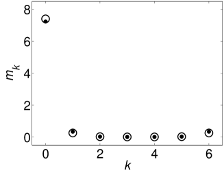
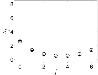
Figure 9: Momentum distribution $m_{k}$ (left panel) and space distribution $n_{j}$ (right panel) of bosons in the ground state for $T=\!1.6$, $V_{0}=\!1$, $U=\!0.1$, $M=\!7$, $N=\!8$. Symbols $\bigcirc$ and $\bullet$ have the same meaning as in figure 4 and show an satisfactory agreement between the distributions relevant to the exact and the approximate ground state.

4 Conclusions

In this paper we have analysed the properties of attractive bosons trapped in a 1D optical lattice in the presence of a localized attractive potential. The two particular regimes that we have considered (the SI and the SF one) allow a completely analytical approach by means of a Bogoliubov-type approximation.

In section 2 we observed that in the SI regime the localization of bosons, enhanced by the presence of a single attractive potential well, allows one to obtain the approximate Hamiltonian (6). The diagonalization of the latter gives an excellent description of the main properties of the ground-state and of the low-excited states, in terms of energy and mean occupation number in the ambient and momentum space. The comparison between analytical and numerical results (the latter are necessary to compute the exact spectrum of Hamiltonian (3)) allows one to identify the region in the parameter space in which the SI hypothesis is satisfied and thus the approximation is valid.

In addition, the opposite SF regime has been studied in section 3 by applying a Bogoliubov-type treatment justified by the hypothesis of localization in the momentum space. The simplification introduced has enabled us to compute the spectrum and the mean occupation number of particles in the ambient and momentum space. Also in this case, the support of numerical results makes it possible to show for which values of the parameters the Bogoliubov approximation is actually effective.

The possibility to study our model Hamiltonian in a fully analytical manner is obviously due to the simple shape of potential $V$ which just reduces to a single localized potential. However, despite its simplicity, this model represents an instructive intermediate step toward more structured systems such as lattices with several defects (local potentials with perturbative depths) or, more in general, to lattices with many local potentials possibly characterized by random depths: even if the approach to such systems will be mainly numeric, we expect that the methodology and the analytical results contained in this paper still represent useful tools. We expects as well that our approach may be fruitfully applied to other condensed-matter models. The scheme applied to model (26) in section 2, for example, should be applicable in the diagonalization of the polaron-like Hamiltonian of mixtures with two atomic species [26]. Also, simple heuristic calculations show that the repulsive version ($U\to-U$) of model (3) could be studied through the scheme of section 2 for $V_{0}>2T+UN/2$. Finally, the knowledge of low-energy states achieved in the attractive case is necessary to investigate the model when the local potential is time dependent. The study of this case is in progress and will be discussed elsewhere.

At the experimental level, the lattice with a single localized potential could be more than a simple but interesting toy model since it certainly represents the simplest way to break the translational symmetry of the BH Hamiltonian and thus to make appear the spatial localization, when present. In this respect the realization of toroidal traps [27] with a persistent flow is encouraging. This system has raised a lot of interest owing to the possibility to create a bosonic Josephson junction by intersecting the toroidal domain with a transverse laser beam to generate a potential barrier. In our periodic-lattice model a possible experimental realization of the local potential could be achieved by using a red detuned laser beam.

Appendix A Number of solutions of equation (20)

The two parametrizations $\mu=\,{\rm ch}y$ and $\mu=\,\cos y$, allow one to rewrite equation (20) as

$${\sum}^{M-1}_{k=0}\frac{1}{{\rm ch}y-c_{k}}=\frac{M\,{\rm sh}(My)}{{\rm sh}y\,[{\rm ch}(My)-1]}\,,$$ (37)

$${\sum}^{M-1}_{k=0}\frac{1}{\cos y-c_{k}}=\frac{M\,\sin(My)}{\sin y\,[\cos(My)-1]}\,,$$ (38)

giving equations (21) and (22). Their extremely simple form is particularly useful to find single-particle energies $\lambda_{k}$ both numerically and analytically. Nevertheless, the series-like version (20) of such equations better elucidates the dependence of the effective number of solutions $\lambda_{k}$ from parameter $M$. By assuming, in equation (20), the equivalent ranges $k\,\in[-\frac{M}{2}+1,\,\frac{M}{2}]$, for $M=2p$, and $k\,\in[-\frac{M-1}{2},\,\frac{M-1}{2}]$, for $M=\,2p+1$, one finds

$$\frac{2TM}{w}=\frac{1}{\cos y-1}+\frac{1}{\cos y+1}+{\sum}^{p-1}_{k=1}\frac{2}{\cos y-c_{k}}\,,$$

(remind that $c_{k}=\cos(2\pi k/M)$) for $M=\,2p$ and

$$\frac{2TM}{w}\,=\frac{1}{\cos y-1}+{\sum}^{p}_{k=1}\frac{2}{\cos y-c_{k}}\,,$$

for $M=\,2p+1$. It is thus evident how in $\lambda=2T\,\cos y$ the values of $y$ solving such equations are in one-to-one correspondence with critical values $y_{k}=2\pi k/M>0$ and that for sufficiently large $TM/w$ one has $y\simeq y_{k}$. In particular, for $M=2p$, the number of different eigenvalues is $p={M}/{2}$, while $p=(M-1)/{2}$ is found for $M=2p+1$. In both cases term $1/(\cos y-1)$ occurring in the preceding formulas does not generate any solution in that it tends to $-\infty$ while ${2TM}/{w}$ is positive. Including the isolated solution given by equation (21), the solution number is ${M}/{2}+1$ for $M=2p$ and $(M+1)/{2}$ for $M=2p+1$.

Appendix B Approximate solutions of equation (22)

For $2T/w>>M/2$, function $z(y)=\frac{2T}{w}\,\sin(y)$ intercepts $z(y)={\rm cot}(My/2)$ in the proximity of its asymptotes placed at $y=y_{k}=2\pi k/M$ in the interval $[0,\pi]$. Substituting $y=y_{k}+\epsilon_{k}$ with $|\epsilon_{k}|<<y_{k}$ in equation (22) gives $({2T}/{w})\,\sin(y_{k}+\epsilon_{k})=-{\rm ctg}(M\epsilon_{k}/2)$, which, with the further assumption $M\epsilon_{k}<<1$, becomes, to the second order in $M\epsilon_{k}$,

$$\left(\eta c_{k}-1\right)\,\epsilon_{k}^{2}+\eta s_{k}\,\epsilon_{k}\,+{8}/{M^{2}}\,=0\,,\quad\eta={8T}/({wM})\,,$$

with $s_{k}=\sin(2\pi k/M)$ and, as usual, $c_{k}=\cos(2\pi k/M)$. The ensuing solutions are

$$\epsilon_{k}=\frac{1}{2(\eta c_{k}-1)}\left[-\eta s_{k}\pm{\sqrt{\eta^{2}s^{2}_{k}-{32}(\eta c_{k}-1)/{M^{2}}}}\right]$$

where one should remind that cases $k=0$ and (in even-$M$ case) $k=M/2$ are excluded. These solutions are well defined for $\eta>>1$, a condition that perfectly matches initial assumption $2T/w>>M/2$. For large $\eta$, one obtains $\epsilon_{k}\simeq-8/(\eta M^{2}s_{k})$ giving the approximate solutions

$${\lambda_{k}}/{(2T)}=\cos(y_{k}+\epsilon_{k})\simeq\,\cos(y_{k})\,+{8}/{(\eta M^{2})}\,,$$

where $\cos(y_{k}+\epsilon_{k})\simeq\cos(y_{k})\,+|\epsilon_{k}|\,\sin(y_{k})$ has been used. Notice that, at least to the first order in $1/\eta$, energies $\lambda_{k}$ simply represent a shift from values $\cos(y_{k})$. In order to satisfy condition $\eta=8T/(wM)>>1$, the potential-well depth $w$ (the hopping amplitude $T$) must be much smaller (larger) than $T$ ($w$). This request, however, is not matched in the SI regime since $T/UN<1$ and the effective depth $w=UN+v_{0}\simeq UN$ due to $v_{0}<<UN$. Then the opposite regime described by the inequality $1>>8T/(wM)$ must be considered.

This circumstance suggests to develop a different approximation scheme. Owing to $1>>8T/(wM)$, function $({2T}/{w})\sin y$ in equation (22) ends up intercept ${\rm ctg}(My/2)$ close to the zeros thereof. As a consequence $y={\bar{y}}_{k}+\epsilon_{k}$, with ${\bar{y}}_{k}=y_{k}+\pi/M$, where, locally, ${\rm ctg}(My/2)\simeq-{M}(y-{\bar{y}}_{k})/2$. Then, by considering only first-order terms, equation (22) becomes $({2T}/{w})\sin({\bar{y}}_{k}+\epsilon_{k})\simeq{M}\epsilon_{k}/{2}$ giving in turn $\epsilon_{k}\simeq({4T}/{wM})\sin({\bar{y}}_{k})$ and

$${\lambda_{k}}/({2T})=\cos({\bar{y}}_{k}+\epsilon_{k})\simeq\,\cos({\bar{y}}_{k})\,+{4T}\,\sin^{2}({\bar{y}}_{k})/({wM})\,,$$

due to approximation $\cos({\bar{y}}_{k}+\epsilon_{k})\simeq\cos({\bar{y}}_{k})\,+\epsilon_{k}\,\sin({\bar{y}}_{k})$.

Appendix C Ground-state boson distribution

The boson distrubution in the ambient space involved by state (19) is obtained by calculating $\langle\mathrm{GS}|a^{+}_{j}a_{j}|\mathrm{GS}\rangle$. To this end it is useful to reformulate the ground state in terms of spacelike boson operators. From equations (13) and the fact that $F^{+}_{0}=b^{+}_{0}$, $F^{+}_{k}=(b^{+}_{k}+b^{+}_{-k})/\sqrt{2}$ one has

$$D^{+}_{0}=\sum^{K}_{k=0}{B}_{0k}\,F^{+}_{k}=\sum^{K}_{k=0}\frac{wr_{k}}{M}\,\frac{A(0)}{\lambda_{0}-2Tc_{k}}\,F^{+}_{k}=\sum^{M-1}_{k=0}x_{k}\,b^{+}_{k}$$

with $x_{k}={wA(0)}/{[M(\lambda_{0}-2Tc_{k})]}$. Then ground state (19) reduces to $|\mathrm{GS}\rangle=\left(\sum^{M-1}_{k=0}x_{k}\,b^{+}_{k}\right)^{N}\,|0\rangle/{\sqrt{N!}}$. The latter is a SU($M$) coherent state with the normalization condition $\sum_{k}|x_{k}|^{2}=1$ (this exactly matches equation (14)) and the properties that the momentum-mode and space-mode boson distributions are given by [21]

$$\langle\mathrm{GS}|b^{+}_{q}b_{q}|\mathrm{GS}\rangle=N|x_{q}|^{2}\,,\quad\langle\mathrm{GS}|a^{+}_{j}a_{j}|\mathrm{GS}\rangle=N|\xi_{j}|^{2}$$

respectively, being

$$D^{+}_{0}=\sum^{M-1}_{k=0}x_{k}\,b^{+}_{k}=\sum^{M-1}_{\ell=0}\xi_{\ell}\,a^{+}_{\ell}\,,\quad\xi_{\ell}=\sum^{M-1}_{k=0}x_{k}\,{e^{i{\tilde{k}}\ell}}/{\sqrt{M}}\,,$$

owing to definitions (5). After setting $\lambda_{0}=2T{\rm ch}y$, the series in $\xi_{\ell}$ can be computed explicitly giving

$$\xi_{j}=\frac{wA(0)}{2TM^{3/2}}\sum^{M-1}_{k=0}\,\frac{e^{i{\tilde{k}}j}}{{\rm ch}y-c_{k}}=\frac{wA(0)}{2TM^{3/2}}\,\frac{{\rm ch}[(M/2-j)y]}{{\rm sh}y\,{\rm sh}(My/2)}\,.$$

Equation (14) provides $A(0)$

$$\frac{1}{|A(0)|^{2}}=\sum^{K}_{k=0}\frac{w^{2}r_{k}^{2}/M^{2}}{(\lambda_{0}-2Tc_{k})^{2}}=\frac{w^{2}}{(2TM)^{2}}\sum^{M-1}_{k=0}\frac{1}{({\rm ch}y-c_{k})^{2}}$$

$$=\frac{w^{2}}{(2TM)^{2}}\frac{M+{\rm sh}(My)\,{\rm coth}y}{2\,{\rm sh}^{2}(My/2)\,{\rm sh}^{2}y}\,.$$

Then, the boson distribution in the ambient space reads

$$\langle\mathrm{GS}|a^{+}_{j}a_{j}|\mathrm{GS}\rangle=N|\xi_{j}|^{2}=2N\,\frac{{\rm ch}^{2}[(M/2-j)y]}{M+{\rm sh}(My)\,{\rm coth}y}$$

Appendix D Diagonalization of SF Hamiltonian

The action of $R=\prod_{k\neq 0}T_{k}$ on Hamiltonian (26) entails that $b_{k}^{+}\to b_{k}^{+}+z^{*}_{k}$ and $b_{k}\to b_{k}+z_{k}$. The new Hamiltonian contains a linear term ${\cal L}$ depending on parameters $z^{*}_{k}$ and $z_{k}$ which can be removed by exploiting the arbitrariness of $z^{*}_{k}$ and $z_{k}$. After some algebra, the new Hamiltonian is found to have the form

$${\cal H}=R^{+}HR=-\Lambda+1/2\,\sum^{\prime}_{k}g_{k}\bigl{(}n_{k}+n_{-k}\bigr{)}$$

$$-1/2\,{\sum}^{\prime}_{k}Un\,\left(b^{+}_{-k}b^{+}_{k}+\,b_{k}b_{-k}\right)-V_{0}B^{+}B+{\cal L}+\Phi$$

with ${\sum}^{\prime}_{k}={\sum}_{k\neq 0}$, where ${\cal L}$ is defined as

$${\cal L}={\sum}^{\prime}_{k}\Bigl{[}\,g_{k}\Bigl{(}z_{k}b_{k}^{+}+z^{*}_{k}b_{k}\Bigr{)}-Un\left(z^{*}_{-k}b^{+}_{k}+\,b_{k}z_{-k}\right)\Bigr{]}$$

$$-V_{0}\,\sqrt{n}(B^{+}+B)-\frac{V_{0}}{\sqrt{M}}\Bigl{(}B{\sum}^{\prime}_{k}z^{*}_{k}+B^{+}{\sum}^{\prime}_{k}z_{k}\Bigr{)}\,,$$

and

$$\Phi={\sum}^{\prime}_{k}\frac{g_{k}}{2}\Bigl{(}|z_{k}|^{2}+|z_{-k}|^{2}\Bigr{)}-{\sum}^{\prime}_{k}\frac{Un}{2}\,\left(z^{*}_{-k}z^{*}_{k}+\,z_{k}z_{-k}\right)$$

$$-({V_{0}}/{M}){\sum}^{\prime}_{k}{\sum}^{\prime}_{h}\,z^{*}_{h}z_{k}-{V_{0}}{\sqrt{n/M}}\,{\sum}^{\prime}_{k}(z^{*}_{k}+z_{k})\,.$$

${\cal L}$ vanishes if the following equations are satisfied

$$V_{0}\sqrt{n/M}=g_{k}z_{k}-Unz^{*}_{-k}-\frac{V_{0}}{M}{\sum}_{k\neq 0}z_{k}\,,$$ (39)

Exploiting the fact that $g_{k}=g_{-k}$ one can show that $z_{k}\equiv z_{-k}=x_{k}$. The new equation for $x_{k}$’s reads $V_{0}\sqrt{n/M}=(g_{k}-Un)x_{k}-XV_{0}/{M}$, with $X=\sum_{k\neq 0}x_{k}$, giving

$$x_{k}=\frac{V_{0}}{g_{k}-Un}\,\left(\frac{\sqrt{n}}{\sqrt{M}}+\frac{X}{M}\right)=-\frac{V_{0}(X+{\sqrt{N}})}{UN-Mg_{k}}\,.$$ (40)

Summing on index $k$ on both the left and right-hand side of equation (40) provides $X=-{S{\sqrt{N}}}/{(1+S)}$ in which $S=\sum_{k\neq 0}{V_{0}}/{(UN-Mg_{k})}$, and

$$x_{k}=-\frac{V_{0}{\sqrt{N}}}{(UN-Mg_{k})(1+S)}$$ (41)

determining parameters $x_{k}$. As a consequence, one can simplify the scalar terms $\Phi$ depending on $z_{k}$’s in $\cal H$ finding $\Phi=NV_{0}/[M(1+S)]$. The Hamiltonian becomes

$${\cal H}=\!\sum_{k\neq 0}\!\left(g_{k}n_{k}-\frac{Un}{2}(b^{+}_{-k}b^{+}_{k}+\,b_{k}b_{-k})\right)-V_{0}B^{+}\!B-C$$ (42)

with $C=\Lambda+\Phi$, and thus

$${\cal H}=\!\sum_{h,k\neq 0}\Bigl{(}g_{k}\delta_{kh}-\frac{V_{0}}{M}\Bigr{)}b^{+}_{h}b_{k}-\frac{Un}{2}\sum_{k\neq 0}(b^{+}_{-k}b^{+}_{k}+\mathrm{H.C.})-C.$$

The latter can be separated in two independent parts by exploiting operators $f_{k}$ and $F_{k}$ (see equation (7)) such that $F_{0}=b_{0}$ and $f_{0}=0$ (remind that, if $M$ is even, operator $F_{M/2}=b_{M/2}$ must be considered while $f_{M/2}=0$). By observing that $b^{+}_{-k}b^{+}_{k}+b_{-k}b_{k}=(F^{+}_{k})^{2}+F_{k}^{2}-(f^{+}_{k})^{2}-f_{k}^{2}$ and $n_{k}+n_{-k}=F^{+}_{k}F_{k}+f^{+}_{k}f_{k}$, Hamiltonian ${\cal H}$ reduces to ${\cal H}={\cal H}_{f}+{\cal H}_{F}$ where

$${\cal H}_{f}=\!\sum^{S}_{k=1}\Bigl{[}g_{k}f^{+}_{k}f_{k}+Un\Bigl{(}(f^{+}_{k})^{2}+f_{k}^{2}\Bigl{)}\Bigl{]}-C\,,$$ (43)

$${\cal H}_{F}=\!\sum^{K}_{k=1}\Bigl{[}\,g_{k}F^{+}_{k}F_{k}-Un\Bigl{(}F_{k}^{2}+\mathrm{H.C.}\Bigr{)}\Bigr{]}-V_{0}B^{+}B.$$ (44)

In operator $B=\sum^{K}_{k=1}r_{k}F_{k}/{\sqrt{M}}$, apart from $r^{2}_{M/2}=1$ when $M$ is even, $r^{2}_{k}=2$. The ranges of $S$ and $K$ are defined in equations (8) and (10), respectively.

The third and last step for diagonalizing ${\cal H}$ concerns ${\cal H}_{F}$ which, after setting $G_{kh}=g_{k}\delta_{kh}-V_{0}{r_{k}r_{h}}/{M}$, reads

$${\cal H}_{F}={\sum}^{K}_{k,h=1}G_{kh}F^{+}_{k}F_{h}-\frac{Un}{2}{\sum}^{K}_{k=1}\Bigl{(}F_{k}^{2}+\mathrm{H.C.}\Bigr{)}\,.$$

To get the diagonal form of ${\cal H}_{F}$ we define new operators $C_{\ell}=\sum_{h}f_{h\ell}F_{h}$ and $C^{+}_{\ell}=\sum_{h}f_{h\ell}F^{+}_{h}$ where $f_{h\ell}$ are undetermined elements of an orthogonal matrix whose arbitrariness can be exploited to diagonalize matrix $G_{kh}$. We remind that the orthogonal-matrix properties

$${\sum}^{K}_{h=1}f_{h\ell}f_{hm}=\delta_{\ell m}\,,\,\,{\sum}^{K}_{k=1}f_{\ell k}f_{mk}=\delta_{\ell m}\,,$$ (45)

are equivalent to the commutation relations $[C_{\ell},C^{+}_{m}]=\delta_{\ell m}$ and $[F_{\ell},F^{+}_{m}]=\delta_{\ell m}$. Imposing that

$${\sum}^{K}_{k,h=1}G_{kh}F^{+}_{k}F_{h}={\sum}^{K}_{\ell=1}\theta_{\ell}C^{+}_{\ell}C_{\ell}$$

yields the condition $\theta_{\ell}f_{h\ell}=g_{h}f_{h\ell}-({V_{0}}/{M})r_{h}Y_{\ell}$, in which $Y_{\ell}=\sum^{K}_{k=1}r_{k}f_{k\ell}$, giving in turn the two equations

$$f_{h\ell}=-\frac{V_{0}}{M}\frac{r_{h}Y_{\ell}}{\theta_{\ell}-g_{h}}\,,\,\,1=-\frac{V_{0}}{M}\sum^{K}_{h=1}\frac{r^{2}_{h}}{\theta_{\ell}-g_{h}}\,.$$ (46)

The second equation easily follows from the first one. Owing to $g_{h}=g_{-h}$, equation (46) can be written in the more general form

$$1=-\frac{V_{0}}{M}{\sum}_{h\neq 0}\,\frac{1}{\theta_{\ell}-g_{h}}\,.$$ (47)

Moreover, the calculation of $\sum_{h}f_{hm}f_{h\ell}$ for $m=\ell$ gives $|Y_{\ell}|^{-2}=({V_{0}^{2}}/{M^{2}})\sum_{h}\,{r_{h}^{2}}/{(\theta_{\ell}-g_{h})^{2}}$ thus fixing $Y_{\ell}$. The final form of Hamiltonian ${\cal H}_{F}$ is found to be

$${\cal H}_{C}={\sum}^{K}_{\ell=1}\Bigl{[}\theta_{\ell}C^{+}_{\ell}C_{\ell}-\frac{Un}{2}\Bigl{(}(C^{+}_{\ell})^{2}+C_{\ell}^{2}\Bigr{)}\Bigr{]}$$ (48)

thanks to the identity $\sum_{\ell}C_{\ell}^{2}=\sum_{h,k}\sum_{\ell}f_{h\ell}f_{k\ell}F_{h}F_{k}=\sum_{\ell}F_{k}^{2}$ ($\Rightarrow$ $\sum_{\ell}(C^{+}_{\ell})^{2}=\sum_{\ell}(F^{+}_{\ell})^{2}$). This can be easily proven by means of equations (45).

Appendix E Calculation of parameters $\theta_{\ell}$

Since $g_{k}=V_{0}/M+2T(1-c_{k})-Un$ equation (28) (equivalent to (47)) takes the form ${\cal F}(\mu)={2TM}/{V_{0}}$ described by equation (35) where

$${\cal F}(\mu)=-\sum_{k\neq 0}\left[\,\mu-\left(1-\frac{UN-V_{0}}{2TM}-c_{k}\right)\right]^{-1}$$

with $\mu\equiv{\theta}/{2T}$. In the regime ${2TM}/{V_{0}}>>1$ one expects that the solutions of such an equation are values of $\theta$ very close to the asymptote positions $g_{k}$. This suggests in turn to represent $\mu$ as $\mu=V_{0}/(2TM)-Un/(2T)+1-\cos y$ leading to equation

$$\frac{2TM}{V_{0}}=\frac{1}{1-\cos y}+{\sum}_{k}\,\frac{1}{\cos y-c_{k}}\,.$$

Equation (28) clearly shows how the asymptotes of ${\cal F}(\mu)$ are $K$ and thus one expects to find $K$ solutions. Thanks to equation (38), the latter becomes

$$({2TM}/{V_{0}})\sin y\,={\rm ctg}(y/2)-M\,{\rm ctg}(My/2)\,.$$ (49)

Approximated solutions are found by replacing $y=y_{k}+\xi_{k}$ in the latter formula and using the Taylor expansion to the second order in $\xi_{k}$. This supplies the equation

$$\frac{2TM}{V_{0}}(s_{k}+c_{k}\xi_{k})\xi_{k}=\frac{\xi_{k}s_{k}-\xi^{2}_{k}}{1-c_{k}}-2+\frac{M^{2}}{4}\xi^{2}_{k}\,.$$

($s_{k}=\sin y_{k}$, $c_{k}=\cos y_{k}$) giving in turn

$$(tc_{k}-1+\rho_{k})\xi^{2}_{k}+(t-\rho_{k})s_{k}\xi_{k}+{8}/{M^{2}}=0\,.$$ (50)

with $t={8T}/{MV_{0}}$ and $\rho_{k}={4}/[M^{2}(1-c_{k})]$. At fixed $M$ with $T/V_{0}$ sufficiently large, $\rho_{k}$ appears to be negligible with respect to $t$ for each $k\in[1,K]$. Then the solutions are found to be

$$\xi_{k}=\frac{1}{2(tc_{k}-1+\rho_{k})}\Bigl{[}-(t-\rho_{k})s_{k}\pm{\cal R}_{k}(t,M)\,\Bigr{]}$$ (51)

where ${\cal R}_{k}(t,M)\equiv\sqrt{(t-\rho_{k})^{2}s^{2}_{k}-32(tc_{k}-1+\rho_{k})/M^{2}}$.

References

References

- [1] Jack M W, and Yamashita M 2005 Phys. Rev. A 71 023610
- [2] Buonsante P, Penna V, and Vezzani A 2005 Phys. Rev. A 72 043620
- [3] Buonsante P, Kevrekidis P, Penna V, and Vezzani A 2006 J. Phys. B: At. Mol. Opt. Phys. 39 S77
- [4] Buonsante P, Kevrekidis P, Penna V, and Vezzani A 2007 Phys. Rev. E 75 016212
- [5] Oelkers N, and Links J 2007 Phys. Rev. B 75 115119
- [6] Ho T-L, and Ciobanu C V, 2001 J. Low Temp. Phys. 135 257
- [7] Javanainen J, and Shrestha U 2008 Phys. Rev. Lett. 101 170405
- [8] Zin P, Chwedenczuk J, Oles B, Sacha K, and Trippenbach M 2009 Europhys. Lett. 83 64007
- [9] Sakmann K, Streltsov A I, Alon O E, and Cederbaum L S 2010, Phys. Rev. A 82 013620
- [10] Buonsante P, Penna V, and Vezzani A 2010, Phys. Rev. A 82 043615
- [11] Cirac J I, Lewenstein M, Mølmer K, and Zoller P 1998 Phys. Rev. A 57 1208
- [12] Dalvit D A R , Dziarmaga J, and Zurek W H 2000, Phys. Rev. A 62 013607
- [13] Polkovnikov A 2003, Phys. Rev. A 68 033609
- [14] Amico L, Osterloh A, and Cataliotti F 2005, Phys. Rev. Lett. 95 063201
- [15] Anker Th, Albiez M, Gati R, Hunsmann S, Eiermann B, Trombettoni A and Oberthaler M K 2005, Phys. Rev. Lett. 94 020403
- [16] Albiez M, Gati R, Fölling J, Hunsmann S, Cristiani M and Oberthaler M K 2005, Phys. Rev. Lett. 95 010402; Gati R and Oberthaler M K 2007 J. Phys. B: At. Mol. Opt. Phys. 40 R61
- [17] Theis M, Thalhammer G, Winkler K, Hellwig M, Ruff G, Grimm R, and Denschlag J H 2004, Phys. Rev. Lett. 93 123001
- [18] Haldane F D M 1980 Phys. Lett. A 80 280
- [19] Fisher M P A, Weichman P B, Grinstein G, and Fisher S D 1989 Phys. Rev. B 40 546
- [20] Burioni R, Cassi D, Rasetti M, Sodano P, Vezzani A 2001 J. Phys. B: At. Mol. Opt. Phys. 34 4697
- [21] Buonsante P, and Penna V 2008 J. Phys. A: Math. Gen. 41 175301
- [22] Franzosi R, Giampaolo S M, Illuminati F 2010 Phys. Rev. A 82 063620
- [23] Hansen E R 1975 A Table of Series and Products (London: Prentice-Hall)
- [24] Solomon A I 1971 J. Math. Phys. 12 390
- [25] Solomon A I, Feng Y, and Penna V 1999 Phys. Rev. B 60 3044
- [26] Guglielmino M, Penna V, Capogrosso-Sansone B 2010 Phys. Rev. A 82 021601(R)
- [27] Ryu C, Andersen F M, Clade P, Natarajan Vasant, Helmerson K, and Phillips W D 2007 Phys. Rev. Lett. 99 260401