1 Introduction

Inclusive rare $B$-meson decays are known to be a unique source of indirect information about physics at scales of several hundred GeV. In the Standard Model (SM) all these processes proceed through loop diagrams and thus are relatively suppressed. In the extensions of the SM the contributions stemming from the diagrams with “new” particles in the loops can be comparable or even larger than the contribution from the SM. Thus getting experimental information on rare decays puts strong constraints on the extensions of the SM or can even lead to a disagreement with the SM predictions, providing evidence for some “new physics”.

To make a rigorous comparison between experiment and theory, precise SM calculations for the (differential) decay rates are mandatory. While the branching ratios for $\bar{B}\to X_{s}\gamma$ [1] and $\bar{B}\to X_{s}\ell^{+}\ell^{-}$ are known today even to next-to-next-to-leading logarithmic (NNLL) precision (for reviews, see [2, 3]), other branching ratios, like the one for $\bar{B}\to X_{s}\gamma\gamma$ discussed in this paper, are systematically only known to leading logarithmic (LL) precision in the SM [4, 5, 6, 7]. In [8] the NLL result for the contribution associated with the photonic dipole operator ${\cal O}_{7}$ was worked out for $\bar{B}\to X_{s}\gamma\gamma$ in a certain approximation (details see below). In contrast to $\bar{B}\to X_{s}\gamma$, the current-current operator ${\cal O}_{2}$ has a non-vanishing matrix element for $b\to s\gamma\gamma$ at order $\alpha_{s}^{0}$ precision, leading to an interesting interference pattern with the contributions associated with the electromagnetic dipole operator ${\cal O}_{7}$ already at LL precision. As a consequence, potential new physics should be clearly visible not only in the total branching ratio, but also in the differential distributions.

As the process $\bar{B}\to X_{s}\gamma\gamma$ is expected to be measured at the planned Super $B$-factories, it is necessary to calculate the differential distributions to NLL precision in the SM, in order to fully exploit its potential concerning new physics. The starting point of our calculation is the effective Hamiltonian, obtained by integrating out the heavy particles in the SM, leading to

$${\cal H}_{eff}=-\frac{4G_{F}}{\sqrt{2}}\,V_{ts}^{\star}V_{tb}\sum_{i=1}^{8}C_{i}(\mu){\cal O}_{i}(\mu)\,,$$ (1.1)

where we use the operator basis introduced in [9]:

$$\begin{array}[]{llll}{\cal O}_{1}\,=&\!(\bar{s}_{L}\gamma_{\mu}T^{a}c_{L})\,(\bar{c}_{L}\gamma^{\mu}T_{a}b_{L})\,,&\quad{\cal O}_{2}\,=&\!(\bar{s}_{L}\gamma_{\mu}c_{L})\,(\bar{c}_{L}\gamma^{\mu}b_{L})\,,\\[4.31415pt] {\cal O}_{3}\,=&\!(\bar{s}_{L}\gamma_{\mu}b_{L})\sum_{q}(\bar{q}\gamma^{\mu}q)\,,&\quad{\cal O}_{4}\,=&\!(\bar{s}_{L}\gamma_{\mu}T^{a}b_{L})\sum_{q}(\bar{q}\gamma^{\mu}T_{a}q)\,,\\[4.31415pt] {\cal O}_{5}\,=&\!(\bar{s}_{L}\gamma_{\mu}\gamma_{\nu}\gamma_{\rho}b_{L})\sum_{q}(\bar{q}\gamma^{\mu}\gamma^{\nu}\gamma^{\rho}q)\,,&\quad{\cal O}_{6}\,=&\!(\bar{s}_{L}\gamma_{\mu}\gamma_{\nu}\gamma_{\rho}T^{a}b_{L})\sum_{q}(\bar{q}\gamma^{\mu}\gamma^{\nu}\gamma^{\rho}T_{a}q)\,,\\[4.31415pt] {\cal O}_{7}\,=&\!\frac{e}{16\pi^{2}}\,\bar{m}_{b}(\mu)\,(\bar{s}_{L}\sigma^{\mu\nu}b_{R})\,F_{\mu\nu}\,,&\quad{\cal O}_{8}\,=&\!\frac{g_{s}}{16\pi^{2}}\,\bar{m}_{b}(\mu)\,(\bar{s}_{L}\sigma^{\mu\nu}T^{a}b_{R})\,G^{a}_{\mu\nu}\,.\end{array}$$ (1.2)

The symbols $T^{a}$ ($a=1,8$) denote the $SU(3)$ color generators; $g_{s}$ and $e$, the strong and electromagnetic coupling constants. In eq. (1.2), $\bar{m}_{b}(\mu)$ is the running $b$-quark mass in the $\overline{\text{MS}}$-scheme at the renormalization scale $\mu$. As we are not interested in CP-violation effects in the present paper, we made use of the approximation $V_{ub}V_{us}^{*}\ll V_{tb}V_{ts}^{*}$ when writing eq. (1.1). We also put the mass of the strange quark to zero which in principle enters ${\cal O}_{7}$, because in this paper we will work out only terms which are logarithmic in $m_{s}$ or independent of $m_{s}$.

While the Wilson coefficients $C_{i}(\mu)$ appearing in eq. (1.1) are known to sufficient precision at the low scale $\mu\sim m_{b}$ since a long time (see e.g. the reviews [2, 3] and references therein), the matrix elements $\langle s\gamma\gamma|{\cal O}_{i}|b\rangle$ and $\langle s\gamma\gamma\,g|{\cal O}_{i}|b\rangle$, which in a NLL calculation are needed to order $g_{s}^{2}$ and $g_{s}$, respectively, are not known yet. To calculate the $({\cal O}_{i},{\cal O}_{j})$-interference contributions for the differential distributions at order $\alpha_{s}$ is in many respects of similar complexity as the calculation of the photon energy spectrum in $\bar{B}\to X_{s}\gamma$ at order $\alpha_{s}^{2}$ needed for the NNLL computation. There, the individual interference contributions, which all involve extensive calculations, were published in separate papers, sometimes even by two independent groups (see e.g. [10] and [11]). It therefore cannot be expected that the NLL results for the differential distributions related to $\bar{B}\to X_{s}\gamma\gamma$ are given in a single paper.

As a first step towards a NLL prediction for $\bar{B}\to X_{s}\gamma\gamma$, we calculated in 2011 the $O(\alpha_{s})$ corrections to the $({\cal O}_{7},{\cal O}_{7})$-interference contribution to the double differential decay width $d\Gamma/(ds_{1}ds_{2})$ at the partonic level, using an approximation where only the leading power w.r.t. the (normalized) hadronic mass were retained in the underlying triple differential decay width $d\Gamma_{77}/(ds_{1}ds_{2}ds_{3})$ [8]. The variables $s_{1}$ and $s_{2}$ are defined as $s_{i}=(p_{b}-q_{i})^{2}/m_{b}^{2}$, where $p_{b}$ and $q_{i}$ denote the four-momenta of the $b$-quark and the two photons, respectively and $s_{3}$ denotes the normalized hadronic mass of the final state, i.e. $s_{3}=(p_{b}-q_{1}-q_{2})^{2}/m_{b}^{2}$.

At order $\alpha_{s}$ there are contributions to $d\Gamma_{77}/(ds_{1}ds_{2})$ with three particles ($s$-quark and two photons) in the final state and a gluon in the loop [virtual corrections] and tree-level contributions with four particles ($s$-quark, two photons and a gluon) in the final state [bremsstrahlung corrections].

As we will discuss in section 2, we work out the QCD corrections to the double differential decay width in the kinematical range

$$0<s_{1}<1\quad;\quad 0<s_{2}<1-s_{1}\,.$$

Concerning the virtual corrections, all singularities (after ultra-violet renormalization) are due to soft gluon exchange and/or collinear gluon exchange involving the $s$-quark. Concerning the bremsstrahlung corrections (restricted to the same range of $s_{1}$ and $s_{2}$), there are also singularities due to soft- and/or collinear gluons, but there are additional kinematical situations where one of the photons is emitted collinear to the $s$-quark. While the singularities induced by gluons cancel when combining virtual- and bremsstrahlung corrections, those associated with collinear photons remain, as discussed in detail in section 4. In ref. [8] we found, however, that there are no singularities associated with collinear photon emission in the double differential decay width when only retaining the leading power w.r.t. to the (normalized) hadronic mass $s_{3}=(p_{b}-q_{1}-q_{2})^{2}/m_{b}^{2}$ in the underlying triple differential distribution $d\Gamma_{77}/(ds_{1}ds_{2}ds_{3})$. The results in ref. [8] were obtained within this “approximation”.

The main goal of the present paper is to go beyond this approximation. When doing so, the singularities induced by collinear photon emission from the strange quark remain in the final perturbative result and additional concepts like parton fragmentation functions of a quark into a photon are needed [12]. In our recent work [13] on the tree-level contributions of the operators $O^{u}_{1,2}$ to the branching ratio for the process $\bar{B}\to X_{d}\gamma$, we found that the results involving fragmentation functions are similar to those obtained by providing the quark $q$ which radiates an (almost) collinear photon with an appropriately chosen constituent mass $m_{q}$. The approach using constituent masses was also used in ref. [14], where the analogous contributions to $\bar{B}\to X_{s}\gamma$ were investigated.

As the approach with a constituent mass is technically easier and, more importantly, because the fragmentation functions are not known accurately as discussed in [13], we interpret $m_{s}$, which we originally introduce as a regulator of collinear singularities, as a constituent mass in the present paper and retain all terms of the type $\log^{n}(m_{s})$, while neglecting power terms in $m_{s}$, as well as terms of the form $m_{s}^{n}\log^{m}(m_{s})$, which tend to zero in the limit $m_{s}\to 0$. As the virtual- and bremsstrahlung corrections in [8] were calculated for a massless strange quark (which means dimensional regularization of collinear singularities), we have to redo both parts in the present work.

Before moving to the detailed organization of our paper, we should mention that the inclusive double radiative process $\bar{B}\to X_{s}\gamma\gamma$ has also been explored in several extensions of the SM [5, 15, 7]. Also the corresponding exclusive modes, $B_{s}\to\gamma\gamma$ and $B\to K\gamma\gamma$, have been examined before, both in the SM [6, 16, 17, 18, 19, 20, 21, 22, 23, 24] and in its extensions [25, 20, 21, 26, 15, 27, 28, 29, 30, 31, 32, 33]. We should add that the long-distance resonant effects were also discussed in the literature (see e.g. [6] and the references therein). Finally, the effects of photon emission from the spectator quark in the $B$-meson were discussed in [16, 20, 34].

The remainder of this paper is organized as follows. In section 2 we work out the double differential distribution $d\Gamma_{77}/(ds_{1}ds_{2})$ in leading order, i.e., without taking into account QCD corrections to the matrix element $\langle s\gamma\gamma|{\cal O}_{7}|b\rangle$. In this section we also give the order $\alpha_{s}^{0}$ results when including the effects of the operators ${\cal O}_{1}$ and ${\cal O}_{2}$. Section 3 is devoted to the calculation of the virtual corrections of order $\alpha_{s}$ to the double differential decay width in a scheme where the collinear singularities are regulated using a nonzero strange quark mass $m_{s}$. In section 4 the corresponding gluon bremsstrahlung corrections to the double differential width are worked out. In section 5 virtual- and bremsstrahlung corrections are combined and the result for the double differential decay width is given. As our analytic results (in particular those for the bremsstrahlung corrections) are rather lengthy, we prefer to give certain parts of our results in the form of fits which involve simple “basis functions”. In section 6 we illustrate the numerical impact of the NLL corrections. A comparison with the results in [8], where only the leading power w.r.t. the (normalized) hadronic mass $s_{3}$ was retained at the level of the triple differential decay width $d\Gamma_{77}/(ds_{1}ds_{2}ds_{3})$, is also done in this section. The main text of our paper ends with a short summary in section 7. The appendices A, B and C contain intermediate results and technical ingredients.

2 Leading order result

In this section we discuss the double differential decay width $d\Gamma_{77}/(ds_{1}ds_{2})$ at lowest order in QCD, i.e. $\alpha_{s}^{0}$. The dimensionless variables $s_{1}$ and $s_{2}$ are defined everywhere in this paper as

$$s_{1}=\frac{(p_{b}-q_{1})^{2}}{m_{b}^{2}}\quad;\quad s_{2}=\frac{(p_{b}-q_{2})^{2}}{m_{b}^{2}}\,.$$ (2.1)

At lowest order the double differential decay width is based on the diagrams shown in Fig. 1.

Figure 1: The diagrams defining the tree-level amplitude for $b\to s\gamma\gamma$ associated with ${\cal O}_{7}$ are shown. The four-momenta of the $b$-quark, the $s$-quarks and the two photons are denoted by $p_{b}$, $p_{s}$, $q_{1}$ and $q_{2}$, respectively.

The variables $s_{1}$ and $s_{2}$ form a complete set of kinematically independent variables for the three-body decay $b\to s\gamma\gamma$. Their kinematical range is as follows:

$$0\leq s_{1}\leq 1\quad;\quad 0\leq s_{2}\leq 1-s_{1}\,.$$

The energies $E_{1}$ and $E_{2}$ in the rest-frame of the $b$-quark of the two photons are related to $s_{1}$ and $s_{2}$ in a simple way: $s_{i}=1-2\,E_{i}/m_{b}$. As the energies $E_{i}$ of the photons have to be away from zero in order to be observed, the values of $s_{1}$ and $s_{2}$ can be considered to be smaller than one. By additionally requiring $s_{1}$ and $s_{2}$ to be larger than zero, we exclude collinear photon emission from the $s$-quark, because $(p_{s}+q_{1})^{2}=(p_{b}-q_{2})^{2}=s_{2}\,m_{b}^{2}>0$ and $(p_{s}+q_{2})^{2}=(p_{b}-q_{1})^{2}=s_{1}\,m_{b}^{2}>0$. Using these cuts, $m_{s}$ can be safely put to zero at leading order. It is also easy to implement a lower cut on the invariant mass squared $s$ of the two photons by observing that $s=(q_{1}+q_{2})^{2}=1-s_{1}-s_{2}$. To parametrize all the mentioned conditions in terms of one parameter $c$ (with $c>0$), one can proceed as suggested in [5]:

$$s_{1}\geq c\,,\quad s_{2}\geq c\,,\quad 1-s_{1}-s_{2}\geq c\,.$$ (2.2)

Applying such cuts, the relevant phase-space region in the $(s_{1},s_{2})$-plane is shown by the shaded area in Fig. 2. Our aim in this paper is to work out the double differential decay width in this restricted area of the $s_{1}$ and the $s_{2}$ variable also when discussing the gluon bremsstrahlung corrections.

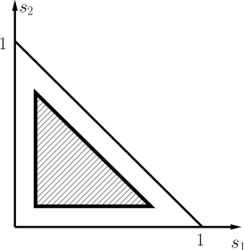
Figure 2: The relevant phase-space region for $(s_{1},s_{2})$ used in this paper is shown by the shaded area.

To exhibit the singularity structure of the virtual corrections discussed in the next section in a transparent way, it is useful to give the leading-order spectrum in $d=4-2\epsilon$ dimensions. We obtain

$$\frac{d\Gamma_{77}^{(0,d)}}{ds_{1}\,ds_{2}}=\frac{\alpha^{2}\,\bar{m}_{b}^{2}(\mu)\,m_{b}^{3}\,|C_{7,eff}(\mu)|^{2}\,G_{F}^{2}\,|V_{tb}V_{ts}^{*}|^{2}\,Q_{d}^{2}}{1024\,\pi^{5}}\,\left(\frac{\mu}{m_{b}}\right)^{4\epsilon}r$$ (2.3)

with

$$r=\frac{\left[r_{0}+\epsilon(r_{1}+r_{2}+r_{3}+r_{4})\right]\left(1-s_{1}-s_{2}\right)}{\left(1-s_{1}\right)^{2}s_{1}\left(1-s_{2}\right)^{2}s_{2}}\,.$$ (2.4)

In $r$ we retained terms of order $\epsilon^{1}$, while discarding terms of higher order. The individual pieces $r_{0},\ldots,r_{4}$ read

$$r_{0} = -48s_{2}^{3}s_{1}^{3}+96s_{2}^{2}s_{1}^{3}-56s_{2}s_{1}^{3}+8s_{1}^{3}+96s_{2}^{3}s_{1}^{2}-192s_{2}^{2}s_{1}^{2}+112s_{2}s_{1}^{2}-56s_{2}^{3}s_{1}+$$ (2.5)

$$112s_{2}^{2}s_{1}-96s_{2}s_{1}+8s_{1}+8s_{2}^{3}+8s_{2}$$

$$r_{1} = -16s_{2}^{2}s_{1}^{3}+16s_{2}s_{1}^{3}-16s_{2}^{3}s_{1}^{2}+48s_{2}^{2}s_{1}^{2}-32s_{2}s_{1}^{2}+16s_{1}^{2}+16s_{2}^{3}s_{1}-$$ (2.6)

$$32s_{2}^{2}s_{1}-16s_{2}s_{1}+16s_{2}^{2}$$

$$r_{2}=-r_{0}\,\log\left(s_{1}\right)\quad;\quad r_{3}=-r_{0}\,\log\left(s_{2}\right)\quad;\quad r_{4}=-r_{0}\,\log\left(1-s_{1}-s_{2}\right)\,.$$ (2.7)

In eq. (2.3) the symbols $\bar{m}_{b}(\mu)$ and $m_{b}$ denote the mass of the $b$-quark in the $\overline{\rm{MS}}$-scheme and in the on-shell scheme, respectively and $C_{7,eff}(\mu)$ is the effective Wilson coefficient of the operator ${\cal O}_{7}$ at the low scale $(\mu\sim m_{b})$, which has an expansion in $\alpha_{s}$ as follows:

$$C_{7,eff}(\mu)=C_{7,eff}^{0}(\mu)+\frac{\alpha_{s}(\mu)}{4\pi}\,C_{7,eff}^{1}(\mu)\,.$$ (2.8)

This Wilson coefficient is known for a long time (see ref. [9] and references therein). Note that in this section only the lowest order part $C_{7,eff}^{0}$ of $C_{7,eff}$ is needed in eq. (2.3), while in the following sections the $C_{7,eff}^{1}$ piece has to be retained.

In $d=4$ dimensions, the leading-order spectrum (in our restricted phase-space) is obtained by simply putting $\epsilon$ to zero, obtaining

$$\frac{d\Gamma_{77}^{(0)}}{ds_{1}\,ds_{2}}=\frac{\alpha^{2}\,\bar{m}_{b}^{2}(\mu)\,m_{b}^{3}\,|C_{7,eff}(\mu)|^{2}\,G_{F}^{2}\,|V_{tb}V_{ts}^{*}|^{2}\,Q_{d}^{2}}{1024\,\pi^{5}}\,\frac{(1-s_{1}-s_{2})}{(1-s_{1})^{2}s_{1}(1-s_{2})^{2}s_{2}}\,r_{0}\,.$$ (2.9)

For completeness, we also list the order $\alpha_{s}^{0}$ result which takes into account the remaining contributions of the operators ${\cal O}_{1}$, ${\cal O}_{2}$ and ${\cal O}_{7}$. Using $\hat{m}_{c}=m_{c}/m_{b}$, one gets [35, 7] when adapted to the operator basis in eq. (1.2)

$$\frac{d\Gamma^{(0)}_{\rm{remaining}}}{ds_{1}ds_{2}}=\frac{\alpha^{2}\,\,m_{b}^{5}\,\,G_{F}^{2}\,|V_{tb}V_{ts}^{*}|^{2}}{1024\,\pi^{5}}\times$$

$$\left\{4\,Q_{u}^{4}\left(C_{2}(\mu)+\frac{4}{3}C_{1}(\mu)\right)^{2}\frac{(s_{1}+s_{2})}{(1-s_{1}-s_{2})^{2}}\left|1-s_{1}-s_{2}-4\,\hat{m}_{c}^{2}\,\arcsin^{2}(z)\right|^{2}\right.$$

$$\left.+16\,Q_{d}\,Q_{u}^{2}\left(C_{2}(\mu)+\frac{4}{3}C_{1}(\mu)\right)\,C_{7,eff}(\mu)\,\left(1-s_{1}-s_{2}-4\,\hat{m}_{c}^{2}\,\mbox{Re}\left(\arcsin^{2}(z)\right)\right)\right\}\,,$$ (2.10)

where we identified $\bar{m}_{b}(\mu)$ with $m_{b}$ (which is correct at lowest order). The argument of the $\arcsin$ function reads $z=\sqrt{(1-s_{1}-s_{2})/(4\,\hat{m}_{c}^{2})}$, where $\hat{m}_{c}^{2}$ is tacitly understood to have a small negative imaginary part.

In Fig. 3 we show the LL results based on eq. (2.9) (dashed line) and the corresponding ones when also including the contributions in eq. (2.10) (solid line). The numerical values of the input parameters and of the Wilson coefficients are listed in tables 1 and 2, respectively. We see that for $\mu=m_{b}/2$ the $({\cal O}_{7},{\cal O}_{7})$ contribution is by far the dominant one. This can be easily understood from eq. (2.10), because the combination $\left(C_{2}(\mu)+\frac{4}{3}C_{1}(\mu)\right)$ is almost zero at this scale. This is no longer true at $\mu=m_{b}$ or $\mu=2m_{b}$, therefore the effects of the remaining terms become more important.

Figure 3: Double differential decay width $d\Gamma^{(0)}/(ds_{1}ds_{2})$ at leading order ($\alpha_{s}^{0}$) as a function of $s_{1}$ for $s_{2}$ fixed at $s_{2}=0.2$. The dashed line shows the result when only the $({\cal O}_{7},{\cal O}_{7})$ interference is taken into account, while the solid line shows all contributions associated with ${\cal O}_{1}$, ${\cal O}_{2}$ and ${\cal O}_{7}$. In the frames 1), 2) and 3) the renormalization scale is chosen to be $\mu=m_{b}/2$, $\mu=m_{b}$ and $\mu=2\,m_{b}$, respectively.

Parameter	Value
$m_{b}$	$4.8$ GeV
$m_{c}/m_{b}$	$0.29$
$m_{t}$	$175$ GeV
$m_{W}$	$80.4$ GeV
$m_{Z}$	$91.19$ GeV
$G_{F}$	$1.16637\times 10^{-5}$ GeV-2
$V_{tb}V_{ts}^{*}$	$0.04$
$V_{cb}$	$0.04$
$\mbox{BR}_{sl}$	$0.1049$
${\alpha}^{-1}$	$137$
${\alpha_{s}(M_{Z})}$	$0.119$

Table 1: Values of the relevant input parameters

	$\alpha_{s}(\mu)$	$C_{7,eff}^{0}(\mu)$	$C_{7,eff}^{1}(\mu)$	$C_{1}^{0}(\mu)$	$C_{2}^{0}(\mu)$
$\mu=m_{W}$	$0.1213$	$-0.1957$	$-2.3835$	$0$	$1$
$\mu=2\,m_{b}$	$0.1818$	$-0.2796$	$-0.1788$	$-0.3352$	$1.0116$
$\mu=m_{b}$	$0.2175$	$-0.3142$	$0.4728$	$-0.4976$	$1.0245$
$\mu=m_{b}/2$	$0.2714$	$-0.3556$	$1.0794$	$-0.7117$	$1.0478$

Table 2: $\alpha_{s}(\mu)$ and the Wilson coefficients $C_{7,eff}^{0}(\mu)$, $C_{7,eff}^{1}(\mu)$, $C_{1}^{0}(\mu)$, $C_{2}^{0}(\mu)$ at different values of the renormalization scale $\mu$.

3 Virtual corrections

We now turn to the calculation of the virtual QCD corrections, i.e. to the contributions of order $\alpha_{s}$ with three particles in the final state. The diagrams defining the (unrenormalized) virtual corrections at the amplitude level are shown in Fig. 4. As the diagrams with a self-energy insertion on the external $b$- and $s$-quark legs are taken into account in the renormalization process, these diagrams are not shown in Fig. 4. In order to get the (unrenormalized) virtual corrections $d\Gamma_{77}^{\rm bare}/(ds_{1}ds_{2})$ of order $\alpha_{s}$ to the decay width, we have to work out the interference of the diagrams in Fig. 4 with the leading order diagrams in Fig. 1.

From the technical point of view, the calculation was made possible by the use of the Laporta Algorithm [36] (see also [37, 38]) to identify the needed Master Integrals and by applying the differential equation method to solve them. As we used these techniques also in [8], we refer to section 7 of that paper which contains the technical details and the corresponding references. In appendix B we present, however, a technical issue which is specific for the present work, viz. a useful parametrization of the three-particle phase-space where one particle is massive.

In addition, we have to work out the counterterm contributions to the decay width. They can be split into two parts, according to

$$\frac{d\Gamma_{77}^{\rm ct}}{ds_{1}ds_{2}}=\frac{d\Gamma_{77}^{{\rm ct},(A)}}{ds_{1}ds_{2}}+\frac{d\Gamma_{77}^{{\rm ct},(B)}}{ds_{1}ds_{2}}\,.$$ (3.1)

Figure 4: The diagrams defining the one-loop amplitude for $b\to s\gamma\gamma$ associated with ${\cal O}_{7}$ are shown. Diagrams with self-energy insertions on the external quark-legs are not shown.

Part (A) involves the Lehmann, Symanzik, Zimmermann (LSZ) factors $\sqrt{Z_{2b}^{\rm OS}}$ and $\sqrt{Z_{2s}^{\rm OS}}$ for the $b$- and $s$-quark field, as well as the self-renormalization constant $Z_{77}^{\overline{\text{MS}}}$ of the operator ${\cal O}_{7}$ and $Z_{m_{b}}^{\overline{\text{MS}}}$ renormalizing the factor $\bar{m}_{b}(\mu)$ present in the operator ${\cal O}_{7}$. The explicit results for these $Z$-factors are given to relevant precision in Appendix C. For part (A) we get

$$\frac{d\Gamma_{77}^{{\rm ct},(A)}}{ds_{1}ds_{2}}=\left[\delta Z_{2b}^{\rm OS}+\delta Z_{2s}^{\rm OS}+2\,\delta Z_{m_{b}}^{\overline{\text{MS}}}+2\,\delta Z_{77}^{\overline{\text{MS}}}\right]\,\frac{d\Gamma_{77}^{(0,d)}}{ds_{1}ds_{2}}\,,$$ (3.2)

where $d\Gamma_{77}^{(0,d)}/(ds_{1}ds_{2})$ is the leading order double differential decay width in $d$-dimensions, as given in eq. (2.3).

Figure 5: Counterterm diagrams with a $\delta m_{b}$ insertion, see text.

The counterterms defining part (B) are due to the insertion of $-i\delta m_{b}\bar{b}b$ in the internal $b$-quark line in the leading order diagrams as indicated in Fig. 5, where

$$\delta m_{b}=(Z_{m_{b}}^{\rm OS}-1)\,m_{b}\,.$$

More precisely, Part (B) consists of the interference of the diagrams in Fig. 5 with the leading order diagrams in Fig. 1. When the strange quark is massive, there is in principle also an analogous insertion of $-i\delta m_{s}\bar{s}s$ in internal $s$-quark lines. $\delta m_{s}$ is, however, proportional to $m_{s}$ and since we neglect terms in which $m_{s}$ appears power-like, we skip this contribution.

By adding $d\Gamma_{77}^{\rm bare}/(ds_{1}ds_{2})$ and $d\Gamma_{77}^{{\rm ct}}/(ds_{1}ds_{2})$, we get the result for the renormalized virtual corrections to the spectrum, $d\Gamma_{77}^{(1),virt}/(ds_{1}\,ds_{2})$. It is useful to decompose this result into two pieces,

$$\frac{d\Gamma_{77}^{(1),virt}}{ds_{1}\,ds_{2}}=\frac{d\Gamma_{77}^{(1,a),virt}}{ds_{1}\,ds_{2}}+\frac{d\Gamma_{77}^{(1,b),virt}}{ds_{1}\,ds_{2}}\,.$$ (3.3)

The infrared- and collinear singularities are completely contained in $d\Gamma_{77}^{(1,a),virt}/(ds_{1}\,ds_{2})$. Explicitly, we obtain (using $x_{4}=m_{s}^{2}/m_{b}^{2}$)

$$\frac{d\Gamma_{77}^{(1,a),virt}}{ds_{1}\,ds_{2}}=\frac{\alpha_{s}}{4\pi}\,C_{F}\,\left[\frac{4\log(s_{1}+s_{2})-4-2\log(x_{4})}{\epsilon}+\log^{2}(x_{4})-\log(x_{4})\right]\,\left(\frac{\mu}{m_{b}}\right)^{2\epsilon}\,\frac{d\Gamma_{77}^{(0,d)}}{ds_{1}\,ds_{2}}$$ (3.4)

where $d\Gamma_{77}^{(0,d)}/(ds_{1}\,ds_{2})$ is understood to be taken exactly as given in eqs. (2.3) and (2.4), i.e., by including the terms of order $\epsilon^{1}$ in $r$. From the explicit expression $d\Gamma_{77}^{(1,a),virt}/(ds_{1}\,ds_{2})$ we see that the singularity structure consists of a simple singular factor multiplying the corresponding tree-level decay width in $d$-dimensions. We stress that the singularities (represented by $1/\epsilon$ poles, $\log(x_{4})$ terms and combinations thereof) are entirely due to soft and/or collinear gluon exchange. The infrared and collinear finite piece $d\Gamma_{77}^{(1,b),virt}/(ds_{1}\,ds_{2})$ can be written as

$$\frac{d\Gamma_{77}^{(1,b),virt}}{ds_{1}\,ds_{2}}=\frac{\alpha^{2}\,\bar{m}_{b}^{2}(\mu)\,m_{b}^{3}\,|C_{7,eff}(\mu)|^{2}\,G_{F}^{2}\,|V_{tb}V_{ts}^{*}|^{2}\,Q_{d}^{2}}{1024\,\pi^{5}}\,\frac{\alpha_{s}}{4\pi}\,C_{F}\times$$

$$\hskip 56.9055pt\left(\frac{-4\,r_{0}\,(1-s_{1}-s_{2})}{(1-s_{1})^{2}\,s_{1}\,(1-s_{2})^{2}\,s_{2}}\,\log\frac{\mu}{m_{b}}+\frac{\sum_{i=1}^{15}\hat{v}_{i}}{3\,(1-s_{1})^{3}\,s_{1}\,(1-s_{2})^{3}\,s_{2}}\right)$$ (3.5)

where the individual quantities $\hat{v}_{1},\ldots,\hat{v}_{15}$ are relegated to Appendix A.

4 Bremsstrahlung corrections

We now turn to the calculation of the bremsstrahlung QCD corrections, i.e. to the contributions of order $\alpha_{s}$ with four particles in the final state. Before going into details, we mention that the kinematical range of the variables $s_{1}$ and $s_{2}$ defined in eq. (2.1) is given in this case by $0\leq s_{1}\leq 1\,;\,0\leq s_{2}\leq 1$. Nevertheless, we consider in this paper only the range which is also accessible to the three-body decay $b\to s\gamma\gamma$, i.e., $0\leq s_{1}\leq 1\,;\,0\leq s_{2}\leq 1-s_{1}$ or, more precisely, by its restricted version specified in eq. (2.2).

The diagrams defining the bremsstrahlung corrections at the amplitude level are shown in Fig. 6.

Figure 6: The diagrams defining the gluon-bremsstrahlung corrections to $b\to s\gamma\gamma$ are shown at the amplitude level. The crosses in the graphs stand for the possible emission places of the gluon.

The amplitude squared, needed to get the (double differential) decay width, can be written as a sum of interferences of the different diagrams in Fig. 6. The four particle final state is described by five independent kinematical variables (see section B.2).

As already mentioned in section 3, the only source of the singularities in the virtual corrections in our restricted range of $s_{1}$ and $s_{2}$ is due to soft gluon-emission and/or collinear emission of gluons from the $s$-quark. When analyzing the bremsstrahlung kinematics, one finds that there are situations where one of the photons can become collinear with the $s$-quark even within the mentioned restricted kinematical range of $s_{1}$ and $s_{2}$. While the singularities related to gluons cancel when combining virtual- and bremsstrahlung corrections, those stemming from collinear photon emission from the $s$-quark will remain and manifest themselves as a term involving a single logarithm $\log(m_{s})$ in the final result.

In our previous paper [8] we realized that for (formally) zero hadronic mass of the $(s,g)$-system collinear photon emission is kinematically impossible. As a consequence, we looked at the triple differential decay width $d\Gamma_{77}/(ds_{1}ds_{2}ds_{3})$, where $s_{3}=(p_{s}+p_{g})^{2}/m_{b}^{2}$ is the normalized hadronic mass squared and found that the double differential decay width, based on the triple differential decay width in which only the leading power terms w.r.t. $s_{3}$ are retained, leads to a nonsingular result when combined with the virtual corrections, which we denoted by $d\Gamma_{77}^{\rm leading\,power}/(ds_{1}ds_{2})$ in ref. [8].

In the present paper, working with a nonzero mass of the strange quark, we go beyond leading power, keeping all terms which are independent of $m_{s}$ and those which involve logarithms of $m_{s}$.

In the present paper we worked out in a first step the triple differential spectrum $d\Gamma_{77}^{(1),brems}/(ds_{1}ds_{2}ds_{3})$, for which we got a fully analytic result, which is however rather lengthy. To get the double differential spectrum $d\Gamma_{77}^{(1),brems}/{ds_{1}ds_{2}}$ we integrated over $s_{3}$, which runs in the interval $[m_{s}^{2}/m_{b}^{2},s_{1}\cdot s_{2}]$. In some terms this integration was done numerically. The final results (after combining with the virtual corrections) are given in a form where certain parts have been fitted to a set of $42$ “basis function”, as the reader will see in the following section.

As the details of the calculations are similar to those in [8], we refer to section 7 of that paper, where the used techniques are described in some detail. In Appendix B we give, however, a useful formula for the parametrization of the $4$-particle phase-space for the case where one of the particles is massive.

5 Final result for the decay width at order $\alpha_{s}$

The complete order $\alpha_{s}$ correction to the double differential decay width $d\Gamma_{77}/(ds_{1}\,ds_{2})$ is obtained by adding the renormalized virtual corrections from section 3 and the bremsstrahlung corrections discussed in section 4. We obtain (using $x_{4}=m_{s}^{2}/m_{b}^{2}$)

$$\frac{d\Gamma_{77}^{(1)}}{ds_{1}\,ds_{2}}=\frac{\alpha^{2}\,\bar{m}_{b}^{2}(\mu)\,m_{b}^{3}\,|C_{7,eff}(\mu)|^{2}\,G_{F}^{2}\,|V_{tb}V_{ts}^{*}|^{2}\,Q_{d}^{2}}{1024\,\pi^{5}}\times$$

$$\hskip 56.9055pt\frac{\alpha_{s}}{4\pi}\,C_{F}\,\,\left[\frac{-4\,r_{0}\,(1-s_{1}-s_{2})}{(1-s_{1})^{2}\,s_{1}\,(1-s_{2})^{2}\,s_{2}}\,\log\frac{\mu}{m_{b}}+f+g\,\log(x_{4})+h\right]\,,$$ (5.1)

where $r_{0}$ is given in eq. (2.5). The first two terms in the square bracket correspond to the leading power result, calculated in the scheme where $m_{s}$ is different from zero, according to the present paper. These two terms are exactly the same as in our previous paper [8] where the leading power terms where calculated in the scheme with $m_{s}=0$. This coincidence, which has to hold of course, provides a nontrivial check of our calculation. The remaining two terms $g$ and $h$ encode all the non-leading power terms which are calculated for the first time in the present paper.

We now turn to the individual terms $f$, $g$ and $h$. As just explained, $f$ is the same as in ref. [8] (see eq. (5.2) there). For $g$ we obtain

$$g= \frac{16\,g_{1}\,\log(s_{1})}{s_{1}(1+s_{1})^{3}(1-s_{2})}+\frac{16\,g_{2}\,\log(s_{2})}{s_{2}(1+s_{2})^{3}(1-s_{1})}+\frac{16\,g_{3}\,\log(1-s_{1})}{s_{2}(1+s_{2})^{3}}+\frac{16\,g_{4}\,\log(1-s_{2})}{s_{1}(1+s_{1})^{3}}+$$ (5.2)

$$\frac{16\,g_{5}\,(s_{1}+s_{2})\,\log(s_{1}+s_{2})+16\,g_{6}\,(1+s_{1})\,(1+s_{2})}{(1-s_{1})s_{1}(1+s_{1})^{3}(1-s_{2})s_{2}(1+s_{2})^{3}(s_{1}+s_{2})}$$

where the functions $g_{1}$,…,$g_{6}$ read

$$g_{1}= -2{s_{1}}^{5}-2{s_{2}}{s_{1}}^{4}-{s_{2}}^{2}{s_{1}}^{3}+2{s_{2}}{s_{1}}^{3}+9{s_{1}}^{3}+{s_{2}}^{2}{s_{1}}^{2}+4{s_{2}}{s_{1}}^{2}+$$ (5.3)

$$17{s_{1}}^{2}+8{s_{2}}{s_{1}}+8{s_{1}}+2{s_{2}}^{2}+2$$

$$g_{2}= g_{1}(s_{1}\leftrightarrow s_{2})$$ (5.4)

$$g_{3}= -2{s_{1}}{s_{2}}^{4}+6{s_{2}}^{4}-4{s_{1}}{s_{2}}^{3}+12{s_{2}}^{3}-4{s_{1}}{s_{2}}^{2}+10{s_{2}}^{2}+{s_{1}}{s_{2}}-{s_{2}}-{s_{1}}-1$$ (5.5)

$$g_{4}= g_{3}(s_{1}\leftrightarrow s_{2})$$ (5.6)

$$g_{5}= -3{s_{2}}^{4}{s_{1}}^{6}-4{s_{2}}^{3}{s_{1}}^{6}-7{s_{2}}^{2}{s_{1}}^{6}-2{s_{1}}^{6}-4{s_{2}}^{5}{s_{1}}^{5}-3{s_{2}}^{4}{s_{1}}^{5}+8{s_{2}}^{3}{s_{1}}^{5}+$$ (5.7)

$$5{s_{2}}^{2}{s_{1}}^{5}-6{s_{1}}^{5}-3{s_{2}}^{6}{s_{1}}^{4}-3{s_{2}}^{5}{s_{1}}^{4}+36{s_{2}}^{4}{s_{1}}^{4}+58{s_{2}}^{3}{s_{1}}^{4}+31{s_{2}}^{2}{s_{1}}^{4}-$$

$$15{s_{2}}{s_{1}}^{4}-8{s_{1}}^{4}-4{s_{2}}^{6}{s_{1}}^{3}+8{s_{2}}^{5}{s_{1}}^{3}+58{s_{2}}^{4}{s_{1}}^{3}+64{s_{2}}^{3}{s_{1}}^{3}+10{s_{2}}^{2}{s_{1}}^{3}-$$

$$32{s_{2}}{s_{1}}^{3}-8{s_{1}}^{3}-7{s_{2}}^{6}{s_{1}}^{2}+5{s_{2}}^{5}{s_{1}}^{2}+31{s_{2}}^{4}{s_{1}}^{2}+10{s_{2}}^{3}{s_{1}}^{2}-46{s_{2}}^{2}{s_{1}}^{2}-$$

$$35{s_{2}}{s_{1}}^{2}-6{s_{1}}^{2}-15{s_{2}}^{4}{s_{1}}-32{s_{2}}^{3}{s_{1}}-35{s_{2}}^{2}{s_{1}}-12{s_{2}}{s_{1}}-2{s_{1}}-$$

$$2{s_{2}}^{6}-6{s_{2}}^{5}-8{s_{2}}^{4}-8{s_{2}}^{3}-6{s_{2}}^{2}-2{s_{2}}$$

$$g_{6}= 4{s_{2}}^{4}{s_{1}}^{6}+{s_{2}}^{3}{s_{1}}^{6}-4{s_{2}}^{2}{s_{1}}^{6}-5{s_{2}}{s_{1}}^{6}+4{s_{1}}^{6}+8{s_{2}}^{5}{s_{1}}^{5}+9{s_{2}}^{4}{s_{1}}^{5}-$$ (5.8)

$$10{s_{2}}^{3}{s_{1}}^{5}-18{s_{2}}^{2}{s_{1}}^{5}+2{s_{2}}{s_{1}}^{5}+9{s_{1}}^{5}+4{s_{2}}^{6}{s_{1}}^{4}+9{s_{2}}^{5}{s_{1}}^{4}-12{s_{2}}^{4}{s_{1}}^{4}-$$

$$29{s_{2}}^{3}{s_{1}}^{4}-14{s_{2}}^{2}{s_{1}}^{4}+22{s_{2}}{s_{1}}^{4}+8{s_{1}}^{4}+{s_{2}}^{6}{s_{1}}^{3}-10{s_{2}}^{5}{s_{1}}^{3}-29{s_{2}}^{4}{s_{1}}^{3}-$$

$$28{s_{2}}^{3}{s_{1}}^{3}+3{s_{2}}^{2}{s_{1}}^{3}+18{s_{2}}{s_{1}}^{3}+5{s_{1}}^{3}-4{s_{2}}^{6}{s_{1}}^{2}-18{s_{2}}^{5}{s_{1}}^{2}-14{s_{2}}^{4}{s_{1}}^{2}+$$

$$3{s_{2}}^{3}{s_{1}}^{2}+12{s_{2}}^{2}{s_{1}}^{2}+3{s_{2}}{s_{1}}^{2}+2{s_{1}}^{2}-5{s_{2}}^{6}{s_{1}}+2{s_{2}}^{5}{s_{1}}+22{s_{2}}^{4}{s_{1}}+$$

$$18{s_{2}}^{3}{s_{1}}+3{s_{2}}^{2}{s_{1}}+4{s_{2}}^{6}+9{s_{2}}^{5}+8{s_{2}}^{4}+5{s_{2}}^{3}+2{s_{2}}^{2}$$

The exact expression for the function $h$ in eq. (5.1) is very lengthy. We therefore write an ansatz of the form

$$h = \frac{\sum_{i=1}^{42}c^{h}_{i}\,u_{i}}{(1-s_{1})^{3}s_{1}(1-s_{2})^{3}s_{2}}\,,$$ (5.9)

where the “basis functions” $u_{i}$ are given in eq. (5) and where the coefficients $c^{h}_{i}$ (see Table 3) are obtained from a fit to the exact function $h$. For simpler use of our results and to make the present paper self-contained, we also provide a fitted version for the function $f$ according to

$$f = \frac{\sum_{i=1}^{42}c^{f}_{i}\,u_{i}}{(1-s_{1})^{3}s_{1}(1-s_{2})^{3}s_{2}}\,.$$ (5.10)

The coefficients $c^{f}_{i}$ are also shown in Table 3. We stress here that the fitted versions of $h$ and $f$ approximate the exact functions very accurately in the whole phase-space, even when choosing the parameter $c$ as small as $1/100$ (see eq. (2.2)).

The basis functions $u_{i}$ (which, like the exact functions $h$ and $f$, are all symmetric in $s_{1}$ and $s_{2}$) are chosen as

$$u_{1}=1,\quad u_{2}={s}_{1}+{s}_{2},\quad u_{3}={s}_{1}^{2}+{s}_{2}^{2},\quad u_{4}={s}_{1}{s}_{2},\quad u_{5}={s}_{1}^{3}+{s}_{2}^{3},\quad u_{6}={s}_{1}^{2}{s}_{2}+{s}_{1}{s}_{2}^{2},$$

$$u_{7}=\log({s}_{1})+\log({s}_{2}),\quad u_{8}={s}_{1}\log({s}_{1})+{s}_{2}\log({s}_{2}),\quad u_{9}={s}_{2}\log({s}_{1})+{s}_{1}\log({s}_{2}),$$

$$u_{10}={s}_{1}^{2}\log({s}_{1})+{s}_{2}^{2}\log({s}_{2}),\quad u_{11}={s}_{1}^{2}\log({s}_{2})+{s}_{2}^{2}\log({s}_{1}),$$

$$u_{12}={s}_{1}{s}_{2}\log({s}_{1})+{s}_{1}{s}_{2}\log({s}_{2}),\quad u_{13}={s}_{1}^{2}{s}_{2}\log({s}_{1})+{s}_{1}{s}_{2}^{2}\log({s}_{2}),$$

$$u_{14}={s}_{1}^{2}{s}_{2}\log({s}_{2})+{s}_{1}{s}_{2}^{2}\log({s}_{1}),\quad u_{15}={s}_{1}^{3}\log({s}_{1})+{s}_{2}^{3}\log({s}_{2}),$$

$$u_{16}={s}_{1}^{3}\log({s}_{2})+{s}_{2}^{3}\log({s}_{1}),\quad u_{17}=\log^{2}({s}_{1})+\log^{2}({s}_{2}),$$

$$u_{18}={s}_{1}\log^{2}({s}_{1})+{s}_{2}\log^{2}({s}_{2}),\quad u_{19}={s}_{2}\log^{2}({s}_{1})+{s}_{1}\log^{2}({s}_{2}),$$

$$u_{20}={s}_{1}^{2}\log^{2}({s}_{1})+{s}_{2}^{2}\log^{2}({s}_{2}),\quad u_{21}={s}_{1}^{2}\log^{2}({s}_{2})+{s}_{2}^{2}\log^{2}({s}_{1}),$$

$$u_{22}={s}_{1}{s}_{2}\log^{2}({s}_{1})+{s}_{1}{s}_{2}\log^{2}({s}_{2}),\quad u_{23}={s}_{1}^{2}{s}_{2}\log^{2}({s}_{1})+{s}_{1}{s}_{2}^{2}\log^{2}({s}_{2}),$$

$$u_{24}={s}_{1}^{2}{s}_{2}\log^{2}({s}_{2})+{s}_{1}{s}_{2}^{2}\log^{2}({s}_{1}),\quad u_{25}={s}_{1}^{3}\log^{2}({s}_{1})+{s}_{2}^{3}\log^{2}({s}_{2}),$$ (5.11)

$$u_{26}={s}_{1}^{3}\log^{2}({s}_{2})+{s}_{2}^{3}\log^{2}({s}_{1}),\quad u_{27}=\log({s}_{1})\log({s}_{2}),$$

$$u_{28}=({s}_{1}+{s}_{2})\log({s}_{1})\log({s}_{2}),\quad u_{29}=\left({s}_{1}^{2}+{s}_{2}^{2}\right)\log({s}_{1})\log({s}_{2}),$$

$$u_{30}={s}_{1}{s}_{2}\log({s}_{1})\log({s}_{2}),\quad u_{31}=\left({s}_{1}^{2}{s}_{2}+{s}_{1}{s}_{2}^{2}\right)\log({s}_{1})\log({s}_{2}),$$

$$u_{32}=\left({s}_{1}^{3}+{s}_{2}^{3}\right)\log({s}_{1})\log({s}_{2}),\quad u_{33}=\log(1-{s}_{1})+\log(1-{s}_{2}),$$

$$u_{34}={s}_{1}\log(1-{s}_{1})+{s}_{2}\log(1-{s}_{2}),\quad u_{35}={s}_{2}\log(1-{s}_{1})+{s}_{1}\log(1-{s}_{2}),$$

$$u_{36}={s}_{1}^{2}\log(1-{s}_{1})+{s}_{2}^{2}\log(1-{s}_{2}),\quad u_{37}={s}_{1}^{2}\log(1-{s}_{2})+{s}_{2}^{2}\log(1-{s}_{1}),$$

$$u_{38}={s}_{1}{s}_{2}\log(1-{s}_{1})+{s}_{1}{s}_{2}\log(1-{s}_{2}),\quad u_{39}={s}_{1}^{2}{s}_{2}\log(1-{s}_{1})+{s}_{1}{s}_{2}^{2}\log(1-{s}_{2}),$$

$$u_{40}={s}_{1}^{2}{s}_{2}\log(1-{s}_{2})+{s}_{1}{s}_{2}^{2}\log(1-{s}_{1}),\quad u_{41}={s}_{1}^{3}\log(1-{s}_{1})+{s}_{2}^{3}\log(1-{s}_{2}),$$

$$u_{42}={s}_{1}^{3}\log(1-{s}_{2})+{s}_{2}^{3}\log(1-{s}_{1}).$$

$i$	$c^{f}_{i}$	$c^{h}_{i}$	$i$	$c^{f}_{i}$	$c^{h}_{i}$
$1$	$1587.9373$	$2808.0884$	$22$	$3839.3787$	$8582.3121$
$2$	$-17820.810$	$-27.836761$	$23$	$2149.8019$	$-3182.8383$
$3$	$5739.2134$	$-127198.90$	$24$	$-2969.4126$	$-3814.5375$
$4$	$79681.671$	$150427.73$	$25$	$1116.5578$	$7876.6985$
$5$	$10672.929$	$123605.68$	$26$	$-51.926335$	$21.979815$
$6$	$-25630.099$	$-61571.822$	$27$	$-6.3461975$	$0.42501969$
$7$	$206.57293$	$370.16329$	$28$	$-198.78562$	$243.20576$
$8$	$-6055.4090$	$-4884.2816$	$29$	$-14.663373$	$3294.2178$
$9$	$-1482.1360$	$261.69714$	$30$	$-5234.3840$	$-11486.898$
$10$	$-13734.475$	$-59064.539$	$31$	$-8078.6742$	$-6953.1246$
$11$	$2458.1907$	$2819.9778$	$32$	$463.51078$	$1842.0350$
$12$	$2578.7004$	$19493.274$	$33$	$-318.01486$	$5524.1650$
$13$	$10698.372$	$29647.891$	$34$	$1007.5887$	$-13495.877$
$14$	$1305.9739$	$4481.7110$	$35$	$17220.702$	$9331.2971$
$15$	$-4990.6306$	$-52868.520$	$36$	$-1072.8013$	$10698.386$
$16$	$-1135.5247$	$-3655.2789$	$37$	$21912.257$	$20102.580$
$17$	$17.550558$	$25.751857$	$38$	$-29656.816$	$-17993.661$
$18$	$-1255.7842$	$-2016.3069$	$39$	$12526.044$	$8586.7318$
$19$	$-97.667743$	$-87.275478$	$40$	$-20491.027$	$-18933.831$
$20$	$-755.27587$	$-18097.634$	$41$	$382.47503$	$-2723.1301$
$21$	$135.25687$	$26.410005$	$42$	$2606.0012$	$2408.5233$

Table 3: Coefficients $c^{f}_{i}$ and $c^{h}_{i}$, which occur in the fits of the functions $f$ and $h$, see eqs. (5.10) and (5.9).

The order $\alpha_{s}$ correction $d\Gamma_{77}^{(1)}/(ds_{1}ds_{2})$ in Eq. (5.1) to the double differential decay width for $b\to X_{s}\gamma\gamma$ is the main result of our paper.

6 Numerical illustrations

In the previous sections we calculated the virtual- and bremsstrahlung QCD corrections associated with the operator ${\cal O}_{7}$. While in the previous paper [8] only the leading power terms in $s_{3}$ ($s_{3}$ is the normalized hadronic mass squared) were taken into account in the underlying triple differential decay width $d\Gamma_{77}/(ds_{1}ds_{2}ds_{3})$, we performed a complete calculation in the present paper. As there are configurations where one of the photons can become collinear with the strange quark, we introduced a finite mass $m_{s}$ which we consider to be of constituent type. While the result based on leading power terms is finite in the limit $m_{s}\to 0$, the full result depends on $m_{s}$ through a single logarithm of the form $\log(x_{4})=\log(m_{s}^{2}/m_{b}^{2})$. In the numerics we will vary $m_{s}$ between $400$ MeV and $600$ MeV.

The NLL prediction reads

$$\frac{d\Gamma_{77}}{ds_{1}ds_{2}}=\frac{d\Gamma_{77}^{(0)}}{ds_{1}ds_{2}}+\frac{d\Gamma_{77}^{(1)}}{ds_{1}ds_{2}}$$ (6.1)

where the first- and second term of the r.h.s. are given in eqs. (2.9) and (5.1), respectively.

To illustrate our results, we first rewrite the $\overline{\mbox{MS}}$ mass $\bar{m}_{b}(\mu)$ in eq. (6.1) in terms of the pole mass $m_{b}$, using the one-loop relation

$$\bar{m}_{b}(\mu)=m_{b}\,\left[1-\frac{\alpha_{s}(\mu)}{4\pi}\,\left(8\log\frac{\mu}{m_{b}}+\frac{16}{3}\right)\right]\,.$$

We then insert $C_{7,eff}(\mu)$ in the expanded form (2.8) and expand the resulting expression for $d\Gamma_{77}/(ds_{1}ds_{2})$ w.r.t. $\alpha_{s}$, discarding terms of order $\alpha_{s}^{2}$. This procedure defines the full NLL result and also the version where only the leading power terms are retained in $d\Gamma^{(1)}_{77}/(ds_{1}ds_{2})$. The corresponding LL result is obtained by discarding the order $\alpha_{s}^{1}$ term. The numerical values for the input parameters and for this Wilson coefficient at various values for the scale $\mu$, together with the numerical values of $\alpha_{s}(\mu)$, are given in Table 1 and Table 2, respectively.

In Fig. 7 the LL result, the NLL result based on the leading power contribution and the full NLL result are shown by the dotted, the dashed and the solid lines, respectively. Among the three solid lines, the highest, middle and lowest curve correspond to $m_{s}=400$ MeV, $m_{s}=500$ MeV and $m_{s}=600$ MeV, respectively.

From Fig. 7, where $s_{2}$ is fixed at $s_{2}=0.2$, we see that for $s_{1}\leq 0.4$ the NLL result is dominated by the leading power result obtained in our previous paper [8], while this is no longer true for larger values of $s_{1}$. In these plots $s_{1}=0.8$ corresponds to the maximal value of the leading order kinematics. In other words the point $(s_{1}=0.8,s_{2}=0.2)$ lies on the “diagonal line” characterized by $1-s_{1}-s_{2}=0$ in Fig. 2. That is why the dotted curves becomes zero at $s_{1}=0.8$. This also holds for the virtual corrections which have the same kinematical range. The full kinematical range in the $(s_{1},s_{2})$-plane for the bremsstrahlung process is, however, larger than the window considered in this paper. For this reason the solid lines do not go to zero at $s_{1}=0.8$. However, the leading power terms of the bremsstrahlung corrections have similar features as the virtual corrections and go to zero for $s_{1}=0.8$ (as seen from the dashed curves). A more detailed investigation shows that the leading power contributions only give a good approximation of the NLL result when one is sufficiently away from the line $1-s_{1}-s_{2}=0$ in the $(s_{1},s_{2})$-plane.

The comparison of the full NLL corrections with the corresponding leading power pieces is basically of “historic” interest; it is more important to compare the LL curves (dotted) with the full NLL ones (solid). Form Fig. 7 one concludes that the NLL corrections to the ${\cal O}_{7}$ are crucial. We stress that the QCD corrections involving the operators ${\cal O}_{1}$ and ${\cal O}_{2}$, which we did not consider in our paper, also will be important. Therefore, the issue concerning the reduction of the $\mu$ dependence at NLL precision cannot be addressed in a meaningful way at this level.

To get the branching ratio for $\bar{B}\to X_{s}\gamma\gamma$ as a function of the cut-off parameter $c$ defined in eq. (2.2), we integrate the double differential spectrum over the corresponding range in $s_{1}$ and $s_{2}$, divide by the semileptonic decay width and multiply with the measured semileptonic branching ratio. For the purpose of this paper it is sufficient to take the lowest order formula for the semileptonic decay width, reading

$$\Gamma_{sl}=\frac{m_{b}^{5}\,G_{F}^{2}\,|V_{cb}|^{2}}{192\pi^{3}}\,g(m_{c}/m_{b})\,,$$ (6.2)

with the phase space factor

$$g(z)=1-8\,z^{2}+8\,z^{6}-z^{8}-24\,z^{4}\log(z)\,.$$ (6.3)

Figure 7: Double differential decay width $d\Gamma_{77}/(ds_{1}ds_{2})$, based on the operator ${\cal O}_{7}$ only, as a function of $s_{1}$ for $s_{2}$ fixed at $s_{2}=0.2$. The dotted, the dashed and the solid lines show the LL result, the NLL when only retaining leading power terms as in ref. [8] and the full NLL result of the present paper, respectively. Among the three solid lines, the highest, middle and lowest curve correspond to $m_{s}=400$ MeV, $m_{s}=500$ MeV and $m_{s}=600$ MeV, respectively. In the frames 1), 2) and 3) the renormalization scale is chosen to be $\mu=m_{b}/2$, $\mu=m_{b}$ and $\mu=2\,m_{b}$, respectively. See text for details.

Using the input parameters in Tables 1 and 2, we get the branching ratios shown in Table 4 for the values $c=1/100$ (upper half) and $c=1/50$ (lower half) at $\mu=m_{b}/2$, $\mu=m_{b}$ and $\mu=2m_{b}$. In the columns “${\cal O}_{7}$” only the operator ${\cal O}_{7}$ is taken into account, while the number in the columns “all” also takes into account the lowest order contributions involving the operators ${\cal O}_{1}$ and ${\cal O}_{2}$ (according to eq. (2.10)).

	${\cal O}_{7}$	all	${\cal O}_{7}$	all	${\cal O}_{7}$	all
	$\mu=m_{b}/2$	$\mu=m_{b}/2$	$\mu=m_{b}$	$\mu=m_{b}$	$\mu=2m_{b}$	$\mu=2m_{b}$
LL	3.96	3.96	3.10	3.11	2.45	2.53
$\mbox{NLL}_{1}$	3.81	3.81	2.37	2.39	1.60	1.68
$\mbox{NLL}_{2}$	3.35	3.34	2.08	2.10	1.41	1.49
$\mbox{NLL}_{3}$	2.97	2.97	1.85	1.87	1.25	1.33
LL	2.40	2.40	1.87	1.89	1.48	1.55
$\mbox{NLL}_{1}$	2.39	2.39	1.49	1.51	1.01	1.08
$\mbox{NLL}_{2}$	2.17	2.17	1.35	1.37	0.91	0.99
$\mbox{NLL}_{3}$	1.99	1.99	1.24	1.26	0.84	0.91

Table 4: Branching ratios for $\bar{B}\to X_{s}\gamma\gamma$ in units of $10^{-7}$. The upper half of the table is for $c=1/100$ and lower half for $c=1/50$. LL is the leading logarithmic result. $\mbox{NLL}_{1}$, $\mbox{NLL}_{2}$ and $\mbox{NLL}_{3}$ are the results where the NLL corrections to the ${\cal O}_{7}$ contributions are included, using $m_{s}=400$ MeV, $m_{s}=500$ MeV and $m_{s}=600$ MeV, respectively. See text for more information.

7 Summary

In the present work we calculated the $O(\alpha_{s})$ corrections to the decay process $\bar{B}\to X_{s}\gamma\gamma$ originating from diagrams involving the electromagnetic dipole operator ${\cal O}_{7}$. This calculation involves contributions with three particles in the final state and a gluon in the loop (virtual corrections) and tree-level contributions with four particles in the final state (gluon bremsstrahlung corrections).

We introduced a nonzero mass $m_{s}$ for the strange quark to regulate configurations where the gluon or one of the photons become collinear with the strange quark and retained terms which are logarithmic in $m_{s}$, while discarding terms which go to zero in the limit $m_{s}\to 0$. When combining virtual- and bremsstrahlung corrections, the infrared and collinear singularities induced by soft and/or collinear gluons drop out. By our cuts the photons do not become soft, but one of them can become collinear with the strange quark. This implies that in the final result a single logarithms of $m_{s}$ survives. We interpret $m_{s}$ appearing in the result as a constituent mass and vary it between $400$ MeV and $600$ MeV in the numerics.

We find that the NLL corrections to the double differential spectrum $d\Gamma_{77}/(ds_{1}ds_{2})$ are large in general. Depending on the point in the $(s_{1},s_{2})$-plane, they can modify the LL predictions by up to $50\%$ in both directions, which means that not only the normalization, but also the shapes of the distributions are modified, as can be seen e.g. in Figure 7.

We also compared our new results with those obtained in an earlier paper [8], where only the leading power terms w.r.t. $s_{3}$ in the underlying triple differential spectrum $d\Gamma_{77}/(ds_{1}ds_{2}ds_{3})$ were retained.

Appendix A Explicit results for the functions $\hat{v}_{i}$ defining the virtual corrections

The functions $\hat{v}_{i}$ appearing in eq. (3.5) read

$$\hat{v}_{1} = 16(1-s_{1}-s_{2})\left[\left(96-2\pi^{2}\right)s_{1}^{4}s_{2}^{4}+\left(11\pi^{2}-291\right)s_{1}^{4}s_{2}^{3}+\left(300-19\pi^{2}\right)s_{1}^{4}s_{2}^{2}+\right.$$

$$\left.\left(12\pi^{2}-117\right)s_{1}^{4}s_{2}+\left(12-3\pi^{2}\right)s_{1}^{4}+\left(11\pi^{2}-291\right)s_{1}^{3}s_{2}^{4}+\left(894-36\pi^{2}\right)s_{1}^{3}s_{2}^{3}+\right.$$

$$\left.\left(48\pi^{2}-936\right)s_{1}^{3}s_{2}^{2}+\left(348-21\pi^{2}\right)s_{1}^{3}s_{2}+\left(2\pi^{2}-15\right)s_{1}^{3}+\left(300-19\pi^{2}\right)s_{1}^{2}s_{2}^{4}+\right.$$

$$\left.\left(48\pi^{2}-936\right)s_{1}^{2}s_{2}^{3}+\left(1044-60\pi^{2}\right)s_{1}^{2}s_{2}^{2}+\left(26\pi^{2}-426\right)s_{1}^{2}s_{2}+\left(18-\pi^{2}\right)s_{1}^{2}-\right.$$

$$\left.\pi^{2}\left(s_{1}^{5}s_{2}^{3}-3s_{1}^{5}s_{2}^{2}+3s_{1}^{5}s_{2}-s_{1}^{5}+s_{1}^{3}s_{2}^{5}-3s_{1}^{2}s_{2}^{5}+3s_{1}s_{2}^{5}-s_{2}^{5}\right)+\right.$$

$$\left.\left(12\pi^{2}-117\right)s_{1}s_{2}^{4}+\left(348-21\pi^{2}\right)s_{1}s_{2}^{3}+\left(26\pi^{2}-426\right)s_{1}s_{2}^{2}+\left(210-14\pi^{2}\right)s_{1}s_{2}+\right.$$

$$\left.\left(\pi^{2}-15\right)s_{1}+\left(12-3\pi^{2}\right)s_{2}^{4}+\left(2\pi^{2}-15\right)s_{2}^{3}+\left(18-\pi^{2}\right)s_{2}^{2}+\left(\pi^{2}-15\right)s_{2}\right]$$

$$\hat{v}_{2} = -96s_{1}s_{2}\left(1-s_{1}\right)^{3}\left(1-s_{2}\right)^{2}\left(1-s_{1}-s_{2}\right)\left(2-3s_{2}\right)\,\log\left(s_{1}\right)$$

$$\hat{v}_{3} = 48s_{1}s_{2}\left(1-s_{1}\right)^{2}\left(1-s_{2}\right)^{2}\left(1-s_{1}-s_{2}\right)\left(s_{1}-s_{1}^{2}+2s_{2}-s_{1}s_{2}\right)\log^{2}\left(s_{1}\right)$$

$$\hat{v}_{4} = -96\left(1-s_{1}\right){}^{2}\left(1-s_{2}\right){}^{2}s_{2}\left(s_{1}^{4}+2s_{2}s_{1}^{3}-2s_{1}^{3}+s_{2}^{2}s_{1}^{2}-4s_{2}s_{1}^{2}+s_{1}^{2}-2s_{2}^{2}s_{1}+\right.$$

$$\left.3s_{2}s_{1}-2s_{1}+s_{2}^{2}+1\right)\log\left(s_{1}\right)\log\left(s_{1}+s_{2}\right)$$

$$\hat{v}_{5} = 48\left(1-s_{1}\right)\left(s_{2}-1\right){}^{2}s_{2}\left(1-s_{1}-s_{2}\right)\left(6s_{2}s_{1}^{3}-6s_{1}^{3}-11s_{2}s_{1}^{2}+15s_{1}^{2}+\right.$$

$$\left.3s_{2}s_{1}-9s_{1}+2\right)\log\left(1-s_{1}\right)$$

$$\hat{v}_{6} = 96\left(1-s_{1}\right)\left(s_{2}-1\right){}^{2}\left(s_{2}s_{1}^{5}-s_{1}^{5}+2s_{2}^{2}s_{1}^{4}-5s_{2}s_{1}^{4}+3s_{1}^{4}+s_{2}^{3}s_{1}^{3}-5s_{2}^{2}s_{1}^{3}+\right.$$

$$\left.8s_{2}s_{1}^{3}-2s_{1}^{3}-s_{2}^{3}s_{1}^{2}+4s_{2}^{2}s_{1}^{2}-4s_{2}s_{1}^{2}+s_{1}^{2}-4s_{2}^{2}s_{1}+3s_{2}s_{1}-s_{1}-s_{2}^{2}+s_{2}\right)\times$$

$$\log\left(1-s_{1}\right)\log\left(s_{1}+s_{2}\right)$$

$$\hat{v}_{7} = 48\left(1-s_{1}\right)\left(1-s_{2}\right)\left(s_{2}^{2}s_{1}^{5}-s_{2}s_{1}^{5}-9s_{2}^{3}s_{1}^{4}+16s_{2}^{2}s_{1}^{4}-8s_{2}s_{1}^{4}+s_{1}^{4}-9s_{2}^{4}s_{1}^{3}+\right.$$

$$\left.46s_{2}^{3}s_{1}^{3}-67s_{2}^{2}s_{1}^{3}+35s_{2}s_{1}^{3}-s_{1}^{3}+s_{2}^{5}s_{1}^{2}+16s_{2}^{4}s_{1}^{2}-67s_{2}^{3}s_{1}^{2}+84s_{2}^{2}s_{1}^{2}-\right.$$

$$\left.43s_{2}s_{1}^{2}+s_{1}^{2}-s_{2}^{5}s_{1}-8s_{2}^{4}s_{1}+35s_{2}^{3}s_{1}-43s_{2}^{2}s_{1}+22s_{2}s_{1}-s_{1}+s_{2}^{4}-s_{2}^{3}+\right.$$

$$\left.s_{2}^{2}-s_{2}\right)\log^{2}\left(s_{1}+s_{2}\right)$$

$$\hat{v}_{8} = 96s_{1}\left(1-s_{2}\right){}^{2}\left(1-s_{1}-s_{2}\right)\left(s_{2}s_{1}^{4}-s_{1}^{4}+s_{2}^{2}s_{1}^{3}-4s_{2}s_{1}^{3}+3s_{1}^{3}-5s_{2}^{2}s_{1}^{2}+\right.$$

$$\left.8s_{2}s_{1}^{2}-2s_{1}^{2}+7s_{2}^{2}s_{1}-11s_{2}s_{1}+s_{1}-2s_{2}^{2}+5s_{2}-1\right)\text{Li}_{2}\left(s_{1}\right)$$

$$\hat{v}_{9} = 96\left(1-s_{1}\right)\left(1-s_{2}\right)\left(1-s_{1}-s_{2}\right)\left(s_{2}^{2}s_{1}^{4}-2s_{2}s_{1}^{4}+s_{1}^{4}+8s_{2}^{3}s_{1}^{3}-17s_{2}^{2}s_{1}^{3}+\right.$$

$$\left.12s_{2}s_{1}^{3}-3s_{1}^{3}+s_{2}^{4}s_{1}^{2}-17s_{2}^{3}s_{1}^{2}+32s_{2}^{2}s_{1}^{2}-20s_{2}s_{1}^{2}-2s_{2}^{4}s_{1}+12s_{2}^{3}s_{1}-\right.$$

$$\left.20s_{2}^{2}s_{1}+20s_{2}s_{1}-2s_{1}+s_{2}^{4}-3s_{2}^{3}-2s_{2}\right)\text{Li}_{2}\left(1-s_{1}-s_{2}\right)$$

$$\hat{v}_{10}=\hat{v}_{2}(s_{1}\leftrightarrow s_{2})\quad\quad\hat{v}_{11}=\hat{v}_{3}(s_{1}\leftrightarrow s_{2})\quad\quad\hat{v}_{12}=\hat{v}_{4}(s_{1}\leftrightarrow s_{2})\quad\quad$$

$$\hat{v}_{13}=\hat{v}_{5}(s_{1}\leftrightarrow s_{2})\quad\quad\hat{v}_{14}=\hat{v}_{6}(s_{1}\leftrightarrow s_{2})\quad\quad\hat{v}_{15}=\hat{v}_{8}(s_{1}\leftrightarrow s_{2})$$ (A.1)

Appendix B Relevant phase-space formulas

The fully differential decay width $d\Gamma$ for a generic process $p\to p_{1}+p_{2}+...+p_{n}$ can be written as

$$d\Gamma=\frac{1}{2m}\,\overline{|M|^{2}}\,D\Phi(1\to n)\,,$$ (B.1)

where $\overline{|M|^{2}}$ is the squared matrix element, summed and averaged over spins and colors of the particles in the final and initial state, respectively, and $m$ is the mass of the decaying particle.

In ref. [39] useful parametrizations for the phase-space factors $D\Phi(1\to n)$ have been given for $n=3,4$, for the case when all final-state particles are massive. Among the final-state particles only the strange quark is massive in our application, which means that the general formulas simplify. In the following subsections we see that the 3-particle phase-space can be parametrized in terms of two parameters $\lambda_{1}$ and $\lambda_{2}$, which run independently in the range $[0,1]$, while five such parameters ($\lambda_{1},...,\lambda_{5}$) are involved in the 4-particle phase-space. Of course, all scalar products involved in $\overline{|M|^{2}}$ can be expressed in terms of these parameters.

B.1 Phase-space parametrization for the 3-particle final state

In our application we identify $p_{1}$ with the strange quark and $p_{2},p_{3}$ with the two photons and define $x_{1}=m_{s}^{2}/m_{b}^{2}$. Starting from eq. (2.10) of ref. [39], one gets

$$D\Phi(1\to 3)= \frac{{m}_{b}^{2d-6}2^{1-2d}\pi^{1-d}}{\Gamma(d-2)}[(1-\lambda_{1})\lambda_{1}]^{\frac{d-4}{2}}[(1-\lambda_{2})\lambda_{2}]^{d-3}\times$$ (B.2)

$$(1-{x}_{1})^{2d-5}[\lambda_{2}(1-{x}_{1})+{x}_{1}]^{\frac{2-d}{2}}\,d\lambda_{1}d\lambda_{2}\,.$$

The scalar products of the momenta $p_{i}$, encoded in the quantities $s_{ij}=(p_{i}+p_{j})^{2}/m_{b}^{2}$, can be written in terms of the parameters $\lambda_{1}$ and $\lambda_{2}$ as

$$s_{13} = \lambda_{2}(1-{x}_{1})+{x}_{1}$$

$$s_{12} = \frac{\lambda_{1}(\lambda_{2}-1)\lambda_{2}(1-{x}_{1})^{2}-{x}_{1}}{\lambda_{2}({x}_{1}-1)-{x}_{1}}\,.$$

From the observation that $s_{1}=s_{13}$ and $s_{2}=s_{12}$ one easily gets the expression for the double differential spectrum $d\Gamma/(ds_{1}ds_{2})$.

B.2 Phase-space parametrization for the 4-particle final state

In our application we identify $p_{1},p_{2}$ with the two photons, $p_{3}$ with the gluon and $p_{4}$ with the strange quark and define $x_{4}=m_{s}^{2}/m_{b}^{2}$. Starting then from eq. (3.10) of ref. [39], putting there $x_{1}=x_{2}=x_{3}=0$ and performing the substitutions

$$z_{1}=2\lambda_{3}-1,\quad{z}_{32}=2\lambda_{5}-1,\quad{s}_{234}=\lambda_{1}(1-{x}_{4})+{x}_{4}\,$$

$$E_{2}=\frac{\lambda_{1}(1-\lambda_{2})(1-{x}_{4})}{2\sqrt{\lambda_{1}+{x}_{4}-\lambda_{1}{x}_{4}}}\,,$$ (B.3)

$${z}_{31}=\frac{\lambda_{1}(1-{x}_{4})(\lambda_{2}(1-\lambda_{4})-\lambda_{4})+(1-2\lambda_{4}){x}_{4}}{\lambda_{1}(1-{x}_{4})(\lambda_{2}(1-\lambda_{4})+\lambda_{4})+{x}_{4}}\,,$$

we get the following expression for the phase-space factor:

$$D\Phi(1\to 4) = (4\pi)^{-\frac{3d}{2}}m_{b}^{3d-8}\frac{2^{2d-7}\Gamma(\frac{d-2}{2})}{(d-3)\Gamma(d-3)^{2}}(1-{x}_{4})^{3d-7}[(1-\lambda_{1})(1-\lambda_{2})\lambda_{2}]^{d-3}$$

$$\times \lambda_{1}^{2d-5}[(\lambda_{1}(1-{x}_{4})+{x}_{4})(\lambda_{1}\lambda_{2}(1-{x}_{4})+{x}_{4})]^{1-\frac{d}{2}}$$

$$\times [(1-\lambda_{3})\lambda_{3}(1-\lambda_{4})\lambda_{4}]^{\frac{d}{2}-2}[(1-\lambda_{5})\lambda_{5}]^{\frac{d-5}{2}}\,d\lambda_{1}d\lambda_{2}d\lambda_{3}d\lambda_{4}d\lambda_{5}\,.$$

As mentioned above, all $\lambda_{i}$ run independently in the range $[0,1]$. All scalar products of the momenta $p_{i}$, encoded in the quantities $s_{ij}=(p_{i}+p_{j})^{2}/m_{b}^{2}$ and $s_{ijk}=(p_{i}+p_{j}+p_{k})^{2}/m_{b}^{2}$, can be written in terms of the parameters $\lambda_{1},...,\lambda_{5}$ as

$$s_{234} = \lambda_{1}(1-{x}_{4})+{x}_{4}\,,$$

$$s_{34} = \lambda_{1}\lambda_{2}(1-{x}_{4})+{x}_{4}\,,$$

$$s_{23} = \frac{\lambda_{1}^{2}(1-\lambda_{2})\lambda_{2}\lambda_{4}(1-{x}_{4})^{2}}{\lambda_{1}\lambda_{2}(1-{x}_{4})+{x}_{4}}\,,$$ (B.5)

$$s_{134} = \frac{\lambda_{1}(1-{x}_{4})[\lambda_{2}(1-(1-\lambda_{1})\lambda_{3}(1-{x}_{4}))+\lambda_{3}(1-\lambda_{1})(1-{x}_{4})]+{x}_{4}}{\lambda_{1}(1-{x}_{4})+{x}_{4}}\,,$$

$$s_{13} = (s_{13}^{+}-s_{13}^{-})\lambda_{5}+s_{13}^{-}\,,$$

where

$$s_{13}^{\pm} = \frac{(1-\lambda_{1})\lambda_{1}\lambda_{2}(1-{x}_{4})^{2}}{(\lambda_{1}+{x}_{4}-\lambda_{1}{x}_{4})(\lambda_{1}\lambda_{2}+{x}_{4}-\lambda_{1}\lambda_{2}{x}_{4})}\left\{{x}_{4}[(1-\lambda_{3})(1-\lambda_{4})+\lambda_{3}\lambda_{4}]\right.$$

$$+ \left.(1-{x}_{4})\lambda_{1}[\lambda_{2}(1-\lambda_{3})(1-\lambda_{4})+\lambda_{3}\lambda_{4}]\right.$$

$$\mp \left.2\sqrt{(1-\lambda_{3})\lambda_{3}(1-\lambda_{4})\lambda_{4}(\lambda_{1}+{x}_{4}-\lambda_{1}{x}_{4})(\lambda_{1}\lambda_{2}+{x}_{4}-\lambda_{1}\lambda_{2}{x}_{4})}\right\}\,.$$

From the observation that $s_{1}=s_{234}$, $s_{2}=s_{134}$ and $s_{3}=s_{34}$ one easily gets the expression for the triple differential spectrum $d\Gamma/(ds_{1}ds_{2}ds_{3})$.

Appendix C Renormalization constants

In this appendix, we collect the explicit expressions of the renormalization constants needed for the ultraviolet renormalization in our calculation (see section 3).

The operator ${\cal O}_{7}$, as well as the $b$-quark mass contained in this operator are renormalized in the $\overline{\text{MS}}$ scheme [40]:

$$Z_{77}^{\overline{\text{MS}}}=1+\frac{4\,C_{F}}{\epsilon}\frac{\alpha_{s}(\mu)}{4\pi}+O(\alpha_{s}^{2})\quad;\quad Z_{m_{b}}^{\overline{\text{MS}}}=1-\frac{3\,C_{F}}{\epsilon}\frac{\alpha_{s}(\mu)}{4\pi}+O(\alpha_{s}^{2})\,.$$ (C.1)

All the remaining fields and parameters are renormalized in the on-shell scheme. The on-shell renormalization constant for the $b$-quark mass is given by

$$Z_{m_{b}}^{\rm OS}=1-C_{F}\,\Gamma(\epsilon)\,e^{\gamma\epsilon}\,\frac{3-2\epsilon}{1-2\epsilon}\left(\frac{\mu}{m_{b}}\right)^{2\epsilon}\frac{\alpha_{s}(\mu)}{4\pi}+O(\alpha_{s}^{2})\,.$$ (C.2)

while the renormalization constants for the $s$- and $b$-quark fields are ($q=b$ or $q=s$)

$$Z_{2q}^{\rm OS} = 1-C_{F}\,\Gamma(\epsilon)\,e^{\gamma\epsilon}\,\frac{3-2\epsilon}{1-2\epsilon}\left(\frac{\mu}{m_{q}}\right)^{2\epsilon}\frac{\alpha_{s}(\mu)}{4\pi}+O(\alpha_{s}^{2})\,.$$ (C.3)

The various quantities $\delta Z$ appearing in section 3 are defined to be $\delta Z=Z-1$.

References

[1]
M. Misiak et al.,
Phys. Rev. Lett. 98 (2007) 022002,
[hep-ph/0609232].
[2]
T. Hurth, M. Nakao,
Ann. Rev. Nucl. Part. Sci. 60 (2010) 645,
[arXiv:1005.1224 [hep-ph]].
[3]
A. J. Buras,
arXiv:1102.5650 [hep-ph].
[4]
H. Simma, D. Wyler,
Nucl. Phys. B344 (1990) 283.
[5]
L. Reina, G. Ricciardi, A. Soni,
Phys. Lett. B396 (1997) 231,
[hep-ph/9612387].
[6]
L. Reina, G. Ricciardi, A. Soni,
Phys. Rev. D56 (1997) 5805,
[hep-ph/9706253].
[7]
J. J. Cao, Z.J. Xiao, G. R. Lu,
Phys. Rev. D64 (2001) 014012,
[hep-ph/0103154].
[8]
H. M. Asatrian, C. Greub, A. Kokulu and A. Yeghiazaryan,
Phys. Rev. D 85 (2012) 014020
[arXiv:1110.1251 [hep-ph]].
[9]
K. G. Chetyrkin, M. Misiak and M. Munz,
Phys. Lett. B 400 (1997) 206
[Erratum-ibid. B 425 (1998) 414],
[arXiv:hep-ph/9612313].
[10]
K. Melnikov and A. Mitov, Phys. Lett. B 620 (2005) 69,
[arXiv:hep-ph/0505097].
[11]
H. M. Asatrian, T. Ewerth, A. Ferroglia, P. Gambino, C. Greub,
Nucl. Phys. B762 (2007) 212,
[hep-ph/0607316].
[12]
A. Kapustin, Z. Lint and H. D. Politzer,
Phys. Lett. B 357 (1995) 653,
[arXiv:hep-ph/9507248].
[13]
H. M. Asatrian and C. Greub,
Phys. Rev. D 88 (2013) 074014
[arXiv:1305.6464 [hep-ph]].
[14]
M. Kaminski, M. Misiak and M. Poradzinski,
Phys. Rev. D 86 (2012) 094004
[arXiv:1209.0965 [hep-ph]].
[15]
A. Gemintern, S. Bar-Shalom, G. Eilam,
Phys. Rev. D70 (2004) 035008,
[hep-ph/0404152].
[16]
C. -H. V. Chang, G. -L. Lin, Y. -P. Yao,
Phys. Lett. B415 (1997) 395,
[hep-ph/9705345].
[17]
G. Hiller, E. O. Iltan,
Phys. Lett. B409 (1997) 425,
[hep-ph/9704385].
[18]
S. W. Bosch, G. Buchalla,
JHEP 0208 (2002) 054,
[hep-ph/0208202].
[19]
S. W. Bosch,
hep-ph/0208203.
[20]
G. Hiller, A. S. Safir,
JHEP 0502 (2005) 011,
[hep-ph/0411344].
[21]
G. Hiller, A. S. Safir,
PoS HEP2005 (2006) 277,
[hep-ph/0511316].
[22]
G. L. Lin, J. Liu and Y. P. Yao,
Phys. Rev. Lett. 64 (1990) 1498.
[23]
S. Herrlich and J. Kalinowski,
Nucl. Phys. B 381 (1992) 501.
[24]
S. R. Choudhury, G. C. Joshi, N. Mahajan, B. H. J. McKellar,
Phys. Rev. D67 (2003) 074016,
[hep-ph/0210160].
[25]
T. M. Aliev, G. Hiller, E. O. Iltan,
Nucl. Phys. B515 (1998) 321,
[hep-ph/9708382].
[26]
S. Bertolini, J. Matias,
Phys. Rev. D57 (1998) 4197,
[hep-ph/9709330].
[27]
I. I. Bigi, G. Chiladze, G. Devidze, C. Hanhart, A. Liparteliani, U. -G. Meissner,
hep-ph/0603160.
[28]
G. G. Devidze, G. R. Jibuti,
hep-ph/9810345.
[29]
T. M. Aliev, G. Turan,
Phys. Rev. D48 (1993) 1176.
[30]
Z. J. Xiao, C. D. Lu, W. J. Huo,
Phys. Rev. D67 (2003) 094021, [hep-ph/0301221].