Large deviations of spread measures for Gaussian matrices

Abstract

For a large $n\times m$ Gaussian matrix, we compute the joint statistics, including large deviation tails, of generalized and total variance - the scaled log-determinant $H$ and trace $T$ of the corresponding $n\times n$ covariance matrix. Using a Coulomb gas technique, we find that the Laplace transform of their joint distribution $\mathcal{P}_{n}(h,t)$ decays for large $n,m$ (with $c=m/n\geq 1$ fixed) as $\hat{\mathcal{P}}_{n}(s,w)\approx\exp\left(-\beta n^{2}J(s,w)\right)$, where $\beta$ is the Dyson index of the ensemble and $J(s,w)$ is a $\beta$-independent large deviation function, which we compute exactly for any $c$. The corresponding large deviation functions in real space are worked out and checked with extensive numerical simulations. The results are complemented with a finite $n,m$ treatment based on the Laguerre-Selberg integral. The statistics of atypically small log-determinants is shown to be driven by the split-off of the smallest eigenvalue, leading to an abrupt change in the large deviation speed.

1 Introduction

The standard deviation $\sigma$ of an array of $m$ data $X_{i}$ is the simplest measure of how spread these numbers are around their average value $\bar{X}=(1/m)\sum_{i=1}^{m}X_{i}$. Suppose that the $X_{i}$’s represent the final ‘Physics’ marks of $m$ students of a high-school. Most worrisome scenarios for the headmaster would be a low $\bar{X}$ and/or a high $\sigma$, signaling an overall poor and/or highly non-uniform performance.

What if ‘Physics’ and ‘Arts’ marks are collected together? Detecting performance issues now immediately becomes a much harder task, as data may fluctuate together and in different directions. A two-dimensional scatter plot may help, though. The “centre" of the cloud gives a rough indication of how well the students perform on average in both subjects. But how to tell in which subject the gap between excellent and mediocre students is more pronounced, or whether outstanding students in one subject also excel in the other?

In Fig. 1 (Bottom) we sketch two scatter plots of marks adjusted to have zero mean. A meaningful spread indicator seems to be the shape of the ellipse enclosing each cloud. For example, an almost circular cloud - like School $1$ - represents a rather uninformative situation, where your ‘Arts’ marks tell nothing about your ‘Physics’ skills, and vice versa. Conversely, a rather elongated shape - like School $2$ - highlights correlations between each student’s marks in different subjects.

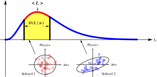
Figure 1: (color online) Top: Sketch of the probability density of the likelihood ratio $L$ of a Gaussian iid data set. In yellow, the typical region around the mean of order $\mathcal{O}(1/n)$. Larger fluctuations are referred to as atypical large deviations. Bottom: Sketch of two multivariate data sets with $n=2$ and $m=35$. Each point represents a student, for two different schools, and his/her marks in Arts and Physics. The two datasets have same generalized variance $H$, but different total variance $T$. The likelihood ratio $L$ of School 1 is compatible with the iid hypothesis, while the value of $L$ for School $2$ is atypically far from the average $\left<L\right>$.

For a bunch of many scattered points it would be desirable to summarize the overall spread around the mean just by a single scalar quantity, like the perimeter or area of the enclosing ellipse. Not surprisingly, however, these indicators (taken individually) have evident shortcomings [30]. Surely a wiser choice is to combine more than a single spread measure (like perimeter or area alone), to obtain a more revealing indicator. These issues arise naturally in multivariate statistics, and more mathematical tools and techniques are required compared to the univariate setting.

In this work, we compute the joint statistics of “perimeter" and “area" enclosing clouds of random high-dimensional data. Why this is a crucial (and so far unavailable) ingredient for an accurate data analysis will become clearer very shortly.

In the more general setting of $n$ subjects and $m$ students, their marks can be arranged in a $n\times m$ matrix $\mathcal{X}$, adjusted to have zero-mean rows. We then construct the normalized $n\times n$ covariance data matrix $\mathcal{S}=(1/n)\mathcal{X}\mathcal{X}^{\dagger}$, with non-negative eigenvalues $(\lambda_{1},\dots,\lambda_{n})$, which is precisely the multi-dimensional analogue of the variance $\sigma^{2}$ for a single array. The surface and volume (“perimeter” and “area” in the two-dimensional example) of the enclosing ellipsoid are related to the scaled trace and determinant of $\mathcal{S}$:

$$T=\frac{1}{n}\Tr\mathcal{S}\quad\mathrm{and}\quad G=\det\mathcal{S}^{1/n}.$$ (1)

In statistics, these objects are called total and generalized variance respectively [2]. As discussed before, blending both estimators together would be preferable, like in the widely used positive scalar combination

$$L=T-H-1\ ,$$ (2)

called likelihood ratio [2], where $H$ is the log-determinant of $\mathcal{S}$

$$H=\ln G=\frac{1}{n}\Tr\ln\mathcal{S}\ .$$ (3)

Values of $L$ for different shapes of the data cloud are sketched in Fig. 1 (Bottom).

Now, suppose that we wish to test the hypothesis that the data $X_{ij}$ (yielding a certain empirical $L$) are independent and identically distributed. What if an atypically high or low $L$ (with respect to a null i.i.d. model) comes out from the data? We would be tempted to reject the test hypothesis outright. However, this might lead to a misjudgment, as atypical values of $L$ for the null model can (and do) occur (just very rarely). What is the probability of this rare event? Here we provide a solution to this problem, computing the joint statistics of total and generalized variance for a large Gaussian dataset.

The derivation of these results relies on techniques borrowed from statistical mechanics and random matrix theory (RMT). We express the large deviation functions of spread indicators as excess free energies of an associated 2D Coulomb gas, whose thermodynamic limit is analyzed in the mean-field approximation valid for $n,m\to\infty$ with $m/n>1$ fixed. This approach is complemented with a finite $n,m$ analysis based on the “Laguerre" version of the celebrated Selberg integral. The marriage between these two techniques provides an elegant solution to a challenging problem. In addition, our unifying framework recovers and extends some partial results earned by statisticians via other techniques.

The article is organized as follows. In Section 2 we introduce the notation and we summarize our main results. We then elaborate at length on its consequences. Finally, we briefly discuss the relation of our findings with earlier works. Section 3 contains the derivations. First we summarize the “Coulomb gas method” and we present a quite general algorithm to find the large deviation functions of linear statistics on random matrices (Subsection 3.1). Then, in Subsection 3.2 we turn to the actual proof. In Section 4 we discuss two issues that are not captured by the Coulomb gas method. Finally we conclude with a summary and some open questions in Section 5.

2 Setting and formulation of the results

We consider an ensemble of $n\times m$ matrices $\mathcal{X}$ whose entries are real, complex or quaternion independent standard Gaussian variables , labeled by Dyson’s index $\beta=1,2$ and $4$ respectively, and we form the $n\times n$ (real, complex or quaternion) sample covariance matrix

$$\mathcal{S}=\frac{1}{n}\,\mathcal{X}\mathcal{X}^{\dagger}\ .$$ (4)

This ensemble of random covariance matrices (positive semi-definite by construction) is known as the Wishart ensemble [55] with rectangularity parameter $c=m/n\geq 1$. Remarkably, in the Gaussian case, the joint probability density $\mathcal{P}(\lambda_{1},\dots,\lambda_{n})$ of the positive $\mathcal{O}(1)$ eigenvalues of $\mathcal{S}$ is known explicitly [25, 2]

$$\mathcal{P}(\lambda_{1},\dots,\lambda_{n}) =\frac{1}{\mathcal{Z}_{n}}\rme^{-\beta E[\bm{\lambda}]},\quad E[\bm{\lambda}]=-\frac{1}{2}\sum_{i\neq j}\ln{|\lambda_{i}-\lambda_{j}|}+n\sum_{k}V(\lambda_{k})\ ,$$ (5)

where the energy function $E[\bm{\lambda}]$ contains the external potential

$$V(\lambda)=\begin{cases}\displaystyle\frac{\lambda}{2}-\alpha\ln\lambda&\text{for $\lambda>0$ if $\alpha>0$ \,(or $\lambda\geq 0$ if $\alpha=0$)}\\ +\infty\ &\text{otherwise}\end{cases}\quad\text{with}\,\,\,\alpha=\frac{c-1}{2}+\frac{1}{2n}-\frac{1}{\beta n}\ .$$ (6)

The normalization constant $\mathcal{Z}_{n}=\int\rme^{-\beta E[\bm{\lambda}]}\mathrm{d}\bm{\lambda}$ is also known for any finite $n$ from the celebrated Selberg integral [45, 26, 3]. The joint law of the eigenvalues (5) is the Gibbs-Boltzmann canonical distribution of a 2D Coulomb gas (logarithmic repulsion) constrained to stay on the positive half-line and subject to the external potential $V$ at inverse temperature $\beta$ (we adopt the usual physical convention that probabilities are zero in regions of infinite energy). As we shall see, the derivation of our result is independent of the restriction $\beta=1,2$ or $4$. Therefore, from now on we shall consider non-quantized values $\beta>0$.

We consider the scaled log-determinant $H$ and trace $T$ of the covariance matrix $\mathcal{S}$. In terms of the eigenvalues $\lambda_{1},\dots,\lambda_{n}$, they read

$$H=\frac{1}{n}\sum_{i=1}^{n}\ln\lambda_{i}\quad\mathrm{and}\quad T=\frac{1}{n}\sum_{i=1}^{n}\lambda_{i}.$$ (7)

Their joint probability law and Laplace transform are denoted respectively by

$$\mathcal{P}_{n}(h,t)=\left<\delta\left(h-H\right)\delta\left(t-T\right)\right>\ ,\quad\widehat{\mathcal{P}}_{n}(s,w)=\left<\rme^{-\beta n^{2}(sH+wT)}\right>,$$ (8)

where the average is taken with respect to the canonical distribution of the eigenvalues (5). Here we are interested in the large $n$ behavior of $\mathcal{P}_{n}(h,t)$ and $\widehat{\mathcal{P}}_{n}(s,w)$ at logarithmic scales. More precisely, we show that for large $n$

$$\mathcal{P}_{n}(h,t)\approx\rme^{-\beta n^{2}\Psi(h,t)}\qquad\text{and}\qquad\widehat{\mathcal{P}}_{n}(s,w)\approx\rme^{-\beta n^{2}J(s,w)}\ ,$$ (9)

where $a_{n}\approx b_{n}$ stands for $\ln a_{n}/\ln b_{n}\to 1$ as $n\to\infty$.

The functions $\Psi(h,t)$ and $J(s,w)$ are called rate function and cumulant generating function (GF) respectively [21, 51]. It is a standard result in large deviation theory that the functions $\Psi(h,t)$ and $J(s,w)$ in (9) are related via a Legendre-Fenchel transformation.

Here we compute explicitly, for all $\beta>0$ and $c=m/n\geq 1$, the cumulant GF

$$J(s,w)=-\lim_{n\to\infty}\frac{1}{\beta n^{2}}\ln\widehat{\mathcal{P}}_{n}(s,w).$$ (10)

From now on we shall denote $s_{c}=(c-1)/2$. The main results of the paper are as follows.

A: Joint large deviation function of Generalized and Total Variances.  

Let $(\lambda_{1},\dots,\lambda_{n})$ be distributed according to (5)-(6) and let $H$ and $T$ as in (7). Their joint cumulant generating function $J(s,w)$ defined by (10) exists for $s\leq s_{c}$ and $w>-1/2$ and is given by

$$J(s,w)=J_{H}(s)+J_{T}(w)-s\ln{\left(1+2w\right)}\ ,$$ (11)

where $J_{T}(w)$ and $J_{H}(s)$ are the individual GF of cumulants of $T$ and $H$. They are given explicitly by

$$J_{H}(s) =-\lim_{n\to\infty}\frac{1}{\beta n^{2}}\ln\widehat{\mathcal{P}}_{n}(s,0)=\phi\left(s-s_{c}\right)-\phi\left(-s_{c}\right)\ ,$$ (12)

$$J_{T}(w) =-\lim_{n\to\infty}\frac{1}{\beta n^{2}}\ln\widehat{\mathcal{P}}_{n}(0,w)=\frac{c}{2}\ln{\left(1+2w\right)}\ ,$$ (13)

with $\phi(x)=-\frac{3}{2}x+x^{2}\ln(-2x)-\frac{(1-2x)^{2}}{4}\ln{\left(1-2x\right)}$ for $x\leq 0$.

We first discuss some consequences this result. The derivation is postponed to Section 3.

Remark 1.

The large deviation functions $J(s,w)$, $J_{H}(s)$ and $J_{T}(w)$ are independent of $\beta$. This property is standard for 2D Coulomb gas systems.

Remark 2.

The joint cumulant GF is not the sum of the single generating functions: $J(s,w)\neq J_{H}(s)+J_{T}(w)$ ($T$ and $H$ are not independent for large $n$).

Remark 3.

For $c>1$ the GF is analytic at $s=w=0$ and the joint cumulants of $T$ and $H$ are obtained by evaluating the derivatives of $J(s,w)$ at $(s,w)=(0,0)$. More precisely, to leading order in $n$ for $\kappa,\ell\geq 0$

$$C_{\kappa,\ell}(H,T)=\left(-\beta n^{2}\right)^{1-(\kappa+\ell)}\frac{\partial^{\,\kappa+\ell}}{\partial^{\kappa}s\,\partial^{\ell}w}J(s,w)|_{s=w=0}\ .$$ (14)

Note that $J(0,0)=0$. Extracting the first cumulants, we obtain to leading order in $n$

$$\left<T\right>=c,\qquad\left<H\right>=-1-(c-1)\ln(c-1)+c\ln c\ ,$$ (15)

$$\frac{\mathrm{var}(T)}{\omega_{\beta}(n,2)}=c,\quad\frac{\mathrm{var}(H)}{\omega_{\beta}(n,2)}=\ln{\frac{c}{c-1}},\quad\frac{\mathrm{cov}(T,H)}{\omega_{\beta}(n,2)}=1\ ,$$ (16)

where we set $\omega_{\beta}(n,\ell)=\left(2/\beta n^{2}\right)^{\ell-1}$. The correlation coefficient $(\mathrm{cov}(H,T)/\sqrt{\mathrm{var}(T)\mathrm{var}(H)})=1/\sqrt{c\ln(c/(c-1))}$, independent of $\beta$, is positive for all values of $c$ (if the “area” increases, typically so does the “perimeter”). Notice that the expression of $\mathrm{var}(H)$ does not cover the case $c=1$ (square data matrices). This case will be treated separately in Section 4.

The decay of the higher order mixed cumulants $C_{\kappa,\ell}(H,T)$ for $\kappa+\ell>2$ is given to leading order in $n$ by

$$C_{\kappa,\ell}(H,T)=\omega_{\beta}(n,\kappa+\ell)\left\{(\kappa-3)!\left[(1-c)^{2-\kappa}-(-c)^{2-\kappa}\right]\delta_{\ell,0}+c\ (\ell-1)!\delta_{\kappa,0}+(\ell-1)!\delta_{\kappa,1}\right\}\ .$$ (17)

Remark 4.

The marginal probability densities $\mathcal{P}_{H}(h)=\left<\delta(h-H)\right>$ and $\mathcal{P}_{T}(t)=\left<\delta(t-T)\right>$ behave as

$$\mathcal{P}_{H}(h)\approx\rme^{-\beta n^{2}\Psi_{H}(h)}\,\quad\text{and}\quad\mathcal{P}_{T}(t)\approx\rme^{-\beta n^{2}\Psi_{T}(t)},$$ (18)

where $\Psi_{H}(h)$ and $\Psi_{T}(t)$ are the individual rate functions of $T$ and $H$. These individual rate functions should also be in principle computable as inverse Legendre-Fenchel transform of (12)-(13). However, for the scaled log-determinant $H$ this is only possible for “not too small" values ($h>-1$); this point will be discussed in more details in Section 4. The expression of $\Psi_{T}(t)$ in the full range is instead remarkably simple

$$\Psi_{T}(t)=\frac{t-c}{2}+\frac{c}{2}\ln{\left(\frac{c}{t}\right)}\ ,\qquad\quad(t>0)\ .$$ (19)

This analytic function is strictly convex and positive and it attains its unique minimum (zero) at $t=c$ (the asymptotic mean value of $T$, see (15)). This rate function provides information on the large $n$ full probability density of $T$. We can identify three regimes:

• typical fluctuations of order $\mathcal{O}(1/n)$ about the average are described by the quadratic behavior of $\Psi_{T}(t)$ around its minimum at $t=c$, corresponding to asymptotically Gaussian fluctuations with mean and variance as in (15)-(16);

• large deviations for $t\gg c$ (atypically large “perimeters”) exhibit an exponential decay (independent of the rectangularity parameter $c$);

• for $t\ll c$ (atypically small “perimeters”) we find a $c$-dependent power law.

Summarizing:

$$\mathcal{P}_{T}(t)\approx\rme^{-\beta n^{2}\Psi_{T}(t)}\sim\begin{cases}t^{\beta n^{2}c/2}\ ,&\quad(t\to 0)\\ \rme^{-\beta n^{2}\frac{(t-c)^{2}}{4c}}\ ,&\quad(t\sim c)\\ \rme^{-\beta n^{2}t/2}\ ,&\quad(t\to+\infty)\ .\end{cases}$$ (20)

These predictions have been confirmed by extensive numerical simulations. A sample size of about $N=10^{8}$ spectra of complex ($\beta=2$) Wishart matrices has been efficiently generated using a tridiagonal construction [47]. The data are plotted in Fig. 2 and show a very good agreement with the behavior in (18).

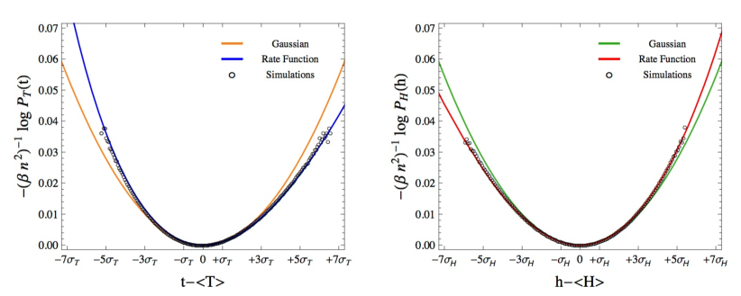
Figure 2: Numerical simulations (black circles) of complex ($\beta=2$) Wishart matrices $\mathcal{S}$ of size $n=15$ with $c=2$. Here the sample size is $N=2.5\cdot 10^{8}$. Left: The numerical values (black circles) for the total variance $T=n^{-1}\sum_{i}\lambda_{i}$. The Gaussian approximation (orange line) with average $\left<T\right>$ (15) and standard deviation $\sigma_{T}=\sqrt{\mathrm{var}(T)}$ (16) fits well the data for fluctuations of order $\sim 3\sigma_{T}$ but deviates strongly for atypical fluctuations. The global behavior is captured instead by the large deviation function (blue line) $\Psi_{T}(t)$ of (19). Right: Numerical values (black circles) for the log-determinant $H=n^{-1}\sum_{i}\ln\lambda_{i}$. Again, the Gaussian approximation (green line) with average $\left<H\right>$ (15) and standard deviation $\sigma_{H}=\sqrt{\mathrm{var}(H)}$ (16) describes well the data for fluctuations of order $\sim 3\sigma_{H}$ but deviates for larger fluctuations. The large deviation function (red line) $\Psi_{H}(h)$ of (45) provides a global description of the data. The critical point $h=-1$ (below which the large deviations change speed from $n^{2}$ to $n$) is not visible in the picture (for $n=15$ and $c=2$ the critical point is at $\sim 25\sigma_{H}$ to the left of $\left<H\right>$).

Once the joint large-$n$ behavior of generalized and total variances is known, one may easily derive a large deviation principle for any continuous function of them. For instance, from $\widehat{\mathcal{P}}(s,w)$, it is easy to compute the Laplace transform of the likelihood ratio $L=T-H-1$ as $\widehat{\mathcal{P}}_{L}(s)=\langle\rme^{-\beta n^{2}sL}\rangle=\rme^{\beta n^{2}s}\widehat{\mathcal{P}}(-s,s)$. Hence we have the following result.

B: Large deviations of the likelihood ratio.  

The likelihood ratio cumulant GF is given by

$$J_{L}(s)=-\lim_{n\to\infty}\frac{1}{\beta n^{2}}\ln\widehat{\mathcal{P}}_{L}(s)=J(-s,s)-s\qquad\text{for}\,\,\,-1/2<s\leq s_{c}\ ,$$ (21)

with $J$ as in (11). With the same notation as above, the cumulants of $L$ at leading order in $n$ follow by differentiations

$$C_{\ell}(L)=C_{\ell}(T)+(-1)^{\ell}C_{\ell}(H)+\delta C_{\ell}\quad\mathrm{with}\quad\delta C_{\ell}=\omega_{\beta}(n,\ell)\frac{\ell\,!}{(1-\ell)}\theta\left(\ell-1\right)-\delta_{\ell,1}\ ,$$ (22)

($\theta$ is the Heaviside step function) for $\ell\geq 1$. This corresponds to typical fluctuations on a region $\mathcal{O}(1/n)$ around the mean

$$\left<L\right>=c+(c-1)\ln{(c-1)}-c\ln{c},$$ (23)

with variance

$$\mathrm{var}(L)=\omega_{\beta}(n,2)\left[c+\ln{(c/(c-1))}-2\right].$$ (24)

Note that, since $T$ and $H$ are not independent, the cumulants (22) of $L$ involve the extra term $\delta C_{\ell}$.

From Result A, extracting the asymptotics of the first moments of $T$ and $H$ for $c\gg 1$ we recover classical results in multivariate analysis, valid when the sample size $m$ is much larger than the number of variates $n$.

C: Classical statistics.  

In the regime $m\gg n\gg 1$, $T$ and $H$ become asymptotically Gaussian. More precisely, as $c\to\infty$

$$\sqrt{\frac{\beta n^{2}}{2c}}\left(T-c\right)\to\mathcal{N}(0,1),\qquad\text{and}\qquad\sqrt{\frac{\beta cn^{2}}{2}}\left(H-\ln{c}\right)\to\mathcal{N}(0,1),$$ (25)

in distribution, where $\mathcal{N}(0,1)$ denotes a standard Gaussian variable.

To conclude this introductory section, we remark that our findings reproduce some known results for the typical fluctuations (mean and variance) of $T,H$ and $L$ separately, in the real case ($\beta=1$) [2, 31, 4, 32, 29]. Moreover, the variances and covariances (16) and (24) can be computed for generic $\beta$ using covariance formulae valid for one-cut $\beta$-ensembles of random matrices [6, 12].

A precious tool in classical statistics is the Barlett decomposition [5], which is useful to transform functions of strongly correlated eigenvalues of Wishart matrices (see (5)) into functions of independent (but not identical) chi-squared random variables. In the asymptotic regime $m\gg n$ this decomposition becomes sufficiently manageable to derive some interesting results. For real matrices, the limits (25) agree with classical theorems based on the Barlett decomposition (see e.g. [40]). From the results on $H$, the statistical behavior of the scaled determinant $G=\rme^{H}$ can be easily derived. For statistics of determinants of random matrices (more general than the sample covariance matrices considered here), see [10, 43, 33, 49]. For more details on the classical methods in multivariate analysis we refer to the classical books [40, 30] and the excellent review [31] on the applications of RMT in multivariate statistics.

3 Derivation

We now turn to the derivation of Result A. Results B and C follow as corollaries and hence their proof will be omitted. In Subsection 3.1 we set up the variational problem in the framework of the 2D Coulomb gas thermodynamics. The Coulomb gas analogy for spectra of random matrix ensembles goes back to the seminal works by Wigner [54] and Dyson [20]. In particular, it was Dyson who first used this analogy to compute large random matrix statistics. This idea has been developed later and used in several areas of physics [8, 9, 17, 53, 22, 18, 34, 35, 23, 50, 36, 37, 28, 13, 14, 11, 16, 15]. In Subsection 3.2 we solve the saddle-point equations and we compute explicitly $J(s,w)$, thus proving Result A.

3.1 2D Coulomb gas problem

The Coulomb gas calculation goes as follows. First we observe from (5)-(6) that the joint Laplace transform (8) is finite for $s\leq\alpha=s_{c}+\mathcal{O}\left(n^{-1}\right)$ and $w>-1/2$. From (5) and (7)-(8), this Laplace transform can be written as the ratio of two partition functions

$$\widehat{\mathcal{P}}_{n}(s,w) =\left[\mathcal{Z}_{n}(s,w)/\mathcal{Z}_{n}(0,0)\right],$$ (26)

$$\mathcal{Z}_{n}(s,w) =\int\mathrm{d}\lambda_{1}\cdots\mathrm{d}\lambda_{n}\,\rme^{-\beta E[\bm{\lambda};s,w]}\ .$$ (27)

$\mathcal{Z}_{n}(s,w)$ is the partition function of a constrained Coulomb gas, where the energy function $E[\bm{\lambda};s,w]=E[\bm{\lambda}]+\sum_{k}U_{s,w}(\lambda_{k})$ contains now the additional single-particle potential

$$U_{s,w}(\lambda)=s\ln\lambda+w\lambda\ .$$ (28)

Note that $\mathcal{Z}_{n}(0,0)$ is the partition function of the unconstrained gas and therefore it coincides with the normalization constant in (5).

Hence, the computation of the joint cumulant GF $J(s,w)$ amounts to evaluating the leading order in $n$ of the partition function $\mathcal{Z}_{n}(s,w)$. More precisely, from (26)-(27), $J(s,w)$ may be expressed as the excess free energy

$$J(s,w)=-\lim_{n\to\infty}\frac{1}{\beta n^{2}}\left[\ln\mathcal{Z}_{n}(s,w)-\ln\mathcal{Z}_{n}(0,0)\right]$$ (29)

of the Coulomb gas in the effective potential $V(\lambda)+U_{s,w}(\lambda)$ with respect to the unperturbed Coulomb gas ($s=w=0$). This effective potential is bounded from below for $s\leq\alpha=s_{c}+\mathcal{O}\left(n^{-1}\right)$ and $w>-1/2$ (the domain of existence of the Laplace transform $\widehat{\mathcal{P}}_{n}(s,w)$, of course). For any finite $n,m$, the excess free energy (29) can be computed exactly in terms of a Laguerre-Selberg integral [45] (see Section 4). How to deal with the limit of large $n$? We show now how the task of computing $J(s,w)$ can be reduced to a variational problem.

First, we introduce the normalized density of the gas particles $\rho_{n}(\lambda)=n^{-1}\sum_{i=1}^{n}\delta(\lambda-\lambda_{i})$, in terms of which any sum function on the eigenvalues $\lambda_{1},\dots,\lambda_{n}$ can be easily expressed. For instance, the log-determinant and trace (7), both linear statistics on $\mathcal{S}$, are conveniently expressed as linear functionals on $\rho_{n}(\lambda)$ as

$$H=\int\mathrm{d}\rho_{n}(\lambda)\,\ln\lambda\qquad\text{and}\qquad T=\int\mathrm{d}\rho_{n}(\lambda)\,\lambda\ .$$ (30)

Second, for large $n$, the energy function $E[\bm{\lambda};s,w]$ of the 2D Coulomb gas can be converted into a mean-field energy functional $E[\bm{\lambda};s,w]\sim n^{2}\mathcal{E}[\rho_{n};s,w]$, where

$$\mathcal{E}[\rho;s,w]=-\frac{1}{2}\iint_{\lambda\neq\lambda^{\prime}}\!\!\!\!\!\mathrm{d}\rho(\lambda)\,\mathrm{d}\rho(\lambda^{\prime})\,\ln|\lambda-\lambda^{\prime}|+\int\mathrm{d}\rho(\lambda)\,V(\lambda)+\int\mathrm{d}\rho(\lambda)\,U_{s,w}(\lambda)\ .$$ (31)

The mean-field functional (31) has been intensely studied in several fields. We refer to [44, 46, 16] for a detailed exposition and collection of known results. In particular, it is known that for large $n$ the partition function $\mathcal{Z}_{n}(s,w)$ is dominated by $\rho_{s,w}(\lambda)$, the unique minimizer of the mean-field energy functional $\mathcal{E}[\rho;s,w]$ in the space of normalized densities:

$$\mathcal{Z}_{n}(s,w)\approx\exp\left({-\beta n^{2}\mathcal{E}[\rho_{s,w};s,w]}\right)\;\;\;\text{with}\;\;\;\mathcal{E}[\rho_{s,w};s,w]=\min_{\begin{subarray}{c}\rho\geq 0\\ \int\!\mathrm{d}\rho=1\end{subarray}}\mathcal{E}[\rho;s,w]\ .$$ (32)

The meaning of the saddle-point density is the following: $\rho_{s,w}(\lambda)$ is the typical configuration of the eigenvalues yielding a prescribed value of log-determinant and trace

$$h(s,w)=\int\mathrm{d}\rho_{s,w}(\lambda)\,\ln\lambda\qquad t(s,w)=\int\mathrm{d}\rho_{s,w}(\lambda)\,\lambda\ .$$ (33)

Hence, a possible route to evaluate $J(s,w)$ consists of finding for all $s,w$ the saddle-point density $\rho_{s,w}(\lambda)$ and inserting it back into the energy functional (31) to evaluate the leading order of $\mathcal{Z}_{n}(s,w)$ as in (32). This technique has been exploited in the last decade in many physical problems, mainly to compute the large deviations of single observables. However, this route entails the explicit computation of the mean-field energy (31) at the saddle-point density, which is not necessarily an easy task. The situation gets even worse in the case of joint statistics.

In certain situations one can use a shortcut (see [16]) based on a thermodynamic identity that has been stated rigorously in the language of large deviation theory [51] by Gärtner [27] and Ellis [21]. It is known that, if a cumulant GF $J(\vec{s})$ is differentiable in the interior of its domain, then the rate function $\Psi(\vec{x})$ is the Legendre-Fenchel transform of the cumulant GF (and hence, $J(\vec{s})$ is the inverse Legendre-Fenchel transform of $\Psi(\vec{x})$). This relation between rate function and cumulant GF can be exploited in our problem as follows (for a general mathematical discussion we refer to [16]). We assume first that $J(s,w)$ is differentiable. Therefore, the Gärtner-Ellis theorem ensures that $\Psi(h,t)$ is also smooth and given from $J(s,w)$ by the Legendre-Fenchel transformation

$$\Psi(h,t)=\sup_{s,w}\left[J(s,w)-(sh+wt)\right]\ .$$ (34)

The identity (34) can be written in the (almost) symmetric form

$$J(s,w)-\Psi(h,t)=sh+wt\ .$$ (35)

This equation should be interpreted with care. Indeed, in (35), there are only two independent variables, for instance $s$ and $w$ or $h$ and $t$. The relation between the conjugate variables $(h,t)$ and $(s,w)$ is provided by

$$\frac{\partial J(s,w)}{\partial s}=h(s,w)\,,\frac{\partial J(s,w)}{\partial w}=t(s,w)\quad\text{or equivalently}\quad\frac{\partial\Psi(h,t)}{\partial h}=s(h,t)\,,\frac{\partial\Psi(h,t)}{\partial h}=w(h,t)\ ,$$ (36)

where $h(s,w)$ and $t(s,w)$ are given in (33) and $s(h,t)$, $w(h,t)$ are the corresponding inverse maps. Hence, we can write the differential relations

$$\mathrm{d}J(s,w) =h(s,w)\mathrm{d}s+t(s,w)\mathrm{d}w$$ (37)

$$-\mathrm{d}\Psi(h,t) =s(h,t)\mathrm{d}h+w(h,t)\mathrm{d}t\ ,$$ (38)

supplemented with the normalization condition $J(0,0)=0$ (and hence $\Psi(h(0,0),t(0,0))=0$). The expressions (37) and (38) can be interpreted as Maxwell relations among thermodynamic potentials, in our case the Helmholtz free energy and the enthalpy. However it is somewhat astonishing that these relations have not been applied in the Coulomb gas computations until very recently (for applications of (37)-(38) in physical models see [13, 14] and also [28]).

Using (37)-(38) one can use the following shortcut to compute the large deviations functions (for a detailed exposition we refer to [16]). For instance, in order to compute $J(s,w)$ we only need to find the saddle-point density $\rho_{s,w}(\lambda)$ and compute $h(s,w)$ and $t(s,w)$ from (33). Then, $J(s,w)$ follows from integration of (37)

$$J(s,w)=\int_{(0,0)}^{(s,w)}\!\mathrm{d}J(s,w)\ .$$ (39)

This shortened route of the Coulomb gas method provides an effective tool to evaluate large deviations functions. A large amount of unnecessary computations can be avoided and the task of computing joint large deviations becomes feasible. In the next subsection, we will use this strategy to derive our main result.

3.2 Saddle-point equation and large deviation functions

The first problem to overcome is to find the saddle-point density $\rho_{s,w}$ of the mean-field functional $\mathcal{E}[\rho;s,w]$. From (31), the stationarity condition of $\rho_{s,w}$ reads

$$\int\mathrm{d}\rho_{s,w}(\lambda^{\prime})\,\ln|\lambda-\lambda^{\prime}|-V(\lambda)-U_{s,w}(\lambda)=\mathrm{const},\,\qquad\text{for}\,\,\lambda\in\operatorname{supp}\rho_{s,w},$$ (40)

where $\operatorname{supp}\rho_{s,w}$ denote the support of $\rho_{s,w}$ (for $\lambda\notin\operatorname{supp}\rho_{s,w}$ the left hand side is greater than or equal to the same constant). The physical meaning of (40) is clear: at equilibrium, the 2D Coulomb gas arranges itself in such a way that each particle has equal electrostatic energy (the left hand side of (40)).

Taking one further derivative with respect to $\lambda$, the resulting singular integral equation can be solved for $\rho_{s,w}(\lambda)$ using a theorem due to Tricomi ([52, Sec. 4.3]), and the result reads

$$\rho_{s,w}(\lambda)=\frac{1+2w}{2\pi\lambda}\sqrt{\left(\lambda-\lambda_{-}\right)\left(\lambda_{+}-\lambda\right)}\,{\bm{1}}_{\lambda\in(\lambda_{-},\lambda_{+})},$$ (41)

where the edges $\lambda_{\pm}$ of the support depend on $s$ and $w$ as

$$\lambda_{\pm}(s,w)=\frac{1}{1+2w}\left(1\pm\sqrt{1-2\left(s-s_{c}\right)}\right)^{2}.$$ (42)

For $s=w=0$ the density of the unperturbed gas $\rho_{0,0}(\lambda)$ coincides with the Marčenko-Pastur distribution [38] with edges $(1\pm\sqrt{c})^{2}$. For $s<s_{c}$ the saddle-point density is bounded while at $s=s_{c}$ the lower edge $\lambda_{-}(s_{c},w)=0$ reaches the origin and $\rho_{s,w}$ acquires an inverse square root divergence there.

From $\rho_{s,w}$ the corresponding values of scaled log-determinant $H$ and trace $T$ are

$$\begin{cases}\displaystyle h(s,w)=\int\mathrm{d}\rho_{s,w}(\lambda)\,\ln\lambda=\varphi\left(s-s_{c}\right)-\ln(1+2w)\\ \displaystyle t(s,w)=\int\mathrm{d}\rho_{s,w}(\lambda)\,\lambda=\displaystyle\frac{c-2s}{1+2w}\ ,\end{cases}$$ (43)

with $\varphi(x)=-1+(1-2x)\ln{\left(1-2x\right)}+2x\ln{(-2x)}$ for $x\leq 0$ (hence $h(s,w)$ is defined for $s\leq s_{c}$). Combining (43) and (39) we obtain the cumulant GF $J(s,w)$ as in Result A.

In principle, one may also compute the rate function $\Psi(h,t)$ in the same way. However, it is not possible to write down $s(h,t)$ and $w(h,t)$ (the inverse maps of (43)) in terms of elementary functions. For simplicity, however, we show how to carry out the explicit computation for trace and log-determinant separately and establish the large $n$ decay as in Remark 4. Setting $s=0$ we find $t(0,w)=c/(1+2w)$ from (43), and we immediately get the rate function of the scaled traces from (39) by integrating $w(t)$ (the inverse of $t(0,w)$)

$$\Psi_{T}(t)=-\int_{t(0,0)}^{t}{w(t^{\prime})\mathrm{d}t^{\prime}}=\int_{c}^{t}{\frac{1}{2}\left(1-\frac{c}{t^{\prime}}\right)\mathrm{d}t^{\prime}}=\frac{t-c}{2}+\frac{c}{2}\ln{\left(\frac{c}{t}\right)}.$$ (44)

This proves (19). Similarly, for the log-determinant $H$ we have

$$\Psi_{H}(h)=-\int_{h(0,0)}^{h}s(h^{\prime})\mathrm{d}h^{\prime},$$ (45)

valid for $h>-1$ (see discussion in the next Section), where $s(h)$ is the inverse of $h(s,0)$.

4 Further results and discussion

The treatment in the previous section does not cover the following two issues:

• The case $c=1$ (square data matrices), for which the leading term of the variance of $H=\ln\det\mathcal{S}$ (computed from the approach described above) is not defined (see Eq. (16)). What is the origin of this hitch?

• The origin of the condition $h>-1$ for the validity of the rate function $\Psi_{H}(h)$ in (45) seems mysterious. What is the mechanism governing the statistics of “anomalously small" log-determinants, then?

We discuss these two issues in detail here.

4.1 The case $c=1$ (square data matrices)

As already disclosed, if $\mathcal{S}$ is a Wishart matrix with $c=1$ ($m=n$) the limiting variance of $H=\ln\det\mathcal{S}$ is not described by our large deviations result (see Eq. (16)). The origin of this hitch is as follows. Recall that the cumulant GF $J_{H}(s)$ is defined for $s\leq s_{c}=(c-1)/2$. Hence, for $c=1$ (i.e. $m=n$) $J_{H}(s)$ is non-analytic in $s=s_{c}=0$ and the cumulants cannot be obtained by differentiation.

A way to circumvent this problem is to first compute $\mathrm{var}(H)$ for finite $n$, and then evaluate its large $n$ asymptotics. The joint Laplace transform $\widehat{\mathcal{P}}_{n}(s,w)$ of $H$ and $T$ can be indeed evaluated exactly also at finite $n,m$, using the Laguerre-Selberg integral [45, 26, 3]:

$$\frac{1}{n!}\int_{0}^{+\infty}\cdots\int_{0}^{+\infty}\prod_{i<j}|x_{i}-x_{j}|^{2p}\prod_{i=1}^{n}x_{i}^{q-1}\rme^{-x_{i}}\mathrm{d}x_{i}=\prod_{j=0}^{n-1}\frac{\Gamma(q+jp)\Gamma\left((j+1)p\right)}{\Gamma(p)},\qquad p,q>0\ .$$ (46)

Using this identity, one may evaluate the Laplace transform $\widehat{\mathcal{P}}_{n}(s,w)$ as

$$\widehat{\mathcal{P}}_{n}(s,w)=\left(\frac{(\beta n/2)^{s}}{\left(2w+1\right)^{\frac{1}{2}+(\alpha-s)+\frac{1}{2n}}}\right)^{\beta n^{2}}\,\,\prod_{j=0}^{n-1}{\frac{\Gamma\left(\frac{\beta}{2}\left(j+2n(\alpha-s)\right)+1\right)}{\Gamma\left(\frac{\beta}{2}\left(j+2n\alpha\right)+1\right)}}\ ,$$ (47)

with $\alpha$ as in (6). We have verified that our large $n$ formulae reproduce with good accuracy the finite $n,m$ result even for moderate values of $n$.

From (47) it is possible to extract the large deviation functions for the scaled trace $T$ (this corresponds to $s=0$). On the other hand, the asymptotic in the variable $s$ is not trivial.

However we can use this exact result to deduce $\mathrm{var}(H)$ for symmetric data matrices ($c=1$), the case that was not covered by our Result A. Setting $c=1$ and $w=0$ in (47), we denote by $\widehat{\mathcal{P}}_{n}(s)\equiv\widehat{\mathcal{P}}_{n}(s,0)=\langle\rme^{-\beta n^{2}sH}\rangle$ the Laplace transform of $H$ at finite $n=m$. We can compute the derivatives of $\widehat{\mathcal{P}}_{n}(s)$ as

$$\widehat{P}_{n}^{\prime}(s) =\beta n^{2}\ln\left(\frac{\beta n}{2}\right)\ \widehat{P}_{n}(s)-\beta n\widehat{P}_{n}(s)\sum_{j=0}^{n-1}\psi_{0}\left(\frac{\beta}{2}(j+1-2ns)\right)\ ,$$ (48)

$$\widehat{P}_{n}^{\prime\prime}(s) =\beta n^{2}\ln\left(\frac{\beta n}{2}\right)\widehat{P}_{n}^{\prime}(s)-\beta n\widehat{P}_{n}^{\prime}(s)\sum_{j=0}^{n-1}\psi_{0}\left(\frac{\beta}{2}(j+1-2ns)\right)$$

$$+(\beta n)^{2}\widehat{P}_{n}(s)\sum_{j=0}^{n-1}\psi_{1}\left(\frac{\beta}{2}(j+1-2ns)\right)\ ,$$ (49)

where $\psi_{m}(z)=\partial_{z}^{m+1}\ln\Gamma(z)$ is the $m$-Polygamma function [1]. In principle one can compute higher derivatives recursively, and evaluate the asymptotic values of the cumulants of $H$. For instance, average and variance of $H$ are related to the derivatives $\widehat{P}_{n}^{\prime}(s)$ and $\widehat{P}_{n}^{\prime\prime}(s)$ at $s=0$. Using the normalization $\widehat{P}_{n}(0)=1$ we get

$$\langle H\rangle =-\frac{1}{\beta n^{2}}\widehat{P}_{n}^{\prime}(0)=-\ln\left(\frac{\beta n}{2}\right)+\frac{1}{n}\sum_{j=0}^{n-1}\psi_{0}\left(\frac{\beta}{2}(j+1)\right)\ .$$ (50)

Using the Euler-Maclaurin summation formula [1] $\sum_{k=0}^{N}F(a+hk)=\frac{1}{h}\int_{a}^{b}\mathrm{d}t\,F(t)+\frac{1}{2}\left[F(b)+F(a)\right]+\dots$ (with $b=a+hN$), and the classical asymptotic $\ln\Gamma(az+b)\sim\ln(\sqrt{2\pi})-az+\left(az+b-\frac{1}{2}\right)\ln(az)$, valid for $z\to\infty$, with $|\arg z|<\pi$ and $a>0$, we obtain for large $n$ the limit value $\langle H\rangle\to-1$, according to (15) for $c=1$. A similar analysis of the Laguerre-Selberg integral (for $w=0$) was performed in [10], but it was restricted to the computation of $\left<H\right>$ at leading order in $n$. Here we tackle the problem of the variance of $H$ for square data matrices. From (49) we obtain

$$\mathrm{var}(H)=\langle H^{2}\rangle-\langle H\rangle^{2}=\frac{1}{(\beta n^{2})^{2}}\left\{\widehat{P}_{n}^{\prime\prime}(0)-\widehat{P}_{n}^{\prime}(0)^{2}\right\}=\frac{1}{n^{2}}\sum_{j=0}^{n-1}\psi_{1}\left(\frac{\beta}{2}(j+1)\right)\ .$$ (51)

After a somewhat lengthy calculation, we managed to extract the large $n$ asymptotics

$$\frac{\mathrm{var}(H)}{\omega_{\beta}(n,2)}=\ln n+\ln(\beta/2)-\psi_{0}(\beta/2)+1+K_{\beta}+o(1)\ ,$$ (52)

with a constant $K_{\beta}$ given by

$$K_{\beta}=(2/\beta^{2})\int_{0}^{\infty}t\,\rme^{-2t(1-1/\beta)}(\beta\rme^{2t/\beta}-2\rme^{t}+2-\beta)(1-\rme^{-t})^{-1}(\rme^{2t/\beta}-1)^{-2}\mathrm{d}t\ .$$ (53)

Some special values are $K_{1}=\pi^{2}/8-\ln 2,K_{2}=0,K_{4}=1-\pi^{2}/8$. This result has been verified numerically, see Fig. 3. Note the logarithmic growth of (52) with $n$, in contrast to the $\mathcal{O}(1)$ limiting behavior of $\mathrm{var}(H)/\omega_{\beta}(n,2)$ for $c>1$. Such a logarithmic divergent variance is customary for discontinuous spectral linear statistics in RMT, the paradigmatic example being the number variance [20, 34, 36, 39]. Notice that the function $\ln\lambda$ is indeed discontinuous at $\lambda=0$. However, as long as $s<s_{c}$ the support of the equilibrium measure $\rho_{s,w}(\lambda)$ does not contain the origin and this singularity is ineffective; only for $s=s_{c}$ we have $\lambda_{-}(s_{c},w)=0$, and at that point the singularity of $\ln\lambda$ starts being felt. The central limit theorem with logarithmically divergent variance for $H$ has been proved in [42, 41] for $\beta=1$. The subleading corrections to $\mathrm{var}(H)$ in (52) are instead a new result.

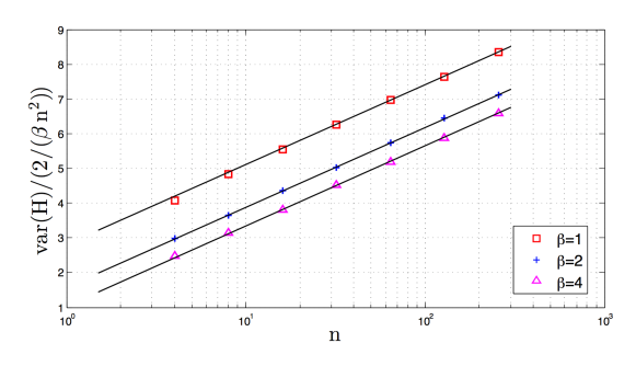
Figure 3: Rescaled variance of the log-determinant $H=n^{-1}\sum_{i}\ln(\lambda_{i})$ for $c=1$. Each point is produced sampling $N=10^{6}$ Wishart matrices of size $n$ for $\beta=1,2$ and $4$. The error for each point is of order $\mathcal{O}(10^{-2})$, not visible in the picture. The solid lines are the exact result (52).

4.2 The statistics of atypically small log-determinants

We have claimed earlier that the rate function $\Psi_{H}(h)$ of $H$ can be computed as the inverse Legendre-Fenchel transform of $J_{H}(s)$ only for $h>-1$. Why is this the case? As a matter of fact, the Gärtner-Ellis theorem has two hypotheses: first, the cumulant GF is required to be differentiable in the interior of its domain; second, the derivatives of the cumulant GF should diverge on the boundaries of the domain (a condition known as steepness [21, 51]). In our case, $J_{H}(s)$ is differentiable for all $s<s_{c}$ but the left derivative attains a finite value at the boundary point $s_{c}$: $\partial_{s}J_{H}(s)\to-1$ as $s\to s_{c}^{-}$. Hence, only a local version of the Gärtner-Ellis theorem holds and $\mathcal{P}_{H}(h)\approx\exp(-\beta n^{2}\Psi_{H}(h))$ with $\Psi_{H}(h)$ being the branch of the Legendre-Fenchel transform of $J_{H}(s)$ for $h>-1$.

The 2D Coulomb gas analogy provides a rather intuitive physical picture of this obstruction. We have seen that the saddle-point density $\rho_{s,w}$ is bounded as long as $s<s_{c}$ (see (41)-(42)). When $s=s_{c}$, the lower edge of the saddle-point density reaches the origin $\lambda_{-}(s_{c},w)=0$ and $\rho_{s_{c},w}(\lambda)\sim\lambda^{-1/2}$ acquires an inverse square-root singularity there. For $s>s_{c}$, the logarithmic part of the effective potential $V(\lambda)+U_{s,w}(\lambda)$ becomes attractive, giving rise to an electrostatic instability of the gas. As already discussed, $\rho_{s,w}(\lambda)$ is the typical distribution of the eigenvalues of $\mathcal{S}$ yielding a prescribed value of $H=\int\mathrm{d}\rho_{s,w}(\lambda)\,\ln\lambda$. Setting $w=\alpha=0$ to simplify the discussion, we see that $\int\mathrm{d}\rho_{s,0}(\lambda)\,\ln\lambda>-1$ as long as $s<s_{c}$ and the critical value $H_{\text{cr}}=-1$ corresponds to the critical density $\rho_{s_{c},0}(\lambda)=\frac{1}{2\pi}\sqrt{(4-\lambda)/\lambda}\,{\bm{1}}_{\lambda\in(0,4)}$ obeying $\int\mathrm{d}\rho_{s_{c},0}(\lambda)\,\ln\lambda=H_{\text{cr}}$. A solution to the problem of smaller log-determinant $H<H_{\text{cr}}$ would be achieved if the typical distribution of the eigenvalues corresponding to this anomalously small $H$ were known.

What is then the behavior of the Coulomb gas constrained to have $H<H_{\text{cr}}$? As suggested in [16], a failure of the steepness condition may be the hallmark of split-off phenomena of random variables. Guided by numerics and intuition, since the function $\ln\lambda$ is divergent for $\lambda\downarrow 0$, we expect that atypically small values of $H=n^{-1}\sum_{i=1}^{n}\ln\lambda_{i}<H_{\text{cr}}$ are driven by the statistical behavior of the smallest eigenvalue $\lambda_{\min}$. For $H>H_{\text{cr}}$ the Coulomb gas particles behave ‘cooperatively’ to accommodate atypical values of $H$ (each of the random variables $\ln\lambda_{i}$’s contributes to realize $H$). On the contrary, large fluctuations of $H<H_{\text{cr}}$ are typically realized by fluctuations of $\lambda_{\min}$ to the left (the random variable $\ln\lambda_{\min}$ contributes macroscopically to $H$). This line of reasoning would imply a change of scaling (speed) in the large $n$ behavior of the probability density of $H$. The idea is to split the contribution of the Coulomb gas to $H$ in two parts:

$$H[\rho]=\frac{1}{n}\ln\lambda_{\mathrm{min}}+H[\tilde{\rho}]\ ,\quad\text{where}\quad\tilde{\rho}(\lambda)=\frac{1}{n}\sum_{i:\lambda_{i}\neq\lambda_{\mathrm{min}}}\delta(\lambda-\lambda_{i})\ .$$ (54)

The probability density of $H$ can be written as

$$\mathcal{P}_{H}(h)=\int_{0}^{+\infty}\mathrm{d}x\mathcal{P}_{H}\left(h\,|\,\lambda_{\mathrm{min}}=x\right)\mathcal{P}_{\lambda_{\mathrm{min}}}(x)\ .$$ (55)

At this point we need to understand the distribution of the smallest eigenvalue $\mathcal{P}_{\lambda_{\mathrm{min}}}(x)$ and the conditional probability $\mathcal{P}_{H}\left(h\,|\,\lambda_{\mathrm{min}}=x\right)$. It is easy to show that the probability density function of the smallest eigenvalue behaves for large $n$ as

$$\mathcal{P}_{\lambda_{\mathrm{min}}}(x)\approx\mathrm{e}^{-\beta n^{2}x/2}\ ,$$ (56)

corresponding to a typical value $\left<\lambda_{\mathrm{min}}\right>=2/(\beta n^{2})$ and $\mathrm{var}(\lambda_{\mathrm{min}})=4/(\beta^{2}n^{4})$ at leading order in $n$. Typical fluctuations of order $\mathcal{O}(n^{-2})$ to the right of $\left<\lambda_{\mathrm{min}}\right>$ are irrelevant for the statistical behavior of $H$. On the contrary the typical fluctuations to the left ($\lambda_{\mathrm{min}}<\left<\lambda_{\mathrm{min}}\right>$) play a significant role due to the divergent character of $\ln\lambda_{\mathrm{min}}$ for $\lambda_{\mathrm{min}}\downarrow 0$. Roughly speaking, the typical fluctuations of order $\mathcal{O}(n^{-2})$ of the smallest eigenvalues do not change the limiting macroscopic density of the eigenvalues ($\tilde{\rho}(\lambda)\simeq\rho_{s_{c},0}(\lambda)$, irrespective of the value of $H\leq H_{\mathrm{crit}}$), but nevertheless have dramatic consequences on the statistics of $H$.

Similar evaporation phenomena for both correlated and i.i.d. variables have been recently detected in a variety of contexts (see e.g. [18, 50, 24, 48, 53, 7, 23]). The new interesting twist here is that the split-off is realized by the smallest (and not the usual largest) of the random variables involved. Here, using $H\left[\tilde{\rho}\right]\simeq H\left[{\rho_{s_{c},0}}\right]=-1$, for $0\leq x\leq\left<\lambda_{\mathrm{min}}\right>$ we have:

$$\mathcal{P}_{H}\left(h\,|\,\lambda_{\mathrm{min}}=x\right) =\mathcal{P}_{H}\left(h=\frac{1}{n}\ln\lambda_{\mathrm{min}}+H\left[\tilde{\rho}\right]\,\bigg{|}\,\lambda_{\mathrm{min}}=x\right) \rightarrow\delta\left(h-\left(\frac{1}{n}\ln\lambda_{\mathrm{min}}-1\right)\right)\ .$$ (57)

Using the above result, from (55), we easily get

$$\mathcal{P}_{H}(h)\approx\mathrm{e}^{-n\tilde{\psi}_{H}(h)},\quad\text{with}\quad\tilde{\psi}_{H}(h)=-1-h\ ,$$ (58)

for $h<-1$ (note the speed $n$ in contrast to the speed $n^{2}$ in the “democratic" Coulomb gas setting).

A further argument in support of this change of speed can be obtained for $\beta=2$ and $\alpha=0$ using a finite-$n$ approach based on the Laguerre-Selberg integral (46). It is convenient to work directly at the level of the determinant of $\mathcal{S}$. Let $\mathcal{P}_{\hat{G}}(\hat{g})$ be the probability density of the determinant $\hat{G}=\det(\mathcal{S})=\prod_{i=1}^{n}\lambda_{i}$ (without the power $1/n$). Its Mellin transform is given by

$$\hat{M}(\hat{s})=\int_{0}^{\infty}\mathrm{d}\hat{g}\mathcal{P}_{\hat{G}}(\hat{g})\hat{g}^{\hat{s}-1}=\left(\frac{1}{n}\right)^{n(\hat{s}-1)}\frac{G(n+\hat{s})\Gamma(\hat{s})}{G(n+1)G(1+\hat{s})}\ ,$$ (59)

where $G(x)$ is the Barnes G-function. Using the asymptotics [1]

$$\frac{G(n+\hat{s})}{G(n+1)}\sim\exp\left[n(1-\hat{s})-n\ln n+\hat{s}\ n\ln n+\ln n[1/2-\hat{s}+\hat{s}^{2}/2]-\ln(2\pi)(1-\hat{s})/2+o(1/n)\right],$$ (60)

valid for $n\to\infty$, we obtain (with logarithmic accuracy)

$$\hat{M}(\hat{s})\approx\rme^{-n(\hat{s}-1)}\ .$$ (61)

This Mellin transform can be written also in terms of the probability density $\mathcal{P}_{H}(h)$ of $H=n^{-1}\ln\hat{G}$. Assuming $\mathcal{P}_{H}(h)\approx\rme^{-n\tilde{\psi}_{H}(h)}$ for $h<-1$ we have

$$\hat{M}(\hat{s})=\int_{-\infty}^{\infty}\mathrm{d}h\mathcal{P}_{H}(h)e^{n(\hat{s}-1)h}\approx\int_{-\infty}^{-1}\mathrm{d}h\ \rme^{-n\left[\tilde{\psi}_{H}(h)-(\hat{s}-1)h\right]}\approx\exp\left[-n\min_{h}\left(\tilde{\psi}_{H}(h)-(\hat{s}-1)h\right)\right]\ .$$ (62)

Here the integral has been truncated at $h=-1$ since $\mathcal{P}_{H}(h)$ decays faster (exponentially with speed $n^{2}$) for $h>-1$, and Laplace’s approximation has been used in the last step. Matching (61) with (62), we eventually obtain $\tilde{\psi}_{H}(h)$ as in (58).

5 Conclusions

In summary, we have considered the joint statistics (including large deviation tails) of generalized and total variance of a large $n\times m$ Gaussian dataset. These observables are just the scaled log-determinant $H$ and the trace $T$ of the corresponding $n\times n$ covariance matrix. We have employed a powerful combination of two techniques: the Coulomb gas analogy of statistical physics, which allowed us to represent the eigenvalues of the covariance matrix as an interacting gas of charged particles, whose excess free energy is the the cumulant generating function for our observables in the limit $n,m\to\infty$ with $c=m/n$ fixed, and a finite $n,m$ approach based on the Laguerre-Selberg integral. Combining these two approaches, we complemented the Coulomb gas method with two interesting cases that fell out of its domain: i) the case $c=1$ (square datasets), for which the excess free energy is non-analytic in zero. This has the consequence that the variance of H grows logarithmically with $n$, with a subleading constant term that we could precisely characterize, and ii) atypically small log-determinants, for which the corresponding rate function in Laplace space is non-steep. This implies an abrupt change of speed in the corresponding large deviation principle, which can be ascribed to the split-off of the smallest eigenvalue from the unperturbed Marčenko-Pastur distribution. This picture is supported by numerical simulations and a saddle-point argument based on a finite $n,m$ formula (see Subsection 4.2).

It would be interesting to investigate whether our results could be extended to non-Gaussian and possibly correlated data matrices. Our derivation strongly relied on the data being normally distributed and a different approach seems to be needed for more general covariance matrices.

References

- [1] M. Abramowitz and I. A. Stegun, Handbook of mathematical functions with Formulas, Graphs, and Mathematical Tables, tenth printing, New York: Dover Publications (1972).
- [2] T. W. Anderson, An Introduction to Multivariate Statistical Analysis, Vol. 114 of Wiley Series in Probability and Statistics (Wiley, 1984).
- [3] G. W. Anderson, A. Guionnet, and O. Zeitouni, An Introduction to Random Matrices, 3rd Ed., (Cambridge University Press, 2009).
- [4] Z. B. Bai and J. W. Silverstein, CLT for linear spectral statistics of large-dimensional sample covariance matrices, The Annals of Probability 32, 1A (2004).
- [5] M. S. Barlett, On the theory of statistical regression, Proc. R. Soc. Edinb. 53, 260-283 (1933).
- [6] C. W. J. Beenakker, Universality of Brézin and Zee’s spectral correlator, Nucl. Phys. B 422, 515 (1994).
- [7] L. Bogacz, Z. Burda, W. Janke, and B. Wacław, Balls-in-boxes condensation on networks, Chaos 17, 026112 (2007).
- [8] E. Brézin, C. Itzykson, G. Parisi, and J. B. Zuber, Planar Diagrams, Commun. Math. Phys. 59, 35 (1978).
- [9] Y. Chen and S. M. Manning, Asymptotic level spacing of the Laguerre ensemble: a Coulomb fluid approach, J. Phys. A: Math. Theor. 27, 3615-3620 (1994); Some eigenvalue distribution functions of the Laguerre ensemble, J. Phys. A: Math. Gen. 29, 7561-7579 (1996).
- [10] G. M. Cicuta and M. L. Mehta, Probability density of determinants of random matrices, J. Phys. A: Math. Gen. 33, 8029 (2000).
- [11] F. Colomo and A. G. Pronko, Third-order phase transition in random tilings, Phys. Rev. E 88, 042125 (2013).
- [12] F. D. Cunden and P. Vivo, Universal covariance formula for linear statistics on random matrices, Phys. Rev. Lett. 113, 070202 (2014).
- [13] F. D. Cunden, P. Facchi, and P. Vivo, Joint statistics of quantum transport in chaotic cavities, EPL 110, 50002 (2015).
- [14] F. D. Cunden, A. Maltsev, and F. Mezzadri, Fluctuations in the 2D one-component plasma and associated fourth-order phase transition, Phys. Rev. E 91, 060105(R) (2015).
- [15] F. D. Cunden, F. Mezzadri, and P. Vivo, A unified fluctuation formula for one-cut -ensembles of random matrices, J. Phys. A: Math. Theor. 48, 315204 (2015).
- [16] F. D. Cunden, P. Facchi, and P. Vivo, A shortcut through the Coulomb gas method for spectral linear statistics on random matrices, J. Phys. A: Math. Theor. 49, 135202 (2016).
- [17] D. S. Dean and S. N. Majumdar, Large Deviations of Extreme Eigenvalues of Random Matrices, Phys. Rev. Lett. 97, 160201 (2006); Extreme value statistics of eigenvalues of Gaussian random matrices, Phys. Rev. E 77, 041108 (2008).
- [18] A. De Pasquale, P. Facchi, G. Parisi, S. Pascazio, and A. Scardicchio, Phase transitions and metastability in the distribution of the bipartite entanglement of a large quantum system, Phys. Rev. A 81, 052324 (2010).
- [19] I. Dumitriu and A. Edelman, Matrix models for beta ensembles, J. Math. Phys. 43, 5830 (2002).
- [20] F. J. Dyson, Statistical Theory of the Energy Levels of Complex Systems, J. Math. Phys. 3, 140 (1962); 3, 157 (1962); 3, 166 (1962); 3, 1191 (1962); 3, 1199 (1962).
- [21] R. S. Ellis, Large deviations for a general class of random vectors, Ann. Probab. 12 (1), 1-2 (1984) ; The theory of large deviations: from Boltzmann’s 1877 calculation to equilibrium macrostates in 2D turbulence, Physica D 133, 106-136 (1999).
- [22] P. Facchi, U. Marzolino, G. Parisi, S. Pascazio, and A. Scardicchio, Phase Transitions of Bipartite Entanglement, Phys. Rev. Lett. 101, 050502 (2008).
- [23] P. Facchi, G. Florio, G. Parisi, S. Pascazio, and K. Yuasa, Entropy-driven phase transitions of entanglement, Phys. Rev. A 87, 052324 (2013).
- [24] M. Filiasi, G. Livan, M. Marsili, M. Peressi, E. Vesselli, and E. Zarinelli, On the concentration of large deviations for fat tailed distributions, with application to financial data, Journal of Statistical Mechanics: Theory and Experiment, P09030 (2014).
- [25] R. A. Fisher, Frequency distribution of the values of the correlation coefficient in samples from an indefinitely large population, Biometrika 10, 507-521 (1915).
- [26] P. J. Forrester and S. O. Warnaar, The importance of the Selberg integral, Bull. Amer. Math. Soc. (N.S.) 45, 489 (2008).
- [27] J. Gärtner, On large deviations from the invariant measure, Theory Probab. Appl. 22, 24-39 (1977).
- [28] A. Grabsch and C. Texier, Capacitance and charge relaxation resistance of chaotic cavities —Joint distribution of two linear statistics in the Laguerre ensemble of random matrices, EPL 109, 50004 (2015); Distribution of spectral linear statistics on random matrices beyond the large deviation function – Wigner time delay in multichannel disordered wires, Preprint [arXiv:1602.03370] (2016).
- [29] D. Jiang, T. Jiang, and F. Yang, Likelihood Ratio Tests for Covariance Matrices of High-Dimensional Normal Distributions, Journal of Statistical Planning and Inference 142, 2241 (2012).
- [30] R. A. Johnsson and D. W. Wichern, Applied multivariate statistical analysis, (Prentice Hall, 2007).
- [31] I. M. Johnstone, High dimensional statistical inference and random matrices, Proc. International Congress of Mathematicians (2006), Preprint [arXiv:math/0611589 [math.ST]] (2006).
- [32] D. Jonsson, Some Limit Theorems for the Eigenvalues of a Sample Covariance Matrix, Journal of Multivariate Analysis 12, 1 (1982).
- [33] G. Le Caër and R. Delannay, The fixed-trace -Hermite ensemble of random matrices and the low temperature distribution of the determinant of an -Hermite matrix, J. Phys. A: Math. Theor. 40, 1561 (2007).
- [34] S. N. Majumdar, C. Nadal, A. Scardicchio, and P. Vivo, Index distribution of Gaussian Random Matrices, Phys. Rev. Lett. 103, 220603 (2009); How many eigenvalues of a Gaussian random matrix are positive?, Phys. Rev. E 83, 041105 (2011).
- [35] S. N. Majumdar and P. Vivo, Number of Relevant Directions in Principal Component Analysis and Wishart Random Matrices, Phys. Rev. Lett. 108, 200601 (2012).
- [36] S. N. Majumdar, G. Schehr, D. Villamaina, and P. Vivo, Large deviations of the top eigenvalue of large Cauchy random matrices, J. Phys. A: Math. Theor. 46, 022001 (2013).
- [37] S. N. Majumdar and G. Schehr, Top eigenvalue of a random matrix: large deviations and third order phase transition, J. Stat. Mech. P01012 (2014).
- [38] V. A. Marčenko and L. A. Pastur, Distribution of eigenvalues for some sets of random matrices, Math. USSR-Sb. 1, 457 (1967).
- [39] R. Marino, S. N. Majumdar, G. Schehr and P. Vivo, Number statistics for -ensembles of random matrices: applications to trapped fermions at zero temperature, Preprint [arXiv:1601.03178] (2016).
- [40] R. J. Muirhead, Aspect of multivariate statistical theory, John Wiley Sons, (2005).
- [41] H. H. Nguyen and V. Ve, Random matrices: law of the determinant, Ann. Probab. 42, 146-167 (2014).
- [42] G. Rempała and J.Wesołowski, Asymptotics for products of independent sums with an application to Wishart determinants, Statist. Probab. Lett. 74, 129–138 (2005).
- [43] A. Rouault, Pathwise asymptotic behavior of random determinants in the uniform Gram and Wishart ensembles, Preprint [arXiv:math/0509021] (2005) ; Asymptotic behavior of random determinants in the Laguerre, Gram and Jacobi ensembles, Alea 3, 181-230 (2007).
- [44] E. B. Saff and V. Totik, Logarithmic Potentials with External Fields, Springer-Verlag Berlin Heidelberg GmbH (1991).
- [45] A. Selberg, On the zeros of Riemann’s zeta-function, Skr. Norske Vid. Akad. Oslo I. 10, 1 (1942).
- [46] S. Serfaty, Coulomb Gases and Ginzburg-Landau Vortices, Courant Institute of Mathematical Sciences, New York, NY (2014); Ginzburg-Landau Vortices, Coulomb Gases, and Renormalized Energies, J. Stat. Phys. 154, 660-680 (2014).
- [47] J. W. Silverstein, The Smallest Eigenvalue of a Large Dimensional Wishart Matrix, Ann. Probab. 13 (4), 1364-1368 (1985).
- [48] J. Szavits-Nossan, M. R. Evans, and S. N. Majumdar, Constraint-driven condensation in large fluctuations of linear statistics, Phys. Rev. Lett. 112, 020602 (2014).
- [49] T. Tao and V. Vu, A central limit theorem for the determinant of a Wigner matrix, Adv. Math. 231, 74–101 (2012).
- [50] C. Texier and S. N. Majumdar, Wigner time-delay distribution in chaotic cavities and freezing transition, Phys. Rev. Lett. 110, 250602 (2013) ; ibid 112, 139902(E) (2014).
- [51] H. Touchette, The large deviation approach to statistical mechanics, Phys. Rep. 478, 1 (2009).
- [52] F. G. Tricomi, Integral Equations, Pure Appl. Math V, Interscience, London (1957).
- [53] P. Vivo, S. N. Majumdar, and O. Bohigas, Large deviations of the maximum eigenvalue in Wishart random matrices, J. Phys. A: Math. Theor. 40, 4317–4337 (2007) ; Distributions of Conductance and Shot Noise and Associated Phase Transitions, Phys. Rev. Lett. 101(21), 216809 (2008); Probability distributions of linear statistics in chaotic cavities and associated phase transitions, Phys. Rev. B 81, 104202 (2010).
- [54] E. P. Wigner, Statistical properties of real symmetric matrices with many dimensions, Canadian Mathematical Congress Proceedings (University of Toronto Press, Toronto), 174-184 (1957).
- [55] J. Wishart, The Generalised Product Moment Distribution in Samples from a Normal Multivariate Population, Biometrika 20A, 32 (1928).