Effects of tilting the magnetic field in 1D Majorana nanowires

Abstract

We investigate the effects that a tilting of the magnetic field from the parallel direction has on the states of a 1D Majorana nanowire. Particularly, we focus on the conditions for the existence of Majorana zero modes, uncovering an analytical relation (the sine rule) between the field orientation relative to the wire, its magnitude and the superconducting parameter of the material. The study is then extended to junctions of nanowires, treated as magnetically inhomogeneous straight nanowires composed of two homogeneous arms. It is shown that their spectrum can be explained in terms of the spectra of two independent arms. Finally, we investigate how the localization of the Majorana mode is transferred from the magnetic interface at the corner of the junction to the end of the nanowire when increasing the arm length.

I Introduction

In 2003 Kitaev pointed out the usefulness of topological states for quantum computing operations.Kitaev (2003) Essentially, topological states are quantum states with a hidden internal symmetry.Affleck et al. (1987) They are usually localized close to the system edges or interfaces and their nonlocal nature gives them a certain degree of immunity against local sources of noise. A subset of this kind of states called Majorana edge states is attracting much interest in condensed matter physics.Wilceck (2009); Qi and Zhang (2011); Alicea (2012); Leijnse and Flensberg (2012); Beenakker (2013); Stanescu and Tewari (2013); Franz (2013); Fu and Kane (2008); Akhmerov et al. (2009); Tanaka et al. (2009); Law et al. (2009) Majorana states are effectively chargeless zero-energy states that behave as localized non abelian anyons. It is theorized that nontrivial phases arise from their mutual interchange, caused by their nonlocal properties.Nayak et al. (2008); Pachos (2012) Furthermore, these states have the property of being their own anti-states, giving rise to statistical behavior that is neither fermionic nor bosonic. Instead, the creation of two Majorana quasiparticle excitations in the same state returns the system to its equilibrium state. This kind of quasiparticles inherits its name from Ettore Majorana who theorized the existence of fundamental particles with similar statistical properties.Majorana (1937)

Majorana states have been theoretically predicted in many different systems and some of them have been realized experimentally. In particular, evidences of their formation at the ends of semiconductor quantum wires inside a magnetic field with strong spin-orbit interaction and in close proximity to a superconductor have been seen in Refs. Mourik et al., 2012; Deng et al., 2012; Rokhinson et al., 2012; Das et al., 2012; Finck et al., 2013. Superconductivity breaks the charge symmetry creating quasiparticle states without a defined charge that are a mixture of electron and hole excitations. On the other hand, the spin-orbit Rashba effect is caused by an electric field perpendicular to the propagation direction that breaks the inversion symmetry of the system while the external magnetic field breaks the spin rotation symmetry of the nanowire. The combined action of both effects makes the resulting state effectively spinless and, including superconductivity, also effectively chargeless and energyless.Lutchyn et al. (2010); Oreg et al. (2010); Stanescu et al. (2011); Flensberg (2010); Potter and Lee (2010, 2011); Gangadharaiah et al. (2011); Egger et al. (2010); Zazunov et al. (2011); Prada et al. (2012); Klinovaja et al. (2012); Klinovaja and Loss (2012); Lim et al. (2012a, b, 2013); Serra (2013); Osca and Serra (2013)

This work addresses the physics of 1D nanowires with varying relative orientations between the external magnetic field and the nanowire (see Fig. 1). This physics is of relevance, e.g., for the exchange of Majoranas on networks of 1D wires, where it has been suggested that Majoranas can be braided by manipulating the wire shapes and orientations.Alicea et al. (2011); Sau et al. (2011); Halperin et al. (2012) The Hamiltonian of the system is expressed in the continuum and the analysis is performed using two complementary approaches: the complex band structure of the homogeneous wire and the numerical diagonalization for finite systems. The complex band structure allows a precise characterization of the parameter regions of the semi-infinite wire where Majoranas, if present, are not distorted by finite size effects. On the contrary numerical diagonalizations of finite systems, even though reflecting the same underlying physics, yield smoothened transitions between different physical regions of parameter space.

For the semi-infinite system we uncover an analytical law limiting the existence of Majorana modes below critical values of the angles between the magnetic field and the nanowire. This law, referred to in this article as the sine rule, is shown to be approximately valid in finite systems too. We find a correspondence of the finite system spectrum with its infinite wire counterpart, explaining this way its distinctive features and regimes in simplest terms.

The results for the homogeneous nanowire are subsequently used to explain the spectrum of a junction of two nanowires with arbitrary angle. The junction is modeled as a non homogeneous straight nanowire with two regions characterized by different magnetic field orientations (see Fig. 1b). While the magnetic field remains parallel to the nanowire in one arm, we study the spectrum variation when changing the magnetic field angles in the other. Similarities between the homogeneous and inhomogeneous nanowire spectra allow us to explain many of the features of the latter in terms of those of the former. Finally, we investigate the dependence with the distance of the magnetic interface (the corner of the junction) to the end of the nanowire, finding a transfer phenomenon where the Majoranas change localization from the interface for a short arm to the nanowire end as the arm length is increased.

This work is organized as follows. In Sec. II the physical model is introduced and Sec. III presents the above mentioned sine rule. In Sec. IV we discuss the spectrum of excited states of a homogeneous nanowire while in Sec. V we address an inhomogeneous system representing a nanowire junction. We study changes in the spectrum due to the tilting (V.1) and stretching (V.2) of one of the junction arms. Finally, the conclusions of the work can be found in Sec. VI.

II Physical model

We assume a one dimensional model of a semiconductor nanowire as a low energy representation of a higher dimensional wire with lateral extension, when only the first transverse mode is active. The system is described by a Hamiltonian of the Bogoliubov-deGennes kind,

$$\mathcal{H}_{\it BdG} = \left(\frac{p_{x}^{2}}{2m}+V(x)-\mu\right)\tau_{z}$$ (1)

$$+ \!\!\Delta_{B}\,\left(\sin\theta\cos\phi\,\sigma_{x}+\sin\theta\sin\phi\,\sigma_{y}+\cos\theta\,\sigma_{z}\right)$$

$$+ \Delta_{s}\,\tau_{x}+\frac{\alpha}{h}\,p_{x}\sigma_{y}\tau_{z}\;,$$

where the different terms are, in left to right order, kinetic, electric and chemical potential, Zeeman, superconducting and Rashba spin-orbit terms. The Pauli operators for spin are represented by $\sigma_{x,y,z}$ while those for isospin are given by $\tau_{x,y,z}$. Superconductivity is modeled as an s-wave superconductive term that couples different states of charge.

The superconductor term in Eq. (1) is an effective mean field approximation to a more complicated phonon-assisted attractive interaction between electrons. This interaction leads to the formation of Cooper pairs with break-up energy $\Delta_{s}$. Experimentally, superconductivity can be achieved by close proximity between the semiconductor nanowire and a metal superconductor. The semiconductor wire becomes superconducting when its width is smaller than the coherence length of the Cooper pairs. On the other hand, the Rashba spin orbit term arises from the self-interaction between an electron (or hole) spin with its own motion. This self interaction is due to the presence of a transverse electric field that is perceived as an effective magnetic field in the rest frame of the quasiparticle. This electric field can be induced externally but, usually, is a by-product of an internal asymmetry of the nanostructure. In the Hamiltonian Eq. (1) we have taken $\hat{x}$ as the orientation of the 1D nanowire while an effective spin orbit magnetic field $\vec{B}_{so}$ pointing along ${\hat{y}}$ may be defined due to the coupling of the Rashba term with the $y$ component of the spin.

We consider the nanowire in an external magnetic field, giving spin splittings through the Zeeman term in Eq. (1). In this paper we assume the magnetic field in arbitrary direction, including the possibility of being inhomogeneous in space for some setups. The direction of the magnetic field is parametrized by the spherical polar and azimuthal angles $\theta$ and $\phi$. These two angles are constant for a homogeneous wire (Fig. 1a) and they change smoothly from one to the other arm in a nanowire junction (Fig. 1b).

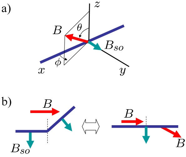
Figure 1: Sketches of the physical systems considered in this work. a) Straight nanowire on the $x$ axis in a homogeneous magnetic field characterized by spherical angles $\theta$ and $\phi$. b) Junction of two nanowires in a uniform magnetic field (left) represented as a straight nanowire with a magnetic inhomogeneity (right).

Summarizing, superconductor, Rashba spin-orbit and Zeeman effects are parametrized in Eq. (1) by $\Delta_{s}$, $\alpha$ and $\Delta_{B}$, respectively. These parameters are taken constant because the nanowire is considered to be made of an homogeneous material. The only inhomogeneity allowed in certain cases is a change in the magnetic field direction at a single magnetic interface between two homogeneous regions.

Along this work the Hamiltonian of Eq. (1) is solved for homogeneous parameters in the infinite, semi-infinite and finite wires, as well as for the inhomogeneous finite case, using different approaches. When a direct diagonalization of the Hamiltonian for a finite system is performed, soft potential edges and magnetic interface are used. The shape of the potential edges is modeled as Fermi-like functions centered on those edges. High potential is imposed outside the nanowire while low potential (usually zero) is assumed inside. When a magnetic interface is present a smooth variation in the field angles is modeled in the same way. Specifically, those smooth functions read

$$V(x) = V_{0}\left[1+{\cal F}(x;x_{L},s_{v})-{\cal F}(x;x_{R},s_{v})\right]\;,$$ (2)

$$\theta(x) = \theta_{L}+(\theta_{R}-\theta_{L})\left[1-{\cal F}(x;x_{m},s_{m})\right]\;,$$ (3)

$$\phi(x) = \phi_{L}+(\phi_{R}-\phi_{L})\left[1-{\cal F}(x;x_{m},s_{m})\right]\;,$$ (4)

for the potential and the field polar and azimuthal angles, respectively. The Fermi function ${\cal F}$ is defined as

$${\cal F}(x;x_{0},s)=\frac{1}{1+e^{(x-x_{0})/s}}\;.$$ (5)

In Eq. (2) $V_{0}$ is the value of the potential outside the nanowire while $\theta_{L/R}$ and $\phi_{L/R}$ are the field angles at left and right of the magnetic interface. The potential left and right edges are centered on $x_{L}$ and $x_{R}$ and the magnetic interface is centered on $x_{m}$. Their softness is controlled by the parameters $s_{v}$ and $s_{m}$, where zero softness means a steep interface and a high value implies a smooth one.

The numerical results of this work are presented in special units obtained by taking $\hbar$, $m$ and the Rashba spin-orbit interaction $\alpha$ as reference values. That is, our length and energy units are

$$L_{\it so} = \frac{\hbar^{2}}{\alpha m}\,,$$ (6)

$$E_{\it so} = \frac{\alpha^{2}m}{\hbar^{2}}\,.$$ (7)

III A sine rule

Let us consider a nanowire in a uniform magnetic field with $\theta=90^{\circ}$ and an arbitrary $\phi$ (see Fig. 1a). A direct diagonalization of Eq. (1) for a finite length of the wire and $\phi=15^{\circ}$ yields the spectrum depicted in Fig. 2 as a function of the magnetic field intensity. A main feature of this figure is the existence of a Majorana mode, lying very near zero energy, but only for a particular range of values of the magnetic field. For the parameters of the figure the Majorana mode is created around $\Delta_{B}=0.3E_{so}$ and destroyed in a rather abrupt way around $\Delta_{B}=E_{so}$.

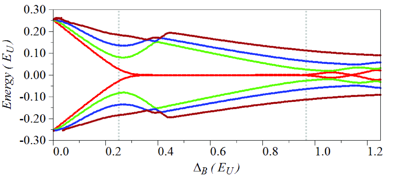
Figure 2: Spectrum of a finite length nanowire with $L=50L_{so}$ as a function of the external magnetic field magnitude $\Delta_{B}$. Other nanowire parameters are $\Delta_{s}=0.25E_{so}$ and $\mu=0$. The magnetic field angles are $\theta=90^{\circ}$ and $\phi=15^{\circ}$. Only the eight states lying closer to zero energy are displayed. Note that a zero energy Majorana mode is created at around $\Delta_{B}=0.3E_{so}$ and destroyed for values of $\Delta_{B}$ near one unit. The vertical lines (dots) indicate the onset and destruction of the Majorana mode as predicted by Eqs. (8) and (13), respectively.

It is well known that Majorana wave functions decay to zero towards the nanowire interior. We can therefore analyze the creation and destruction of Majoranas in the semi-infinite system and use those results to understand the physics of Majoranas in a finite system. In this approach we eliminate from the analysis the finite size effects caused by the overlapping of the Majorana wave functions at both ends of a finite nanowire. Although it is obvious that for long enough wires the size effect becomes negligible, disentangling finite size behavior from intrinsic Majorana physics using calculations of only finite systems is much less obvious.

Majorana mode creation has been understood as a phase transition of the lowest excited state, signaled by the closing and reopening of a gap in the infinite nanowire band spectrum,Oreg et al. (2010) as shown in Figs. 3a and 3b. The phase transition follows in this case a well known law, requiring high-enough fields for Majoranas to exist,

$$\Delta_{B}\geq\sqrt{\Delta_{s}^{2}+\mu^{2}}\;.$$ (8)

Notice that, as mentioned, for the equality in Eq. (8) a gap closes for $k=0$ in Fig. 3b.

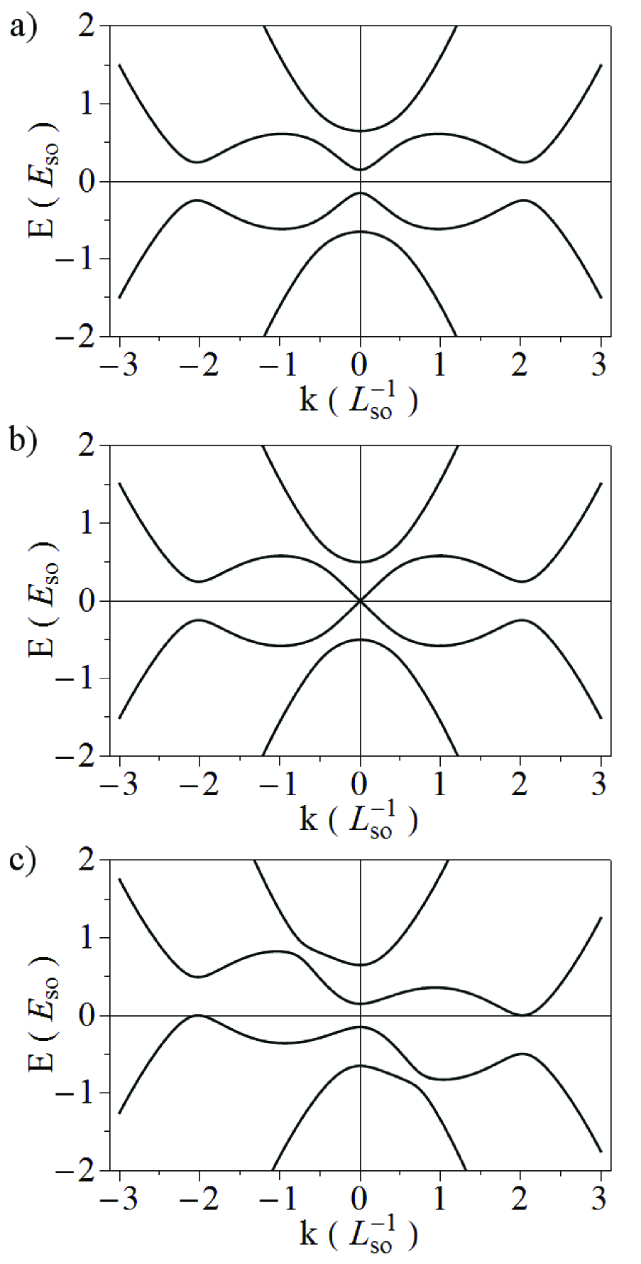
Figure 3: Band structure of the infinite homogeneous nanowire with $\Delta_{s}=0.25E_{so}$ and $\mu=0$ for a) parallel field $(\theta,\phi)=(90^{\circ},0^{\circ})$ with $\Delta_{B}=0.4E_{so}$, b) the same as a) but on the phase transition point $\Delta_{B}=0.25E_{so}$, c) tilted field $(\theta,\phi)=(90^{\circ},38.68^{\circ})$ with $\Delta_{B}=0.4E_{so}$.

In Ref. Serra, 2013 Eq. (8) was derived, in an alternative way, from the analysis of the complex-$k$ solutions compatible with the boundary condition of a semi-infinite nanowire in a parallel field. This approach relies on the property that the complex band structure (allowing an imaginary part in $k$) of the homogeneous wire contains all the information about all possible eigenstates of any piecewise homogeneous wire. In general, an eigenstate of the infinite homogeneous wire with a given arbitrary $k$ can be expressed as

$$\Psi^{(k)}(x,\eta_{\sigma},\eta_{\tau})=\sum_{s_{\sigma},s_{\tau}}\Psi_{s_{\sigma}s_{\tau}}^{(k)}\,e^{ikx}\,\chi_{s_{\sigma}}(\eta_{\sigma})\chi_{s_{\tau}}(\eta_{\tau})\;,$$ (9)

where $\Psi_{s_{\sigma}s_{\tau}}^{(k)}$ are state amplitudes and the quantum numbers are $s_{\sigma}=\pm$ and $s_{\tau}=\pm$.

The sharp semi-infinite wire with $x>0$ is obviously piecewise homogeneous, implying that the Majorana solution allowed by the existence of an edge at $x=0$ must be a linear superposition of the homogeneous nanowire eigenstates of complex wave number with ${\rm Im}(k)>0$, otherwise it could not be a localized state. The resulting restriction is

$$\sum_{k,\,{\rm Im}(k)>0}C_{k}\Psi_{s_{\sigma}s_{\tau}}^{(k)}=0\;,$$ (10)

where the $C_{k}$’s are complex numbers characterizing the superposition of state amplitudes. The allowed wave numbers are calculated solving the determinant

$${\rm det}\left\{H_{s_{\sigma}s_{\tau},s^{\prime}_{\sigma}s^{\prime}_{\tau}}(k)-E\,\openone\right\}=0\;,$$ (11)

for $E=0$. In fact, the allowed $k$’s can be calculated for any energy but we are interested in particular in those at zero energy corresponding to Majorana solutions.

The wave number dependence on magnetic field is depicted in Fig. 4a for a selected case. For a fixed energy $E$ there are always eight possible wave numbers, but only those with ${\rm Im}(k)>0$ are displayed in Fig. 4a. In this representation the closing of the $k=0$ gap in Fig. 3b corresponds to a node of ${\rm Im}(k)$ in Fig. 4a. In order to be able to hold a Majorana a semi-infinite nanowire has to fulfil two simultaneous requirements. First, the nanowire must have four complex wave numbers with ${\rm Im}(k)>0$ allowed at zero energy; and second, a solution different from zero (nontrivial) must be possible for the $C_{k}$’s in Eq. (10). That is, interpreting the state amplitudes $\Psi^{(k)}_{s_{\sigma}s_{\tau}}$ as a $4\times 4$ matrix where the four $k$’s correspond for instance to rows and the four spin-isospin values $\{++,+-,-+,--\}$ to columns, the condition for a nontrivial solution is

$${\rm det}\{\Psi_{s_{\sigma}s_{\tau}}^{(k)}\}=0\;.$$ (12)

In a parallel field this condition is fulfilled only above a critical value of the magnetic field $\Delta^{(c)}_{B}=\sqrt{\Delta^{2}+\mu^{2}}$, but not under this quantity, thus leading to Eq. (8). Further details on the methodology can be found in Ref. Serra, 2013. Here we want to use this approach to determine whether a similar condition on the field orientation, with critical values of the angles, exists or not.

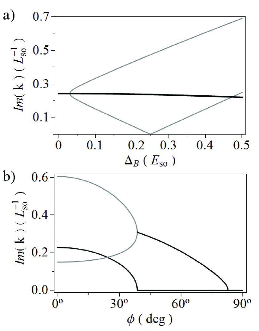
Figure 4: Imaginary parts of the wave numbers (only positive ones) in an infinite homogeneous nanowire with $\Delta_{s}=0.25E_{so}$ and $\mu=0$ as function of a) the value of the longitudinally oriented magnetic field, b) the azimuthal angle $\phi$ of a magnetic field with $\Delta_{B}=0.4E_{so}$ and polar angle $\theta=90^{\circ}$. Gray color is used for non degenerate modes while black is indicating degeneracy with two or more modes actually having the same ${\rm Im}(k)$.

Figure 4b shows the evolution of the wave numbers when increasing $\phi$ while maintaining $\theta=90^{\circ}$, i.e., maintaining the magnetic field in the plane formed by the nanowire direction and the effective spin orbit magnetic field direction $\vec{B}_{so}$. This means that for $\phi=0^{\circ}$ the magnetic field is aligned with the nanowire, while for $\phi=90^{\circ}$ it is completely perpendicular to it and parallel to $\vec{B}_{so}$. In Fig. 4b care has been taken to choose a value of $\Delta_{B}$ that fulfills the Majorana condition for the parallel $\phi=0$ orientation Eq. (8). We can see that for $\phi=40.1^{\circ}$ two of the complex wave numbers become real, thus destroying the Majorana mode for azimuthal angles above this value.

The physical behavior implied by Fig. 4b is a sudden loss of the Majorana mode as the tilting angle $\phi$ exceeds a critical value, due to the system no longer having the required four evanescent modes with ${\rm Im}(k)>0$. The evanescent modes are lost because of the closing of the gap between states of opposite wave numbers ($k\approx\pm 2L_{\it so}^{-1}$ for the particular case shown in Fig. 3c). We characterize next the dependence of the critical angle on $\Delta_{B}$ and $\Delta_{s}$. In Fig. 5a we can see a contour plot of ${\rm Im}(k)$ as a function of $\phi$ and the ratio $\Delta_{s}/\Delta_{B}$ for an external branch wave number,Klinovaja and Loss (2012) corresponding to the lower black line of Fig. 4b. The values where ${\rm Im}(k)$ vanish separate the plot into two regions, the lower one where the Majorana is allowed and the upper (white) where no Majorana can exist. Although Eq. (11) can be solved analytically, the angles where ${\rm Im}\big{(}k(\phi,\Delta_{s}/\Delta_{B})\big{)}$ vanishes can be obtained only numerically because $\phi$ appears as argument of sine and cosine functions and no isolation is possible. As a consequence, the values of $\phi$ where the wave number first reaches zero have been found numerically and are plotted in Fig. 5c against the test function $\arcsin(\Delta_{s}/\Delta_{B})$. The perfect coincidence between the two results within computer precision demonstrates that a Majorana can not exist for angles such that $\sin\phi>\Delta_{s}/\Delta_{B}$, provided $\theta=90^{\circ}$.

Figure 5b shows a contour plot of ${\rm Im}(k)$ for an internal branch wave number,Klinovaja and Loss (2012) corresponding to the upper mode in Fig. 4b. In this plot the $\phi$ roots of ${\rm Im}(k)$ lie inside an upper and lower bounded region around $0.95E_{\rm so}<{\Delta_{B}}<E_{\rm so}$. In fact, two of the wave numbers become real in the white region of the contour plot. Note that this region lies in the non Majorana sector, above the transition discussed in panel a) which is now signaled by the dotted line. Theoretically the existence of this region determines two different fermionic regimes. One where a fermion mode at zero energy is constructed of plane waves with two complex and two real wave numbers and another one made of a full set of real wave numbers. Since we assume bound states in order to extrapolate the results to finite systems, these cases have no relevance to us. Nevertheless the underlying causes for the existence of this region will be relevant in the study of the excited states of the finite nanowire. This will be further developed in Sec. IV.

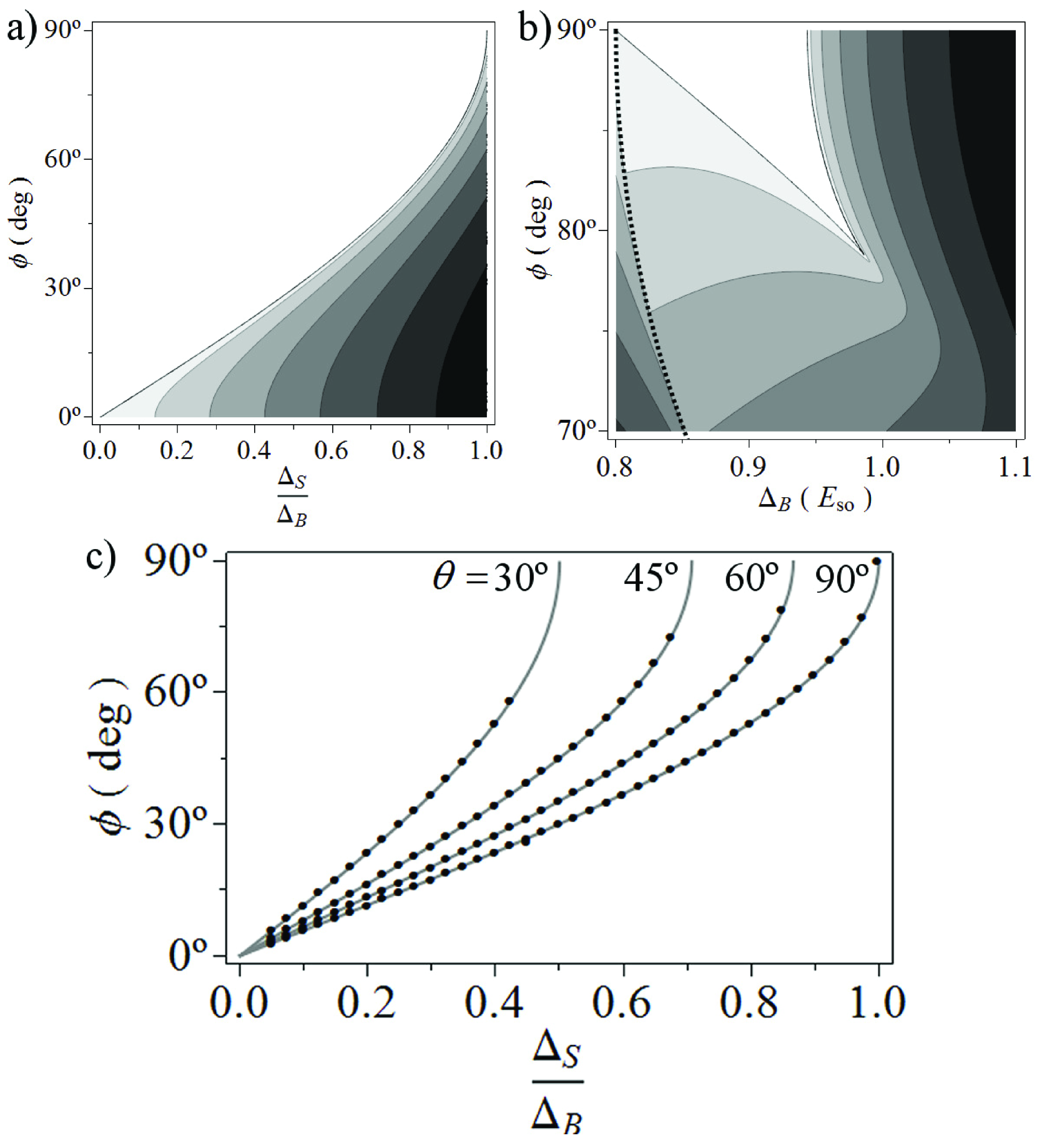
Figure 5: a) Contour plot of ${\rm Im}(k)$ for the external branch of the nanowire propagating bands. The horizontal axis contains the ratio ${\Delta_{s}}/{\Delta_{B}}$ and the vertical one the azimuthal angle $\phi$. The polar angle is fixed to $\theta=90^{\circ}$ and $\mu=0$. b) Contour plot of ${\rm Im}(k)$ for the internal branch of the nanowire propagating bands. The horizontal axis shows $\Delta_{B}$ and the vertical one the azimuthal angle $\phi$. The polar angle is fixed to $\theta=90^{\circ}$, $\Delta_{s}=0.8E_{so}$ and $\mu=0$. c) Plot of the azimuthal critical angle where ${\rm Im}(k)$ vanishes in the upper left panel as function of ${\Delta_{s}}/{\Delta_{B}}$ (points) checked against the sine rule prediction Eq. (13). Besides the $\theta=90^{\circ}$ case of the upper left panel, the figure also contains the comparison for other values of $\theta$. The value of the chemical potential can be taken arbitrarily since it is irrelevant for this comparison.

Repeating the analysis for different polar angles $\theta$, as shown in Fig. 5c, we conclude that the angular restriction for the existence of Majoranas is

$$\Delta_{B}\sin\theta\sin\phi<\Delta_{s}\;.$$ (13)

In other words, the projection of the magnetic field energy parameter into the spin orbit effective magnetic field $\vec{B}_{so}$ needs to be smaller than the superconductor gap energy in order to have Majoranas in a semi-infinite wire. We refer to this condition as the sine rule. Notice that Eq. (13) is not a generalization of Eq. (8), but an additional law. Both Eq. (8) and Eq. (13) have to be simultaneously met for the existence of a Majorana mode in a semi-infinite wire.

In general, the sine rule Eq. (13) yields an extra bound to be considered when identifying regions of Majoranas in parameter space. For instance, assuming fixed angles $(\theta,\phi)$ and varying $\Delta_{B}$ there is a lower bound on $\Delta_{B}$ from Eq. (8) and an upper bound from the sine rule. Analogously, if for a fixed $\Delta_{B}$ the Majorana is allowed by Eq. (8) at $\phi=0^{\circ}$ and and we increase $\phi$ the sine rule yields an upper bound on $\phi$. Therefore, as explained, both equations must be met simultaneously to obtain a Majorana mode. Furthermore, after some parameter testing we have determined that the sine rule is not affected by the value of the chemical potential $\mu$. This means that the overall dependence on $\mu$ for the existence of Majorana modes in the semi-infinite nanowire is completely covered by Eq. (8).

The disappearance of the Majorana when increasing $\phi$ is not a phase transition in the sense that no imaginary part of a mode wave number crosses zero in between two regions with non null values. As shown in Fig. 4b for the polar angle $\theta=90^{\circ}$, above the critical $\phi$ the value of ${\rm Im}(k)$ remains stuck at zero value. The main difference between the phase transition law in Eq. (8) and the sine rule Eq. (13) lies in the different type of gap closing for both cases. As shown in Fig. 3b the phase transition delimited by Eq. (8) is caused by a gap closing and reopening on a single wave number $k=0$ (labeled as interior branches of the spectrum). In the language of semiconductor band structure physics we may call this the closing of a direct gap. Oppositely, the sine rule is caused by the closing of an indirect gap for $k\approx\pm k_{f}$ (labeled as exterior branches of the spectrum), as shown in Fig. 3c for a selected case.

We have checked these laws against the direct numerical diagonalization for a finite nanowire, finding a reasonable agreement as shown in Figs. 2 and 6. In Fig. 2 the magnetic field orientation is kept fixed to a tilted orientation while the field magnitude is changed and in Fig. 6 the magnitude is fixed while the orientation is changed. The main difference between the precise laws for the semi-infinite model and the finite system results is in the smoothness of the spectrum evolution around the transition points. While in the semi-infinite model the transition between fermionic modes to Majorana modes and vice versa happens at a single point in the parameter space, in the finite system we can see these transitions smoothed. This occurs due to the finite size effects, i.e., the little overlap of Majoranas on opposite ends of the nanowire. Furthermore, while Majoranas lie at exactly zero energy in the semi-infinite model, this small interaction makes the finite system Majoranas to have a finite small energy $\epsilon$.

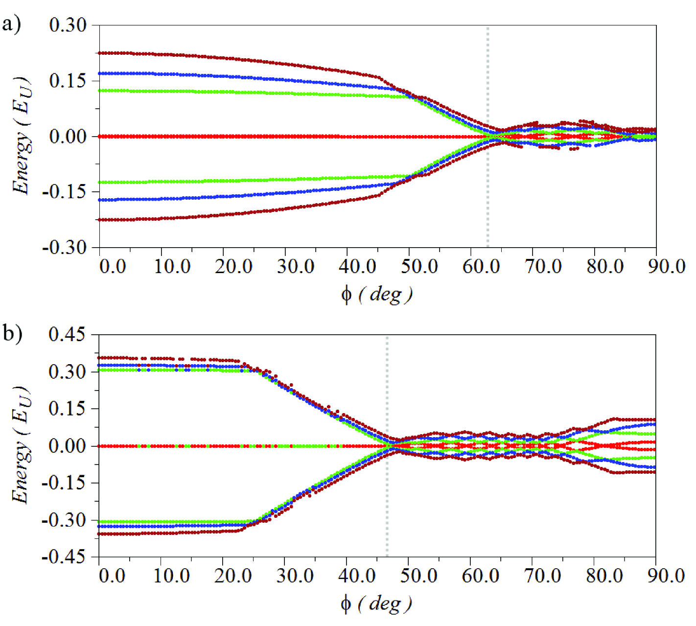
Figure 6: a) Spectrum of a nanowire of length $L=50L_{\rm so}$ with $\Delta_{s}=0.8E_{so}$ and $\mu=0$ as a function of $\phi$ with a fixed $\theta=90^{\circ}$ and $\Delta_{B}=0.9E_{so}$. Note the spectrum change at the angle predicted by the sine rule (dotted line) as well as the spectrum collapse for values of $\phi$ close to $90^{\circ}$. For values of $\phi$ above $90^{\circ}$ the spectrum is given by the mirror image of the shown values. b) The same as a) but for a fixed magnetic field value $\Delta_{B}=1.1E_{so}$. Note that for values of $\phi$ close to $90^{\circ}$ now the two modes closer to zero are fermionic modes separated from each other by an energy gap.

A close inspection of the sine rule Eq. (13) reveals that there exist critical values for $\theta$ and $\phi$ such that if they are not surpassed a Majorana is always allowed, independently of the value of the other angle (provided Eq. (8) is fulfilled). That is, below the critical angle a projection into $\vec{B}_{so}$ is never high enough to break the Majorana. In practice, if the Majorana is allowed by Eq. (8), it will survive for any $\phi$ provided $\theta<\theta_{c}$ or, alternatively, for any $\theta$ provided $\phi<\phi_{c}$. These critical angles are

$$\theta_{c}=\phi_{c}=\arcsin\left(\frac{\Delta_{s}}{\Delta_{B}}\right)\;.$$ (14)

IV Excited states

While in the preceding section we focussed on the physics of the Majoranas at zero energy, comparing semi-infinite and finite nanowires, in this section we address the spectrum of excited states. The main effect of the boundary conditions is to allow only a discrete set of wave numbers instead of a continuous one. What we have done is sketch the finite nanowire spectrum by selecting wave numbers at regular intervals and tracking the evolution of their energy levels with an increasing angle $\phi$. For these examples we maintain the polar angle $\theta=90^{\circ}$ because this is the most physically interesting configuration due to the possibility of aligning external and spin-orbit magnetic fields; nevertheless, analogous plots can be done for different values of $\theta$. The resulting spectrum, shown in Fig. 7, explains the main features of the numerical diagonalization results of Fig. 6 for the same parameters.

In principle, we could also set the boundary conditions exactly as we did in Eq. (10), but we have found this approach impossible to follow on a practical level. The resulting set of equations reads

$$\sum_{k}C^{(L)}_{k}\Psi_{s_{\sigma}s_{\tau}}^{(k)}e^{-i{kL}/{2}}=0\;,$$

$$\sum_{k}C^{(R)}_{k}\Psi_{s_{\sigma}s_{\tau}}^{(k)}e^{i{kL}/{2}}=0\;,$$ (15)

where $C^{(L)}_{k}$ and $C^{(R)}_{k}$ are the coefficients at the left and right nanowire ends, respectively. Basically, the resulting matrix from Eq. (15) is ill defined since it contains very large and very small matrix elements.

The spectra of both panels of Fig. 7 can be divided into three different regions depending on the angle $\phi$. First, for low values of $\phi$ there is a region where a Majorana mode exists and is topologically protected. In Fig. 7 the Majorana is not seen since only excited states of real wave number are shown, but we can see the corresponding gap. For values of $\phi$ above those determined by the sine rule the Majorana mode is destroyed and we can see a region of many level crossings. This behavior of the spectrum is explained by the gap closing of the external branches of the conduction band noticing that in the finite model only some discrete values are allowed, as sketched in Fig. 8. Finally, for higher angular values the region of zero crossings finishes and a third region arises with two possible behaviors.

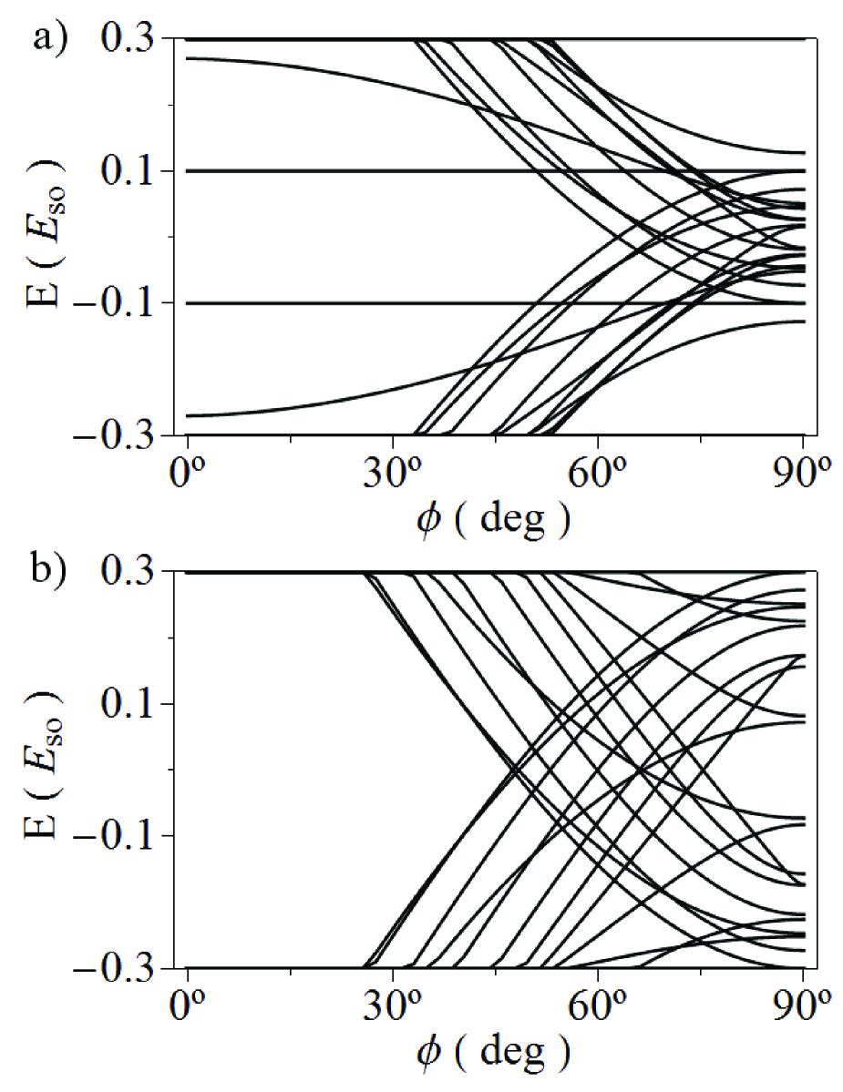
Figure 7: Spectrum obtained from the homogeneous nanowire band energies at selected wave numbers, displayed as tracers as a function of $\phi$. Panel a) corresponds to the same parameters of Fig. 6a. Note that qualitatively similar regions occur for increasing angles in both figures. In particular the spectrum nearly collapses for values of $\phi$ close to $90^{\circ}$. Panel b) shows the same as a) but for the parameters of Fig. 6b. Note that for values of $\phi$ close to $90^{\circ}$ the two lower states (closer to zero energy) are fermionic modes separated by a gap as in Fig. 6b.

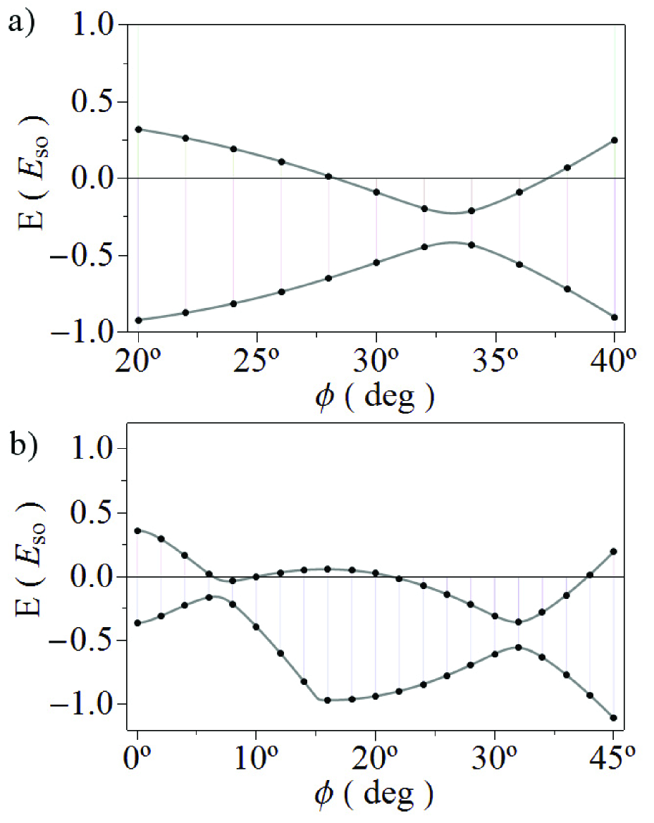
Figure 8: Approximate spectrum of a finite nanowire in a particular configuration of the external magnetic field. a) With only two positive real wave numbers. b) With four positive real wave numbers.

As shown in Figs. 6 and 7 for high $\phi$ angles (near $90^{\circ}$), depending on the parameters the spectrum either opens a gap or collapses near zero energy. The behavior depends on the way the internal branches of the band cross the zero energy value for those angles. The internal branches of the band can cross the zero energy level for high angles in one $k>0$ point, like in Fig. 8a, thus leading (jointly with the external branch crossing point) to four real and four complex wave numbers; or, alternatively, the interior brach can cross zero energy in more than one $k>0$ point, like in Fig. 8b, leading to wavefunctions characterized by eight real wave numbers. In the latter case there is a wave number range where the band spectrum lies very close to zero energy, yielding this way a collapse of the finite wire spectrum. The particular set of parameters where one or the other situation happens depends on the behavior of the internal branches of the band structure and it is not as easily predictable as the behavior of the external branches that led to the sine rule. The region of values where this collapse arises coincides with the region where the allowed solutions at zero energy are made of real wave numbers only and it was already presented in Fig. 5a for the $\mu=0$ case.

V Magnetic inhomogeneity models

In this section we explore the physics of a junction of two straight nanowires with a certain angle in presence of a homogeneous magnetic field parallel to one of the arms, as sketched in Fig. 1b. We assume a representation of the system as a single straight 1D nanowire containing a magnetic interface. The inhomogeneity separates two homogeneous regions with different directions (but the same magnitude) of the external magnetic field. The system is solved by numerical diagonalization, assuming a soft magnetic interface, interpreting the results by comparing with the homogeneous nanowire discussed in the preceding section. We focus on two specific effects, tilting and stretching of one of the two junction arms.

V.1 Arm tilting

The magnetic field is aligned with the left arm and the spectrum of the nanowire is computed for varying orientations of the field in the the right arm (see Fig. 9). As mentioned, this model represents under certain approximations a bent nanowire in a homogeneous magnetic field. It was shown in Ref. Wu et al., 1992 that bent nanowires can be approximated by 1D models with a potential well simulating the effect of the bending. Here we have only considered the magnetic field change of direction as the main inhomogeneity source, disregarding the electrical potential effects of the bending.

The spectrum of the inhomogeneous nanowire can be explained in terms of the homogeneous one for a tilted magnetic field. Figure 9 compares the inhomogeneous (upper) with the homogeneous (lower) nanowire spectrum for the same set of parameters, showing that both results share the same essential features. More precisely, three $\phi$ regions can be found in both cases, but with two main differences. First, while for the homogeneous nanowire increasing $\phi$ leads to the destruction of the Majoranas on both ends, for the inhomogeneous nanowire only the right side Majorana is destroyed. The density of the Majorana for the inhomogeneous nanowire is shown in Figs. 10 and 11 for selected values of the parameters. As a consequence, the bent junction holds a Majorana mode (the one localized in the left side of the inhomogeneity) independently of the magnetic angle at the right side.

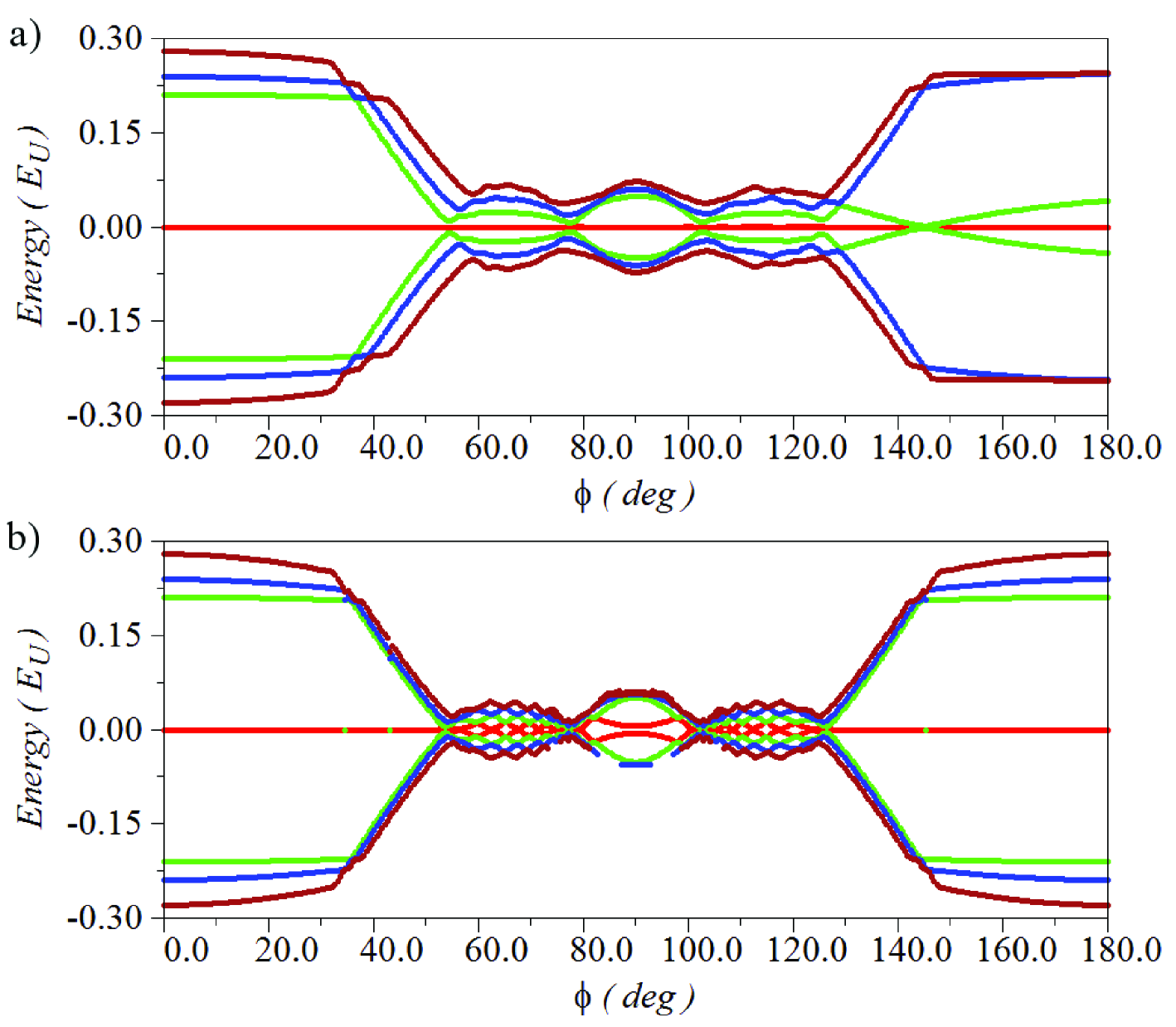
Figure 9: a) Nanowire spectrum for $\Delta_{s}=0.8E_{so}$ and $\mu=0$ with a magnetic inhomogeneity at its center as a function of the tilting angle $\phi$. On the left side of the nanowire the magnetic field is parallel, while on the right side its angles are $(\theta=90^{\circ},\phi)$. The magnetic field strength is constant in both sides and equal to $\Delta_{B}=E_{so}$. b) Spectrum of a nanowire in a homogeneous magnetic field with angles $(\theta=90^{\circ},\phi)$ and with the rest of parameters as in a).

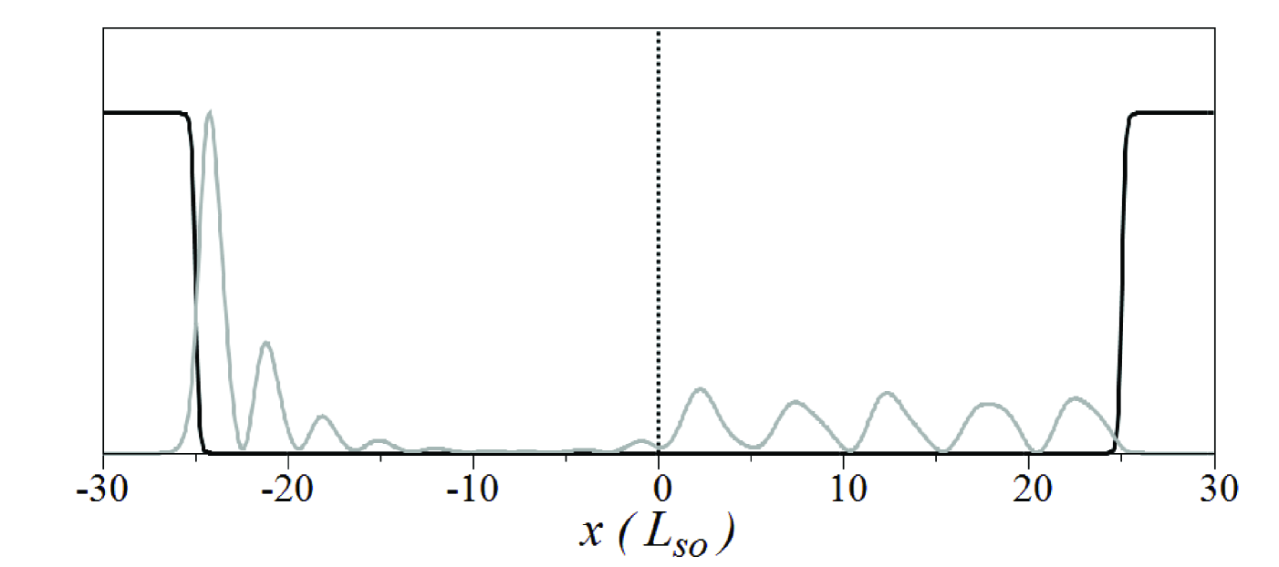
Figure 10: Majorana density function of an inhomogeneous nanowire similar to the one described in Fig. 9a. The magnetic field azimuthal angles in the two arms are $\phi_{L}=0^{\circ}$ and $\phi_{R}=90^{\circ}$, while all along the nanowire it is $\theta=90^{\circ}$. Other parameters are $\Delta_{B}=0.4$, $\Delta_{s}=0.25$.

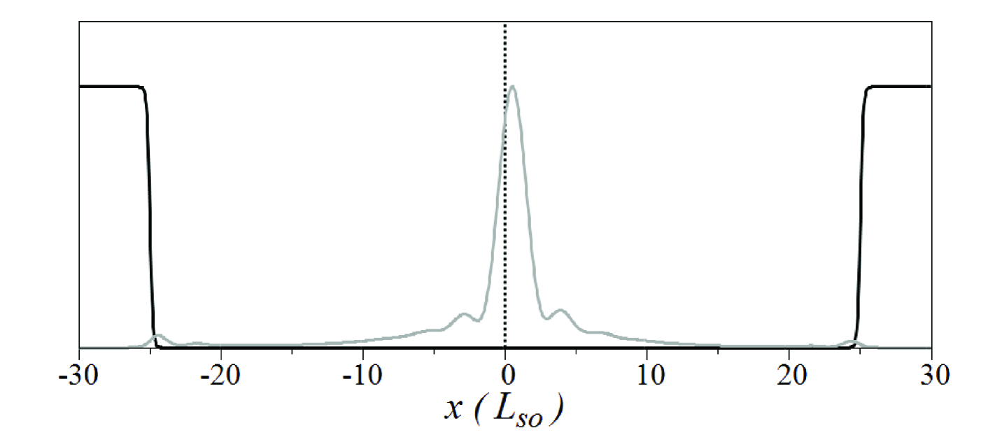
Figure 11: Density function of the first excited state of the inhomogeneous nanowire of Fig. 9a. This state becomes localized at the magnetic inhomogeneity for an azimuthal angle $\phi=145^{\circ}$ (and polar angle $\theta=90^{\circ}$).

A second difference between upper and lower panels of Fig. 9 is that the spectra for the inhomogeneous nanowire is not symmetric with respect to $\phi=90^{\circ}$, in contrast with the homogeneous nanowire. A zero energy crossing localized in the inhomogeneity interface arises at $\phi=145^{\circ}$ for the selected parameters in Figs. 9a and 11. The corresponding bound state originates in the second excited state of the system and it is not Majorana in nature. Furthermore, this localized state is caused completely by the magnetic inhomogeneity and has no relationship with the localized states found in the bending region in Ref. Wu et al., 1992 because we have disregarded those effects. Although we know these states are related with the magnetic inhomogeneity, a deep understanding of their causes and the particular set of parameters leading to their enhancement or quenching is yet to be understood.

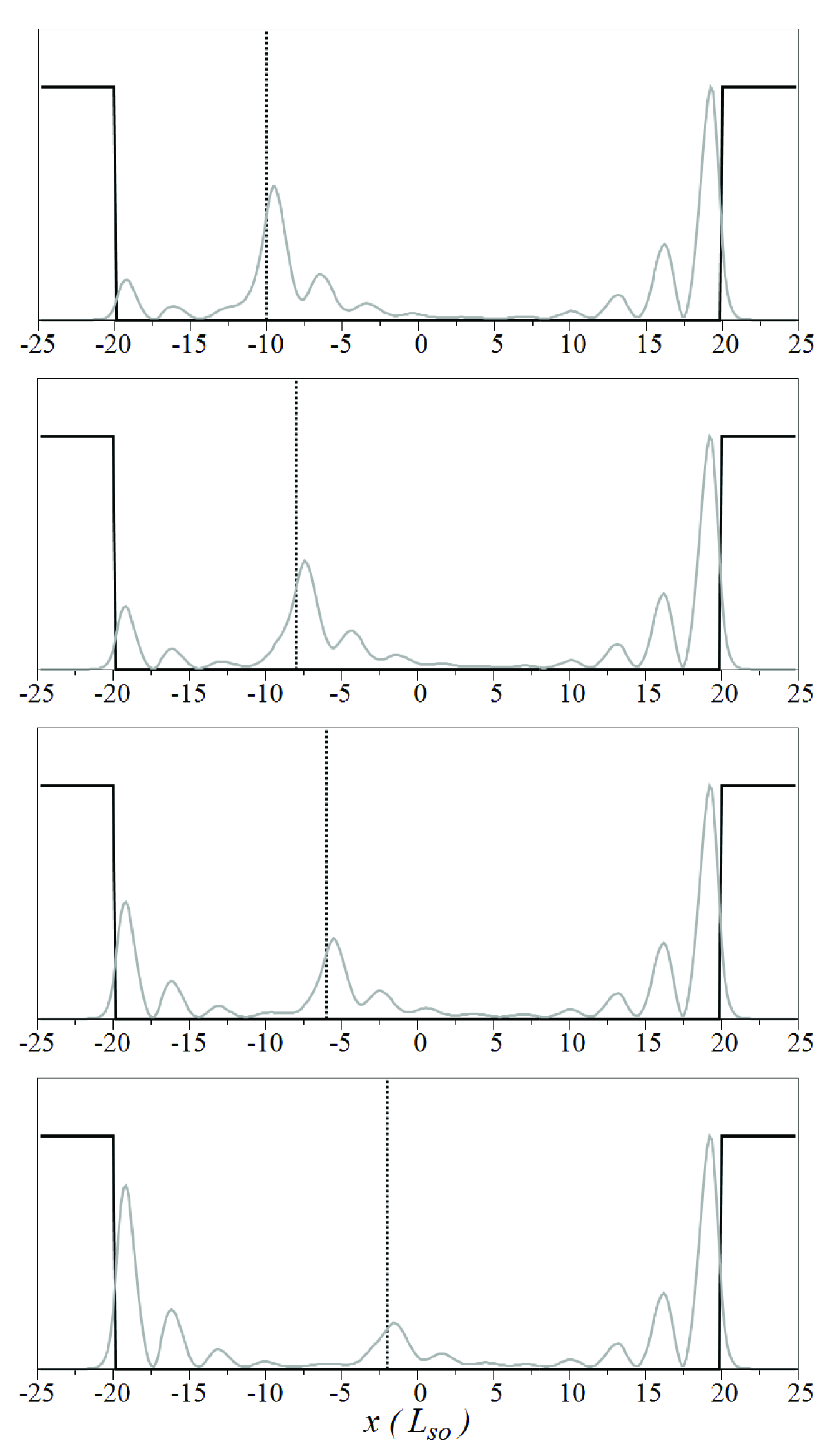
Figure 12: Density distributions of the Majorana mode in a finite nanowire with a magnetic inhomogeneity. We used $\Delta_{s}=0.25E_{so}$, $\mu=0$ and a magnetic field of magnitude $\Delta_{B}=0.4E_{so}$ oriented parallel in the left side of the magnetic interface and antiparallel in the right side. In each panel the potential well and the position of the magnetic interface are shown. The latter corresponds to a Fermy-type function whose position shifts to the right following the sequence from upper to lower panels.

V.2 Arm stretching

We study now the behavior of the Majorana modes in the nanowire as a function of the inhomogeneity distance to the nanowire end. The magnetic field directions are fixed at $(\theta=90^{\circ},\phi=0^{\circ})$ on the left end and $(\theta=90^{\circ},\phi=180^{\circ})$ on the right end of the nanowire. This is a particularly interesting configuration as it is the only setup where both ends lie inside a longitudinal magnetic field, apart from the homogeneous case. This way, all the observed effects must be caused by the inhomogeneity and its distance with respect to the left nanowire end.

Figure 12 shows the probability densities of the zero energy state at different positions of the magnetic interface with respect the left side of the nanowire. From upper to lower panels of Fig. 12 we may follow the evolution as the distance of the magnetic interface to the left end of the system is increased. Most remarkably, for short distance the left Majorana is not peaked on the left end, but remains stuck on the magnetic interface (upper panels). If the distance is increased, however, the Majorana is eventually transferred to the left nanowire end after some critical distance (lower panels). This transfer is seen as a smooth decrease of the density maximum at the magnetic interface accompanied by an increase at the left end. Finally, when the interface is on the middle point of the nanowire both Majoranas are located at their corresponding ends. It is also worth noticing that this Majorana transfer does not imply a departure of the mode from zero energy because the Majorana on the other end of the nanowire is not affected (see Fig. 13). Additionally, the transfer phenomenon is not caused by finite size effects since we have checked that it happens for the same characteristic distance when the right end is further displaced to the right.

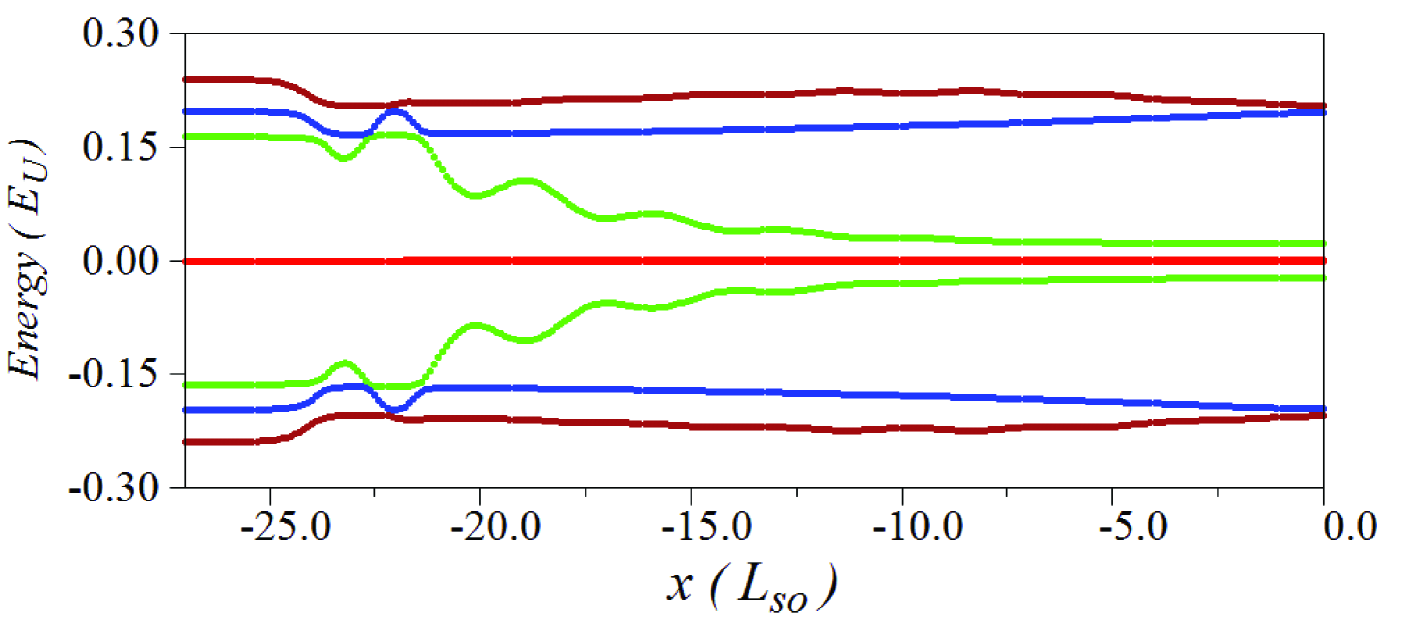
Figure 13: Spectrum of the nanowire described in the caption of Fig. 12 as a function the magnetic interface position.

VI Conclusions

In this work we have studied the spectra of 1D nanowires for arbitrary orientation of the magnetic field, focussing in particular on the conditions leading to a Majorana mode. This study has been realized from different perspectives and methods in an effort to explain the variety of observed phenomena. We have combined the complex band structure techniques of infinite homogeneous nanowires with numerical diagonalizations of finite systems.

We have demonstrated an additional condition, besides the well known topological transition law, that needs to be taken into account in order to predict the regimes of existence of Majorana modes with tilted fields. We have named this additional condition the sine rule. The sine rule predicts an upper bound on the magnetic field at which Majoranas are to be found in a 1D wire with tilted field. When the topological law is fulfilled, the sine rule leads to critical values of the field angles $\theta_{c}$ and $\phi_{c}$, such that a Majorana mode is always found for any $\phi$ provided $\theta<\theta_{c}$ or, alternatively, for any $\theta$ provided $\phi<\phi_{c}$.

We have extended our analysis to nanowire junctions with an arbitrary angle, modeled as magnetically inhomogeneous nanowires, explaining most of their properties in terms of the behavior of its homogeneous parts. We have focussed, particularly, on the role of tilting and stretching of one of the junction arms. We also reported the existence of a bound non Majorana state located on the magnetic inhomogeneity. Finally, we have studied the Majorana transfer phenomenon as the distance of the magnetic inhomogeneity to the nanowire end is increased. Testing these predictions would require experiments of nanowires in inhomogeneous magnetic fields. Alternatively, it has been suggested in this work that a bent nanowire in a homogeneous field should display similar phenomena, while being more feasible in practice. As an interesting continuation of this work we are presently analyzing the validity of the sine rule in higher dimensional nanowires, where the transverse degrees of freedom require a multimode description of the electronic states.