Migration paths saturations in meta-epidemic systems.

Abstract

In this paper we consider a simple two-patch model in which a population affected by a disease can freely move. We assume that the capacity of the interconnected paths is limited, and thereby influencing the migration rates. Possible habitat disruptions due to human activities or natural events are accounted for. The demographic assumptions prevent the ecosystem to be wiped out, and the disease remains endemic in both populated patches at a stable equilibrium, but possibly also with an oscillatory behavior in the case of unidirectional migrations. Interestingly, if infected cannot migrate, it is possible that one patch becomes disease-free. This fact could be exploited to keep disease-free at least part of the population.

1 Introduction

Natural landscapes can become fragmented due to landslides, for instance, or human constructions. Wild populations can be affected by these events. To understand these phenomena and possibly alleviate their negative consequences for the environment, scientists have developed the concepts of population assembling, [10], and metapopulations, [8, 19], which showed that global survival is possible even if in some patches the populations get extinguished, [18].

Diseases represent a common occurrence in nature for individuals and communities. Ecoepidemiology merges the demographic and epidemiological features of interacting populations into a single model, see Chapter 7 of [11] for an introduction. In this context also metaecoepidemic models can be considered, [13].

Epidemics affecting populations living in patchy habitats have been investigated since quite some time, also in the context of fighting new emerging diseases, both deterministically, [3, 12, 14, 16, 17], and stochastically, [4].

We consider a very simple one disease-affected population, 2-patch model with migrations. In [5, 6] other models of this kind have been introduced. A specific feature of this contribution lies in the fact that an upper bound on the migration rates is assumed, as in [1], but the restrictive assumption of no vital dynamics used for that similar model is here removed. Of interest is the assessment of the consequences that possible paths disturbances have on the whole ecosystem. The disease is assumed to be recoverable, but both disease transmission and recovery rates are environment-dependent. The disease tranmission is modeled via mass action, assuming homogeneous mixing for the population in both patches. Instead in [2] $n$ patches are assumed, where SIS models with standard incidence are present in each one. No vital dynamics is however considered. In [7] the model is similar to [2], but contains susceptible recruitments and a different disease incidence.

The effect of population diffusion on the disease spread is studied in [15], investigating what happens if the disease gets eradicated in neighboring patches. Also, diffusion may or may not help the epidemics to spread, [16].

The main reference model is [9], where the environment consists of several fragments. The stability conditions for endemic and disease-free equilibria are established. In contrast to [9], we propose here a saturation effect on the migrating corridors. The analysis of course shows that the basic equilibria are the same, i.e. system disappearance and the endemic equilibrium with both patches populated. Further, we also try to answer the question of what happens to the ecosystem as a whole when some disruptions in the interpatch communications occur. This could happen because migrations are not possible in one direction, or if they require a strenuous effort, which infected individuals cannot exert.

2 The Model

A similar model with restricted migrations has been introduced in [1]. But in contrast to its assumptions stating that the migrations are restricted by the size of the population of the patch into which the migration occurs, we rather consider here the case in which migrations are restricted by the size of the available canals. Thus, even if the populations in each patch grow, only a maximal fixed migration rate can be attained. Mathematically, this is obtained by using a Holling type II function for modelling the migration rates.

For $k=1,2$, let us denote by $S_{k}$ the susceptibles and by $I_{k}$ the infected in each patch.

$$\dot{S_{1}}=r_{1}S_{1}-\gamma_{1}S_{1}I_{1}+\delta_{1}I_{1}-m_{21}\frac{S_{1}}{A+I_{1}+S_{1}}+m_{12}\frac{S_{2}}{A+I_{2}+S_{2}},$$ (1)

$$\dot{I_{1}}=\gamma_{1}S_{1}I_{1}-(\delta_{1}+\mu_{1})I_{1}-n_{21}\frac{I_{1}}{B+I_{1}+S_{1}}+n_{12}\frac{I_{2}}{B+I_{2}+S_{2}},$$

$$\dot{S_{2}}=r_{2}S_{2}-\gamma_{2}S_{2}I_{2}+\delta_{2}I_{2}+m_{21}\frac{S_{1}}{A+I_{1}+S_{1}}-m_{12}\frac{S_{2}}{A+I_{2}+S_{2}},$$

$$\dot{I_{2}}=\gamma_{2}S_{2}I_{2}-(\delta_{2}+\mu_{2})I_{2}+n_{21}\frac{I_{1}}{B+I_{1}+S_{1}}-n_{12}\frac{I_{2}}{B+I_{2}+S_{2}}.$$

The parameters have the following meanings. By $r_{k}$ we denote the net reproduction rate of the susceptibles in patch $k$. Note that we make the strong demographic assumption that only susceptibles give birth, the disease preventing the infected to reproduce. Further, $\gamma_{k}$ denotes the disease contact rate, $\delta_{k}$ is the disease recovery rate, $\mu_{k}$ is the infected mortality rate in each patch, $A$ is the half saturation constant for the susceptibles, and $B$ the one for the infected; finally the migration rates from patch $j$ into patch $i$ are $m_{ij}$ for the susceptibles and $n_{ij}$ for the infected. In fact, e.g. the parameter $m_{12}$ represents the maximum migration rate possible for the susceptibles through the canal leading from patch 2 into patch 1. The last term in the first equation states thus that the higher the population in patch 2, the smaller the migration rate becomes in view of the saturation of the communication path. Similarly for the corresponding terms in this and the other equations.

The first equation states that the susceptibles reproduce, and possibly become infected by contagion, new recruits come into this class also via disease recovery, and then the emigrations and immigrations occur. Similar considerations hold true for the remaining equations.

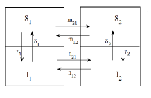
Figure 1: The system in consideration.

2.1 Equilibria

The general model admits only two possible equilibria, the trivial state in which the ecosystem vanishes, and the coexistence state.

To study the latter, we can eliminate the migration rates by summing the first and third equations of (1), as well as the second and fourth one, to obtain respectively

$$r_{1}\tilde{S_{1}}-\gamma_{1}\tilde{S_{1}}\tilde{I_{1}}+\delta_{1}\tilde{I_{1}}+r_{2}\tilde{S_{2}}-\gamma_{2}\tilde{S_{2}}\tilde{I_{2}}+\delta_{2}\tilde{I_{2}}=0,$$

$$\gamma_{1}\tilde{S_{1}}\tilde{I_{1}}-(\delta_{1}+\mu_{1})\tilde{I_{1}}+\gamma_{2}\tilde{S_{2}}\tilde{I_{2}}-(\delta_{2}+\mu_{2})\tilde{I_{2}}=0.$$ (2)

These equations can also be summed, to produce

$$\tilde{S_{1}}=\frac{-r_{2}\tilde{S_{2}}+\mu_{1}\tilde{I_{1}}+\mu_{2}\tilde{I_{2}}}{r_{1}}$$ (3)

which upon substitution into (2) gives

$$\tilde{S_{2}}=\frac{r_{1}((\delta_{1}+\mu_{1})\tilde{I_{1}}+(\delta_{2}+\mu_{2})\tilde{I_{2}})-\gamma_{1}\mu_{1}{\tilde{I_{1}}}^{2}-\gamma_{1}\mu_{1}\tilde{I_{1}}\tilde{I_{2}}}{r_{1}\gamma_{2}\tilde{I_{2}}-r_{2}\gamma_{1}\tilde{I_{1}}}.$$ (4)

We need nonnegative populations, therefore some necessary conditions for the feasibility of the equilibrium with endemic disease and both patches populated follow:

$$\tilde{I_{1}}>\frac{r_{1}\gamma_{2}\tilde{I_{2}}}{r_{2}\gamma_{1}},\quad\tilde{S_{2}}\leq\frac{\mu_{1}\tilde{I_{1}}+\mu_{2}\tilde{I_{2}}}{r_{2}},\quad\tilde{I_{2}}\geq\frac{\gamma_{1}\mu_{1}{\tilde{I_{1}}}^{2}-r_{1}(\delta_{1}+\mu_{1})\tilde{I_{1}}}{r_{1}(\delta_{2}+\mu_{2})-\gamma_{1}\mu_{2}\tilde{I_{1}}}$$ (5)

or the opposite inequalities. The last one, however, leads to an upper bound that must be explicitly imposed not to be negative. In conclusion, we have the second set of necessary conditions

$$\tilde{I_{1}}<\frac{r_{1}\gamma_{2}\tilde{I_{2}}}{r_{2}\gamma_{1}},\quad\tilde{S_{2}}\leq\frac{\mu_{1}\tilde{I_{1}}+\mu_{2}\tilde{I_{2}}}{r_{2}},\quad\tilde{I_{2}}\leq\frac{\gamma_{1}\mu_{1}{\tilde{I_{1}}}^{2}-r_{1}(\delta_{1}+\mu_{1})\tilde{I_{1}}}{r_{1}(\delta_{2}+\mu_{2})-\gamma_{1}\mu_{2}\tilde{I_{1}}},$$ (6)

supplemented by either one of the two sets of conditions,

$$\frac{\delta_{2}+\mu_{2}}{\gamma_{1}\mu_{2}}<I_{1}\leq\frac{\delta_{1}+\mu_{1}}{\gamma_{2}\mu_{1}},\quad\frac{\delta_{1}+\mu_{1}}{\gamma_{2}\mu_{1}}\leq I_{1}<\frac{\delta_{2}+\mu_{2}}{\gamma_{1}\mu_{2}}$$

2.2 Stability

The Jacobian of (1) is

$$J=\left[\begin{array}[]{cccc}J_{11}&-\gamma_{1}S_{1}+\delta_{1}+\hat{\eta_{2}}S_{1}&\hat{\theta_{1}}-\hat{\theta_{2}}S_{2}&-\hat{\theta_{2}}S_{2}\\ \\ \gamma_{1}I_{1}+\hat{\rho_{2}}I_{1}&J_{22}&-\hat{\sigma_{2}}I_{2}&\hat{\sigma_{1}}-\hat{\sigma_{2}}I_{2}\\ \\ \hat{\eta_{1}}-\hat{\eta_{2}}S_{1}&-\hat{\eta_{2}}S_{1}&J_{33}&-\gamma_{2}S_{2}+\delta_{2}+\hat{\theta_{2}}S_{2}\\ \\ -\hat{\rho_{2}}I_{1}&\hat{\rho_{1}}-\hat{\rho_{2}}I_{1}&\gamma_{2}I_{2}+\hat{\sigma_{2}}I_{2}&J_{44}\end{array}\vspace{3pt}\right]$$ (7)

with

$$J_{11}=-\gamma_{1}I_{1}-\hat{\eta_{1}}+\hat{\eta_{2}}S_{1}+r_{1},\quad J_{22}=\gamma_{1}S_{1}-\delta_{1}-\hat{\rho_{1}}+\hat{\rho_{2}}I_{1}-\mu_{1}$$

$$J_{33}=-\gamma_{2}I_{2}-\hat{\theta_{1}}+\hat{\theta_{2}}S_{2}+r_{2},\quad J_{44}=\gamma_{2}S_{2}-\delta_{2}-\hat{\sigma_{1}}+\hat{\sigma_{2}}I_{2}-\mu_{2},$$

$$\hat{\eta_{1}}=\frac{m_{21}}{A+S_{1}+I_{1}},\quad\hat{\eta_{2}}=\frac{m_{21}}{{(A+S_{1}+I_{1})}^{2}},\quad\hat{\theta_{1}}=\frac{m_{12}}{A+S_{2}+I_{2}},$$

$$\hat{\theta_{2}}=\frac{m_{12}}{{(A+S_{2}+I_{2})}^{2}},\quad\hat{\rho_{1}}=\frac{n_{21}}{B+S_{1}+I_{1}},\quad\hat{\rho_{2}}=\frac{n_{21}}{{(B+S_{1}+I_{1})}^{2}}$$

$$\hat{\sigma_{1}}=\frac{n_{12}}{B+S_{2}+I_{2}},\quad\hat{\sigma_{2}}=\frac{n_{12}}{{(B+S_{2}+I_{2})}^{2}}.$$

The origin represents the only case in which the stability study can be performed analytically. The characteristic equation factorizes, to give $H(\lambda)K(\lambda)=0$, with

$$K(\lambda)=\lambda^{2}+(\delta_{1}+\delta_{2}+\mu_{1}+\mu_{2}+\frac{n_{12}}{B}+\frac{n_{21}}{B})\lambda+(\delta_{2}+\mu_{2})(\delta_{1}+\mu_{1}+\frac{n_{21}}{B})+(\delta_{1}+\mu_{1})\frac{n_{12}}{B}$$

and

$$H(\lambda)=\lambda^{2}+(\frac{m_{12}}{A}+\frac{m_{21}}{A}-r_{1}-r_{2})\lambda-\frac{m_{12}r_{1}}{A}-\frac{m_{21}r_{2}}{A}+r_{1}r_{2}.$$ (8)

For $K(\lambda)$ all coefficients are positive, so that its roots have both negative real parts. If we consider the Routh-Hurwitz conditions for $H(\lambda)=0$, we find

$$\frac{m_{12}}{A}+\frac{m_{21}}{A}-r_{1}-r_{2}>0\quad-\frac{m_{12}r_{1}}{A}-\frac{m_{21}r_{2}}{A}+r_{1}r_{2}>0.$$

The stability conditions are then

$$A(r_{2}+r_{1})-m_{21}<m_{12}<Ar_{2}-\frac{m_{21}r_{2}}{r_{1}}.$$

Eliminating $Ar_{2}$ from the first and last terms, and observing that $m_{12}>0$ in the last inequality, we get

$$Ar_{1}-m_{21}<-\frac{m_{21}r_{2}}{r_{1}}\quad A-\frac{m_{21}}{r_{1}}>0,$$

from which $-m_{21}r_{2}r_{1}^{-1}>0$ follows, thus showing that the origin can never be stable.

Through numerical simuations, it can be verified that indeed the endemic equilibrium can be stably achieved. This can be accomplished for instance using the following set of parameter values

$$r_{1}=1,\quad r_{2}=1,\quad\gamma_{1}=1,\quad\gamma_{2}=1,\quad\delta_{1}=0.5,\quad\delta_{2}=0.5,\quad\mu_{1}=1,$$

$$\mu_{2}=1,\quad m_{12}=1,\quad m_{21}=1,\quad n_{12}=1,\quad n_{21}=1,\quad A=1,\quad B=10.$$

2.3 Bifurcations

We now show that no Hopf bifurcations can arise at the origin. Since $K(\lambda)$ has roots with negative real parts, we consider only $H(\lambda)=0$. To have a Hopf bifurcation we need

$$\frac{m_{12}}{A}+\frac{m_{21}}{A}-r_{1}-r_{2}=0,\quad-\frac{m_{12}r_{1}}{A}-\frac{m_{21}r_{2}}{A}+r_{1}r_{2}>0.$$

Solving for $r_{2}$ in the first equation, and substituting into the second one, we have

$$\Psi(r_{1})=-{r_{1}}^{2}+2\frac{m_{21}r_{1}}{A}-\frac{m_{21}}{A}\left(\frac{m_{12}}{A}+\frac{m_{21}}{A}\right)>0.$$

But this condition can never be satisfied, as the concave parabola $\Psi(r_{1})=0$ has the vertex $\left(m_{21}A^{-1},-m_{21}m_{12}A^{-2}\right)$, lying in the fourth quadrant.

3 Unidirectional Migrations

We now consider the case in which the joining path between the two patches can be traversed only in one direction. This is by no means restrictive as for instance fish can swim much more easily downstream in rivers, and sometimes dams and waterfalls prevent them from returning upstream. The Figure 2 describes the situation.

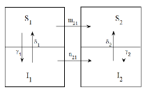
Figure 2: The schematic model of unidirectional migrations.

The system (1) contains now $m_{12}=0$ and $n_{12}=0$. The system’s Jacobian (7) simplifies accordingly.

3.1 Equilibria

In this case we have again the origin, and possibly coexistence. But in addition, we find the point $E_{1}=(0,0,\tilde{S_{2}},\tilde{I_{2}})$ with

$$\tilde{S_{2}}=\frac{\delta_{2}+\mu_{2}}{\gamma_{2}},\quad\tilde{I_{2}}=\frac{r_{2}(\delta_{2}+\mu_{2})}{\gamma_{2}\mu_{2}},$$ (9)

which is always feasible.

We also find the point $E_{2}=(\tilde{S_{1}},0,\tilde{S_{2}},\tilde{I_{2}})$ with population values

$$\tilde{S_{1}}=\frac{m_{21}-r_{1}A}{r_{1}},\quad\tilde{S_{2}}=\frac{\delta_{2}+\mu_{2}}{\gamma_{2}},\quad\tilde{I_{2}}=\frac{\gamma_{2}(m_{21}-r_{1}A)+r_{2}(\delta_{2}+\mu_{2})}{\gamma_{2}\mu_{2}}.$$ (10)

It has the following feasibility condition,

$$m_{21}\geq r_{1}A.$$ (11)

3.2 Stability

At the origin, we find the following eigenvalues,

$$\lambda_{1}=r_{2}\quad,\lambda_{2}=-\delta_{2}-\mu_{2},\quad\lambda_{3}=\frac{r_{1}A-m_{21}}{A},\quad\lambda_{4}=-\frac{\delta_{1}B+n_{21}+\mu_{1}B}{B},$$

from which its unconditional instability is immediate. Since all the eigenvalues are real, no Hopf bifurcation can arise.

At $E_{1}$ again it is possible to obtain directly the eigenvalues,

$$\lambda_{1,2}=\frac{-r_{2}\delta_{2}\pm\sqrt{{r_{2}}^{2}{\delta_{2}}^{2}-4{\mu_{2}}^{2}r_{2}(\mu_{2}+\delta_{2})}}{2\mu_{2}},\quad\lambda_{3}=\frac{-m_{21}+r_{1}A}{A}$$

and $\lambda_{4}=-[(\delta_{1}+\mu_{1})B+n_{21}]B^{-1}<0$. Since also $\lambda_{1,2}<0$ easily, stability is regulated by the third eigenvalue, giving

$$r_{1}A<m_{21}.$$ (12)

Again, no Hopf bifurcations arise, since the eigenvalues $\lambda_{1}$ and $\lambda_{2}$ can never be purely imaginary, as the parameters are all positive: $r_{2}\delta_{2}\neq 0$, since $r_{2}>0$ and $\delta_{2}>0$.

At $E_{2}$ once more the eigenvalues are explicitly found,

$$\lambda_{1}=\gamma_{1}\tilde{S_{1}}-\delta_{1}-\mu_{1}-\frac{n_{21}}{B+\tilde{S_{1}}},\quad\lambda_{2}=-\frac{m_{21}}{A+\tilde{S_{1}}}+\frac{m_{21}\tilde{S_{1}}}{{(A+\tilde{S_{1}})}^{2}}+r_{1},$$

$$\lambda_{3,4}=\frac{r_{2}-\gamma_{2}\tilde{I_{2}}\pm\sqrt{(r_{2}-\gamma_{2}\tilde{I_{2}})^{2}-4\mu_{2}\gamma_{2}\tilde{I_{2}}}}{2}.$$

Using the expression for $\tilde{S_{1}}$ the second eigenvalue becomes $\lambda_{2}=r_{1}(m_{21}-r_{1}A)m_{21}^{-1}$, so that its negativity in this case entails $m_{21}-r_{1}A<0$, which contradicts the feasibility condition (11). In conclusion, $E_{2}$ is unconditionally unstable. Also here no Hopf bifurcations arise. Imposing the real part of $\lambda_{3,4}$ to be zero, we find $r_{2}-\gamma_{2}\tilde{I_{2}}=0$ which explicitly becomes

$$-\frac{\gamma_{2}(m_{21}-r_{1}A)+r_{2}\delta_{2}}{\mu_{2}}=0,$$

which cannot be satisfied in view of the feasibility condition (11).

In this model we can study the coexistence equilibrium, because the Jacobian becomes a lower triangular matrix. The characteristic equation then factorizes accordingly, to give the quadratic equation

$${\lambda}^{2}+a_{1}\lambda+a_{0}=0$$ (13)

with

$$\begin{array}[]{l}a_{1}=\gamma_{1}\tilde{I_{1}}+\tilde{\eta_{1}}-\tilde{\eta_{2}}\tilde{S_{1}}-r_{1}-\gamma_{1}\tilde{S_{1}}+\delta_{1}+\mu_{1}+\tilde{\rho_{1}}-\tilde{\rho_{2}}\tilde{I_{1}}\\ a_{0}=(-\gamma_{1}\tilde{I_{1}}-\tilde{\eta_{1}}+r_{1})(-\delta_{1}-\mu_{1}-\tilde{\rho_{1}}+\tilde{\rho_{2}}\tilde{I_{1}})+\gamma_{1}\tilde{S_{1}}\tilde{I_{1}}(\tilde{\rho_{2}}-\tilde{\eta_{2}})\\ +\tilde{\eta_{2}}\tilde{S_{1}}(\gamma_{1}\tilde{S_{1}}-\delta_{1}-\mu_{1}-\tilde{\rho_{1}})-\delta_{1}\tilde{I_{1}}(\gamma_{1}+\tilde{\rho_{2}}).\end{array}$$

To have roots with negative real parts we then need both these coefficients positive,

$$a_{1}>0,\quad a_{0}>0.$$

The remaining eigenvalues are evaluated explicitly,

$$\lambda_{3,4}=\frac{k\pm\sqrt{k^{2}+4(r_{2}\delta_{2}+r_{2}\mu_{2}-r_{2}\gamma_{2}\tilde{S_{2}}-\mu_{2}\gamma_{2}\tilde{I_{2}})}}{2},$$

where $k=-\gamma_{2}\tilde{I_{2}}-\delta_{2}-\mu_{2}+\gamma_{2}\tilde{S_{2}}+r_{2}$. They are both real and negative if $k<0$ and $r_{2}\delta_{2}+r_{2}\mu_{2}-r_{2}\gamma_{2}\tilde{S_{2}}-\mu_{2}\gamma_{2}\tilde{I_{2}}<0$. In summary, the stability conditions for the coexistence equilibrium are

$$a_{1}>0,\quad a_{0}>0,\quad\gamma_{2}\tilde{S_{2}}+r_{2}<\gamma_{2}\tilde{I_{2}}+\delta_{2}+\mu_{2},\quad r_{2}\delta_{2}+r_{2}\mu_{2}<r_{2}\gamma_{2}\tilde{S_{2}}+\mu_{2}\gamma_{2}\tilde{I_{2}}.$$ (14)

In principle Hopf bifurcations could arise in this situation, whenever either one of the two sets of conditions holds,

$$a_{1}=0,\quad a_{0}>0,\quad k<0,\quad h<0,$$ (15)

or

$$a_{1}>0,\quad a_{0}>0,\quad k=0,\quad h<0.$$ (16)

4 Infected do not Migrate

In this case we assume that migrations entail an effort, which is too strenuous for infected to exert, so that they are prevented from changing the patch in which they live. We need to set $n_{21}=n_{12}=0$ and dropping also the populations $I_{1}$ and $I_{2}$ from the migration terms.

Pictorially, the system is illustrated in Figure 3.

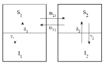
Figure 3: The system where the infected are prevented from migrating.

4.1 Equilibria

In addition to the origin, we find also the following two pairs of equilibria, $Z_{1}^{\pm}=(\tilde{S_{1}},\tilde{I_{1}},\tilde{S_{2}}^{\pm},0)$, $Z_{2}^{\pm}=(\tilde{S_{1}}^{\pm},0,\tilde{S_{2}},\tilde{I_{2}})$. At $Z_{1}$ the population values can be explicitly calculated,

$$\tilde{S_{1}}=\frac{\delta_{1}+\mu_{1}}{\gamma_{1}},\quad\tilde{I_{1}}=\tilde{S_{1}}\frac{r_{1}}{\mu_{1}}+\frac{r_{2}\tilde{S_{2}}}{\mu_{1}},\quad\tilde{S_{2}}^{\pm}=\frac{\ell\pm\sqrt{\ell^{2}-4r_{2}m_{21}A\tilde{S_{1}}(A+\tilde{S_{1}})}}{2r_{2}(A+\tilde{S_{1}})}$$

where $\ell=m_{12}A+m_{12}\tilde{S_{1}}-r_{2}A^{2}-r_{2}A\tilde{S_{1}}-m_{21}\tilde{S_{1}}$. These points are feasible if and only if

$$m_{21}\tilde{S_{1}}+r_{2}A^{2}+r_{2}A\tilde{S_{1}}<m_{12}A+m_{12}\tilde{S_{1}}.$$ (17)

The inequality is strict since for $\ell=0$ the corresponding quadratic equation has purely imaginary solutions. We also find at $Z_{2}$ the populations

$$\tilde{S_{2}}=\frac{\delta_{2}+\mu_{2}}{\gamma_{2}},\quad\tilde{I_{2}}=r_{2}\frac{\delta_{2}+\mu_{2}}{\gamma_{2}\mu_{2}}+\frac{r_{1}\tilde{S_{1}}}{\mu_{2}},\quad\tilde{S}_{1}^{\pm}=\frac{h\pm\sqrt{h^{2}-4r_{1}m_{12}A\tilde{S_{2}}(A+\tilde{S_{2}})}}{2r_{1}(A+\tilde{S_{2}})}$$

with $h=m_{21}A+m_{21}\tilde{S_{2}}-m_{12}\tilde{S_{2}}-r_{1}A^{2}-r_{1}A\tilde{S_{2}}$. Once again, noting the strict inequality, these equilibria are feasible if and only if

$$m_{12}\tilde{S_{2}}+r_{1}A^{2}+r_{1}A\tilde{S_{2}}<m_{21}A+m_{21}\tilde{S_{2}}.$$ (18)

Also the endemic coexistence equilibrium can be analytically evaluated,

$$\tilde{S_{1}}=\frac{\delta_{1}+\mu_{1}}{\gamma_{1}},\quad\tilde{I_{2}}=\frac{r_{1}\gamma_{2}(\delta_{1}+\mu_{1})+r_{2}\gamma_{1}(\delta_{2}+\mu_{2})-\tilde{I_{1}}\gamma_{1}\gamma_{2}\mu_{1}}{\gamma_{1}\gamma_{2}\mu_{2}},$$

$$\tilde{S_{2}}=\frac{\delta_{2}+\mu_{2}}{\gamma_{2}},\quad\tilde{I_{1}}=\frac{1}{\gamma_{1}\tilde{S_{1}}-\delta_{1}}\left[r_{1}\tilde{S_{1}}-m_{21}\frac{\tilde{S_{1}}}{A+\tilde{S_{1}}}+m_{12}\frac{\tilde{S}_{2}}{A+\tilde{S_{2}}}\right]$$

For feasibility, note that the denominator in the expression for $\tilde{I}_{1}$ reduces to $\mu_{1}$. Then $I_{1}\geq 0$ gives

$$r_{1}\tilde{S_{1}}+m_{12}\frac{\tilde{S}_{2}}{A+\tilde{S_{2}}}\geq m_{21}\frac{\tilde{S_{1}}}{A+\tilde{S_{1}}}.$$ (19)

We need also $I_{2}\geq 0$ i.e.

$$\tilde{I_{1}}\leq\frac{r_{1}\gamma_{2}(\delta_{1}+\mu_{1})+r_{2}\gamma_{1}(\delta_{2}+\mu_{2})}{\gamma_{1}\gamma_{2}\mu_{1}}$$ (20)

which can be recast in the following form

$$r_{2}\tilde{S_{2}}+m_{21}\frac{\tilde{S_{1}}}{A+\tilde{S_{1}}}\geq m_{12}\frac{\tilde{S}_{2}}{A+\tilde{S_{2}}}.$$ (21)

4.2 Stability

At the origin, the Jacobian has the explicit eigenvalues $\lambda_{1}=-\delta_{1}-\mu_{1}$, $\lambda_{2}=-\delta_{2}-\mu_{2}$ and the roots of the quadratic (8) so that the same analysis carries out also in this case, showing the inconditionate instability of this equilibrium point.

At $Z_{1}$ one eigenvalue is $\lambda_{1}=\gamma_{2}\tilde{S_{2}}-\delta_{2}-\mu_{2}$. The remaining ones are the roots of the cubic equation $\lambda^{3}+\hat{p_{2}}\lambda^{2}+\hat{p_{1}}\lambda+\hat{p_{0}}=0$ with

$$\hat{p_{2}}=\gamma_{1}\tilde{I_{1}}-r_{2}-r_{1}+\tilde{\eta_{1}}-\tilde{\eta_{2}}\tilde{S_{1}}+\tilde{\theta_{1}}-\tilde{\theta_{2}}\tilde{S_{2}}-\gamma_{1}\tilde{S_{1}}+\delta_{1}+\mu_{1},$$

$$\hat{p_{1}}=\gamma_{1}\tilde{I_{1}}(\gamma_{1}\tilde{S_{1}}-\delta_{1})+(\tilde{\theta_{1}}-\tilde{\theta_{2}}\tilde{S_{2}})(\gamma_{1}\tilde{I_{1}}-r_{1}-\gamma_{1}\tilde{S_{1}}+\delta_{1}+\mu_{1})$$

$$+(\tilde{\eta_{1}}\tilde{S_{1}}+r_{1}-\gamma_{1}\tilde{I_{1}}-\tilde{\eta_{1}})(r_{2}+\gamma_{1}\tilde{S_{1}}-\delta_{1}-\mu_{1})+r_{2}(\gamma_{1}\tilde{S_{1}}-\delta_{1}-\mu_{1}),$$

$$\hat{p_{0}}=\gamma_{1}\tilde{I_{1}}(\gamma_{1}\tilde{S_{1}}-\delta_{1})(\tilde{\theta_{1}}-\tilde{\theta_{2}}\tilde{S_{2}}-r_{2})-(\gamma_{1}\tilde{S_{1}}-\delta_{1}-\mu_{1})[r_{2}(\tilde{\eta_{2}}\tilde{S_{1}}$$

$$+r_{1}-\gamma_{1}\tilde{I_{1}}-\tilde{\eta_{1}})+(\gamma_{1}\tilde{I_{1}}-r_{1})(\tilde{\theta_{1}}-\tilde{\theta_{2}}\tilde{S_{2}})].$$

The Routh-Hurwitz conditions combined with negativity of the explicit eigenvalue ensure then stability:

$$\gamma_{2}\tilde{S_{2}}<\delta_{2}+\mu_{2},\quad\hat{p_{0}}>0,\quad\hat{p_{2}}>0,\quad\hat{p_{2}}\hat{p_{1}}>\hat{p_{0}}.$$ (22)

A similar situation arises for $Z_{2}$, one eigenvalue is found analytically, $\lambda_{1}=\gamma_{1}\tilde{S_{1}}-\delta_{1}-\mu_{1}$ and the cubic equation $\lambda^{3}+\hat{q_{2}}\lambda^{2}+\hat{q_{1}}\lambda+\hat{q_{0}}=0$ with coefficients

$$\hat{q_{2}}=-r_{2}-r_{1}+\gamma_{2}\tilde{I_{2}}+\tilde{\theta_{1}}-\tilde{\theta_{2}}\tilde{S_{2}}+\tilde{\eta_{1}}-\tilde{\eta_{2}}\tilde{S_{1}}-\gamma_{2}\tilde{S_{2}}+\delta_{2}+\mu_{2}$$

$$\hat{q_{1}}=-\gamma_{2}\tilde{I_{2}}(-\gamma_{2}\tilde{S_{2}}+\delta_{2})+(-\tilde{\eta_{1}}+\tilde{\eta_{2}}\tilde{S_{1}})(-\gamma_{2}\tilde{I_{2}}+r_{2}+\gamma_{2}\tilde{S_{2}}-\delta_{2}-\mu_{2})$$

$$+(-\gamma_{2}\tilde{I_{2}}-\tilde{\theta_{1}}+\tilde{\theta_{1}}\tilde{S_{2}}+r_{2})(r_{1}+\gamma_{2}\tilde{S_{2}}-\delta_{2}-\mu_{2})++r_{1}(\gamma_{2}\tilde{S_{2}}-\delta_{2}-\mu_{2})$$

$$\hat{q_{0}}=\gamma_{2}\tilde{I_{2}}(-\gamma_{2}\tilde{S_{2}}+\delta_{2})(-\tilde{\eta_{1}}+\tilde{\eta_{2}}\tilde{S_{1}}+r_{1})-(\gamma_{2}\tilde{S_{2}}-\delta_{2}-\mu_{2})[r_{1}(-\gamma_{2}\tilde{I_{2}}+$$

$$-\tilde{\theta_{1}}+\tilde{\theta_{2}}\tilde{S_{2}}+r_{2})+(-\gamma_{2}\tilde{I_{2}}+r_{2})(-\tilde{\eta_{1}}+\tilde{\eta_{2}}\tilde{S_{1}})]$$

for which the stability criterion becomes

$$\gamma_{1}\tilde{S_{1}}<\delta_{1}+\mu_{1},\quad\hat{q_{0}}>0,\quad\hat{q_{2}}>0,\quad\hat{q_{2}}\hat{q_{1}}>\hat{q_{0}}$$ (23)

Remark 1.

No bifurcations can arise here near the origin. The proof of this statement is exactly the same as the one carried out in Section 2.3.

The stability conditions for both equilibria $Z_{1}$ and $Z_{2}$ are nonempty, as can be easily shown numerically using respectively the following sets of parameters

$$r_{1}=1,\quad r_{2}=0.8,\quad\gamma_{1}=0.5,\quad\gamma_{2}=1,\quad\delta_{1}=1,\quad\delta_{2}=4,$$

$$\mu_{1}=1,\quad\mu_{2}=2,\quad m_{21}=2,\quad m_{12}=10,\quad A=5.$$

and

$$r_{1}=0.8,\quad r_{2}=1,\quad\gamma_{1}=1,\quad\gamma_{2}=0.5,\quad\delta_{1}=4,\quad\delta_{2}=1,$$

$$\mu_{1}=2,\quad\mu_{2}=1,\quad m_{21}=9,\quad m_{12}=2,\quad A=5.$$

The endemic equilibrium with all patches populated can numerically be shown to be attained for instance for the parameter values

$$r_{1}=1,\quad r_{2}=1,\quad\gamma_{1}=1,\quad\gamma_{2}=1,\quad\delta_{1}=0.5,\quad\delta_{2}=0.5,$$

$$\mu_{1}=1,\quad\mu_{2}=1,\quad m_{12}=1,\quad m_{21}=1,\quad A=1.$$

5 Biological Interpretation

For the general model, the system can never be wiped out, since the origin is unconditionally unstable. The ecosystem thrives with a nonvanishing population and an endemic state of the disease in both patches at stable levels, for certain parameter ranges.

These results hold true also for the particular case in which migrations back into patch 1 are forbidden. But in such case new possible equilibria arise, in which patch 1 is depleted, or in which only the susceptible population survives. But the latter equilibrium is never stable. The equilibrium with patch 1 empty is stable if the reproductive rate in that patch is low enough, or better, if the emigration rate is sufficiently high, compare (12). For the equilibrium with endemic disease and both patches populated, stability conditions have been derived, and the presence of a regime of possible oscillatory behavior has been highlighted.

If the infected do not migrate, once again the ecosystem is guaranteed to survive, as the origin is always unstable. The equilibria $Z_{1}$ and $Z_{2}$ are interesting, as in them one patch becomes disease-free. This is a result that potentially could be exploited by the manager of wild parks, to preserve at least part of a population from an epidemics. In order to control the disease at least in part of the environment it therefore appears to be better to preserve population movements in both directions, by preventing the infected to migrate, than to impose unidirectional migrations for both classes of individuals.

Acknowledgments.

The authors have been partially supported by the project “Metodi numerici in teoria delle popolazioni” of the Dipartimento di Matematica “Giuseppe Peano”.

References

• [1] Aimar, V., Borlengo, S., Motto, S., Venturino, E., A meta-epidemic model with steady state demographics and migrations saturation, AIP Conf. Proc. 1479, ICNAAM 2012, T. Simos, G. Psihoylos, Ch. Tsitouras, Z. Anastassi (Editors), 1311–1314 (2012); doi: 10.1063/1.4756396
• [2] Allen, L. J. S., Bolker, B. M., Lou, Y., Nevai, A. L., Asymptotic Profiles of the Steady States for an SIS Epidemic Patch Model, SIAM J. Appl. Math. 67, 1283–1309, (2007)
• [3] Arino, J., van den Driessche , P., Disease spread in metapopulations, Nonlinear Dynamics and Evolution Equations, Fields Inst. Commun. 48, H. Brunner, X. O. Zhao, and X. Zou, eds., AMS, Providence, RI, 1–13, (2006).
• [4] Arrigoni, F., Pugliese, A., Limits of a multi-patch SIS epidemic model, J. Math. Biol. 45, 419–440 (2002)
• [5] Barengo, M., Iennaco, I., Venturino, E., A simple meta-epidemic model, Proceedings of the 12th International Conference on Computational and Mathematical Methods in Science and Engineering, CMMSE 2012, J. Vigo-Aguiar, A.P. Buslaev, A. Cordero, M. Demiralp, I.P. Hamilton, E. Jeannot, V.V. Kozlov, M.T. Monteiro, J.J. Moreno, J.C. Reboredo, P. Schwerdtfeger, N. Stollenwerk, J.R. Torregrosa, E. Venturino, J. Whiteman (Editors) La Manga, Spain, July 2nd-5th, 2012, v. 1, p. 122–133 (2012)
• [6] Bianco, F., Cagliero, E., Gastelurrutia, M., Venturino, E., Metaecoepidemics with migration of and disease in the predators, Proceedings of the 11th International Conference on Computational and Mathematical Methods in Science and Engineering, CMMSE 2011, J. Vigo Aguiar, R. Cortina, S. Gray, J.M. Ferradiz, A. Fernandez, I. Hamilton, J.A. Lopez-Ramos, F. de Oliveira, R. Steinwandt, E. Venturino, J. Whiteman, B. Wade (Editors), Benidorm, Spain, June 26th-30th, v. 1, 204–223 (2011)
• [7] Gao, D., Ruan, S., An SIS patch model with variable transmission coefficients, Mathematical Biosciences 232, 110–115 (2011)
• [8] Hanski, I., Gilpin, M., Metapopulation biology: ecology, genetics and evolution, London: Academic Press (1997)
• [9] Jin, Y., Wang, W., The effect of population dispersal on the spread of a disease, J. Math. Anal. Appl. 308, 343–364 (2005)
• [10] Lloyd, A., May, R. M., Spatial heterogeneity in epidemic models, J. Theoret. Biol. 179, 1–11 (1996)
• [11] Malchow, H., Petrovskii, S., Venturino, E., Spatiotemporal patterns in Ecology and Epidemiology. CRC, Boca Raton (2008)
• [12] Salmani, M., van den Driessche, P., A model for disease transmission in a patchy environment, Discrete Contin. Dynam. Systems Ser. B 6, 185–202 (2006)
• [13] Venturino, E., Simple metaecoepidemic models, Bull. Math. Biol. 73, 917–950 (2011)
• [14] Wang, W., Population dispersal and disease spread, Discrete Contin. Dynam. Systems Ser. B 4, 797–804 (2004)
• [15] Wang, W., Mulone, G., Threshold of disease transmission in a patch environment, J. Math. Anal. Appl. 285, 321–335 (2003)
• [16] Wang, W.. Ruan, S., Simulating the SARS outbreak in Beijing with limited data, J. Theoret. Biol. 227, 369–379 (2004)
• [17] Wang, W., Zhao, X.-Q., An epidemic model in a patchy environment, Math. Biosci. 190, 97–112 (2004)
• [18] Wiens, J. A., Wildlife in patchy environments: metapopulations, mosaics, and management, in D. R. McCullough (Ed.) Metapopulations and Wildlife Conservation. Island Press, Washington 53–84 (1996)
• [19] Wiens, J. A., Metapopulation dynamics and landscape ecology, in I. A. Hanski, M. E. Gilpin (Ed.s), 43–62. Academic Press, San Diego, (1997)