Frozen density embedding with non-integer subsystems’ particle numbers

Abstract

We extend the frozen density embedding theory to non-integer subsystems’ particles numbers. Different features of this formulation are discussed, with special concern for approximate embedding calculations. In particular, we highlight the relation between the non-integer particle-number partition scheme and the resulting embedding errors. Finally, we provide a discussion of the implications of the present theory for the derivative discontinuity issue and the calculation of chemical reactivity descriptors.

I Introduction

Subsystem approaches Senatore and Subbaswamy (1986); Cortona (1991); Yang (1991); Cortona and Monteleone (1994); Yang and Lee (1995); ichirou Sugiki et al. (2003); Fedorov and Kitaura (2004); Huang and Carter (2006); Wesolowski (2006); Cohen and Wasserman (2007); Cohen et al. (2007); Akama et al. (2007); Wang et al. (2008); Zhao et al. (2008); He et al. (2009); Elliott et al. (2010); Huang and Carter (2011); huang11_2 ; Gordon et al. (2012); Severo Pereira Gomes and Jacob (2012); Manby et al. (2012); Wesolowski and Wang (2013) are powerful tools in the context of density functional theory Hohenberg and Kohn (1964); Parr and Yang (1989). In particular, the frozen density embedding (FDE) theory and its related methods Senatore and Subbaswamy (1986); Cortona (1991); Wesolowski (2006); Wesolowski and Warshel (1993); Neugebauer et al. (2005a); Jacob et al. (2006, 2008); Wesołowski (2008); Neugebauer (2009a); Laricchia et al. (2010); Kaminski et al. (2010); Fux et al. (2010); owski (2011); Fux et al. (2011); Pavanello and Neugebauer (2011); Laricchia et al. (2011a); Aquilante and owski (2011); de Silva and Wesolowski (2012); Laricchia et al. (2012); jacobrev , emerged in the last years as simple and powerful approaches to treat, in an in principle exact manner, non-covalent complexes Jacob et al. (2006); Pavanello and Neugebauer (2011); Neugebauer et al. (2005b); Jacob et al. (2005); Kevorkyants et al. (2006); Dulak and Wesolowski (2007); Dulak et al. (2007); Neugebauer (2009b); Götz et al. (2009); Kaminski et al. (2010); Constantin et al. (2011); Laricchia et al. (2011b); Fradelos and Wesołowski (2011); Fradelos et al. (2011); Laricchia et al. (2012, 2013).

Within the FDE method the electron density is partitioned into several subsystem’s contributions that are constrained to sum up to the total electron density. The ground-state density is then obtained by minimizing the total energy of the system with respect to one of the subsystem’s densities keeping the other ones fixed (i.e., frozen). In this way, in principle, the full solution of the Hohenberg-Kohn variational problem Hohenberg and Kohn (1964) is obtained. If auxiliary orbitals are introduced to expand the electron density, the FDE problem can be recast into the familiar framework of the Kohn-Sham (KS) method Kohn and Sham (1965). In this case the ground-state solution is given by a set of coupled KS equations with constrained electron density (KSCED) Wesolowski and Warshel (1993).

The partition of the density, which is at the base of the FDE procedure, is in principle arbitrary and any convenient choice can be made for the system under examination. However, the actual formalism of the FDE theory, both in the orbital-free and the orbital-based formulation, is founded on a pure-state representation of the electron densities. Therefore, only subsystem densities with integer number of electrons are allowed. The integer occupation of subsystems limits the choice of possible frozen densities and, in addition, has important consequences from a more formal point of view. In fact, non-integer particle numbers have been shown to be of extreme importance for the deep comprehension and the development of density functional theory Perdew et al. (1982); Janak (1978); Yang et al. (2012); Cohen et al. (2012, 2008a, 2008b); Fabiano and Constantin (2013). In particular, we mention the fact that the use of non-integer numbers of particles is intrinsically related to the fundamental issue of the derivative discontinuity of density functional theory Perdew et al. (1982); Cohen et al. (2012) and stands at the basis of all definitions in chemical reactivity theory Cohen and Wasserman (2007); Parr and Yang (1989); Chattaraj (2009); Chermette (1999); Geerlings et al. (2003). In addition, concerning this latter aspect, Ref. Cohen and Wasserman (2007) showed the importance of both non-integer occupations and environmental effects for a proper definition of chemical descriptors. Thus, in order to be able to have deep insight into the fundamental properties of the embedding potential or access chemical reactivity descriptors for the embedded subsystems via the FDE approach, it is necessary to have a proper FDE theory for non-integer particle numbers.

We acknowledge that other embedding theories exist where non-integer particle numbers are allowed Elliott et al. (2010); Huang and Carter (2011); huang11_2 ; Elliott et al. (2009); Tang et al. (2012). Namely, the partition density-functional theory (PDFT) Elliott et al. (2010, 2009) and the potential-functional embedding theory of Huang and Carter Huang and Carter (2011); huang11_2 . The latter is not a density-based theory, since the total electronic energy is formulated as a functional of the embedding potential rather than of the subsystems’ densities. Moreover, in both cases no frozen density is considered but the solution is found by variational minimization of all the subsystems’ densities and particle numbers. Thus, the non-integer occupation of a given subsystem cannot be considered as a parameter inherent with the chosen partition scheme, as in FDE, but it is automatically determined by the self-consistent solution of the embedding problem. Furthermore, we note that the minimization of the total electronic energy with respect to the subsystems’ occupations may arise some conceptual problems in practical calculations where an approximate density functional is employed for the kinetic energy, because the true and approximate energy functionals may be minimized by different sets of occupation numbers mosquera13 .

In this paper we focus on the FDE formalism and consider its extension to non-integer subsystems’ particle numbers, by considering a zero-temperature grand-canonical ensemble formalism Perdew et al. (1982). The implications of the developed theory are then discussed to highlight the significance of non-integer subsystems’ particle numbers, especially in approximate embedding calculations. Furthermore, we shortly comment on the relevance of the present approach for the comprehension of the role of the derivative discontinuity in the FDE context as well as for the definition of well-posed chemical descriptors for embedded subsystems.

II Frozen density embedding with ensemble subsystem densities

Within the Levy’s constrained search Levy (1979); Lieb (1983) it is well established that the ground-state energy of any $N$-electron system can be expressed as

$$E_{0}=\min_{\rho\rightarrow N}\left\{\min_{\Psi\rightarrow\rho}\braket{\Psi}{\hat{T}+\hat{V}_{ee}}{\Psi}+\int\rho(\mathbf{r})v_{\text{ext}}(\mathbf{r})d\mathbf{r}\right\}\ ,$$ (1)

where $N$ is any integer number, $\rho$ is an $N-$representable electron density, $\Psi$ is an $N$-particle wave function yielding the density $\rho$, $\hat{T}$ is the kinetic energy operator, $\hat{V}_{ee}$ is the electron-electron interaction operator, and $v_{\text{ext}}$ is an external potential (usually the nuclear potential). The functional

$$F[\rho]=\min_{\Psi\rightarrow\rho}\braket{\Psi}{\hat{T}+\hat{V}_{ee}}{\Psi}$$ (2)

is called the Hohenberg-Kohn universal functional and its existence is guaranteed by the first theorem of Hohenberg and Kohn Hohenberg and Kohn (1964).

Now we consider a partitioning of the density into $\rho=\rho_{A\omega}+\rho_{B\omega}$, where $\rho_{A\omega}$ and $\rho_{B\omega}$ are the ensemble $(N_{A}+\omega)$- and $(N_{B}-\omega)$-representable electron densities

$$\rho_{A\omega}=\mathrm{Tr\left[\hat{\Gamma}_{A\omega}\hat{\rho}\right]}\quad;\quad\rho_{B\omega}=\mathrm{Tr\left[\hat{\Gamma}_{B\omega}\hat{\rho}\right]}\ .$$ (3)

Here $N_{A}$ and $N_{B}$ are two integer numbers such that $N_{A}+N_{B}=N$, $\omega\in[-1,1]$, $\hat{\rho}$ is the density operator in second quantization representation, and

$$\hat{\Gamma}_{A\omega}=\pm\omega|\Psi_{A,N_{A}\pm 1}\rangle\langle\Psi_{A,N_{A}\pm 1}|+(1\mp\omega)|\Psi_{A,N_{A}}\rangle\langle\Psi_{A,N_{A}}|$$ (4)

$$\hat{\Gamma}_{B\omega}=\pm\omega|\Psi_{B,N_{B}\mp 1}\rangle\langle\Psi_{B,N_{B}\mp 1}|+(1\mp\omega)|\Psi_{B,N_{B}}\rangle\langle\Psi_{B,N_{B}}|$$ (5)

are the density operators describing the subsystems $A$ and $B$, respectively, with $\Psi_{i,M}$ being an $M$-electron wave function for subsystem $i$ and the upper and lower signs in $\pm$ and $\mp$ corresponding to $\omega>0$ and $\omega<0$ respectively. Furthermore, we assume that $\rho_{B\omega}$ is fixed to some given trial value respecting minimal conditions for a physical subsystem density (see subsection II.2).

According to our partition scheme we define the following functionals

$$F[\rho_{A\omega}]=\min_{\hat{\Gamma}_{A\omega}\rightarrow\rho_{A\omega}}\mathrm{Tr\left[\hat{\Gamma}_{A\omega}\left(\hat{T}+\hat{V}_{ee}\right)\right]}$$ (6)

$$F[\rho_{B\omega}]=\min_{\hat{\Gamma}_{B\omega}\rightarrow\rho_{B\omega}}\mathrm{Tr\left[\hat{\Gamma}_{B\omega}\left(\hat{T}+\hat{V}_{ee}\right)\right]}$$ (7)

$$F^{nadd}[\rho_{A\omega},\rho_{B\omega}]=F[\rho_{A\omega}+\rho_{B\omega}]-F[\rho_{A\omega}]-F[\rho_{B\omega}]\ ,$$ (8)

where $F[\rho_{A\omega}+\rho_{B\omega}]=F[\rho]$ is independent from $\omega$ and is given by Eq. (2). The ground-state energy of Eq. (1) can be thus written

$$E_{0} = \min_{\rho_{A\omega}\rightarrow N_{A}+\omega}\biggl{\{}F[\rho_{A\omega}]+F[\rho_{B\omega}]+F^{nadd}[\rho_{A\omega},\rho_{B\omega}]$$ (9)

$$+\int\left[\rho_{A\omega}(\mathbf{r})+\rho_{B\omega}(\mathbf{r})\right]v_{\text{ext}}(\mathbf{r})d\mathbf{r}\biggr{\}}\ ,$$

where the minimization over $\rho$ was substituted by the minimization over $\rho_{A\omega}$ in consideration of the fact that $\rho_{B\omega}$ is fixed. Note that Eq. (9) is in fact fully equivalent to Eq. (1), despite the fact that $\rho_{B\omega}$ and $\omega$ are arbitrarily fixed, because it always admits the formal solution $\rho_{A\omega}^{min}=\rho^{min}-\rho_{B\omega}$, where $\rho^{min}$ is the density minimizing Eq. (1) Wesolowski (2006).

According to Eq. (9), we have to minimize the functional

$$\mathscr{L}[\rho_{A\omega}] = F[\rho_{A\omega}]+F[\rho_{B\omega}]+F^{nadd}[\rho_{A\omega},\rho_{B\omega}]$$

$$+ \int\left[\rho_{A\omega}(\mathbf{r})+\rho_{B\omega}(\mathbf{r})\right]v_{\text{ext}}(\mathbf{r})d\mathbf{r}$$

$$- \mu\left(\int\mathrm{Tr\left[\hat{\Gamma}_{A\omega}\hat{\rho}\right]}d\mathbf{r}-N_{A}-\omega\right)\ ,$$

where $\mu$ is the Lagrange multiplier associated with the condition $\rho_{A\omega}\rightarrow N_{A}+\omega$. To minimize the functional $\mathscr{L}$ we consider a small variation of the density operator $\hat{\Gamma}_{A\omega}\rightarrow\hat{\Gamma}_{A\omega}+\delta\hat{\Gamma}_{A\omega}$ so that $\rho_{A\omega}\rightarrow\rho_{A\omega}+\delta\rho_{A\omega}$ with $\delta\rho_{A\omega}=\mathrm{Tr\left[\delta\hat{\Gamma}_{A\omega}\hat{\rho}\right]}$. Thus, retaining only the first-order terms, we obtain

$$\int\left(\frac{\delta F[\rho_{A\omega}]}{\delta\rho_{A\omega}(\mathbf{r})}+\frac{\delta F^{nadd}[\rho_{A\omega},\rho_{B\omega}]}{\delta\rho_{A\omega}(\mathbf{r})}+v_{\text{ext}}(\mathbf{r})-\mu\right)\delta\rho_{A\omega}(\mathbf{r})d\mathbf{r}=0\ ,$$ (11)

which yields the Euler equation

$$\frac{\delta F[\rho_{A\omega}]}{\delta\rho_{A\omega}(\mathbf{r})}+\frac{\delta F^{nadd}[\rho_{A\omega},\rho_{B\omega}]}{\delta\rho_{A\omega}(\mathbf{r})}+v_{ext}(\mathbf{r})=\mu\ .$$ (12)

If we partition the external potential as $v_{\text{ext}}=v_{\text{ext}}^{A}+v_{\text{ext}}^{B}$, we can finally write

$$\frac{\delta F[\rho_{A\omega}]}{\delta\rho_{A\omega}(\mathbf{r})}+v_{\text{ext}}^{A}(\mathbf{r})+v_{emb}^{A}[\rho_{A\omega};\rho_{B\omega}](\mathbf{r})=\mu\ ,$$ (13)

where we defined

$$v_{emb}^{A}[\rho_{A\omega};\rho_{B\omega}](\mathbf{r})\equiv\frac{\delta F^{nadd}[\rho_{A\omega},\rho_{B\omega}]}{\delta\rho_{A\omega}(\mathbf{r})}+v_{\text{ext}}^{B}(\mathbf{r})\ .$$ (14)

The embedding potential $v_{emb}^{A}$ is therefore the external potential needed to constrain the solution of the subsystem $A$ to yield the electron density of the total system through the condition $\rho=\rho_{A\omega}+\rho_{B\omega}$.

II.1 Kohn-Sham formulation

To develop a Kohn-Sham formulation for our problem we introduce, for each value of $\omega$, a reference ensemble non-interacting system with external potential $w$ such that the ensemble non-interacting and interacting densities are the same. According to Eq. (4), such a system is described by the density operator

$$\hat{\Gamma}_{A\omega}^{KS}=\pm\omega|\Phi^{(\omega)}_{A,N_{A}\pm 1}\rangle\langle\Phi^{(\omega)}_{A,N_{A}\pm 1}|+(1\mp\omega)|\Phi^{(\omega)}_{A,N_{A}}\rangle\langle\Phi^{(\omega)}_{A,N_{A}}|\ ,$$ (15)

where $\langle\mathbf{r}_{1}\ldots\mathbf{r}_{M}|\Phi^{(\omega)}_{A,M}\rangle$ is an $M$-particle Slater determinant, depending implicitly on $\omega$ (for each value of $\omega$ a different external potential $w$ will be needed to guarantee the equality of the ensemble non-interacting and interacting densities; throughout the paper the superscript ^(ω) will be used to denote this implicit dependence). Thus, the reference system has a non-interacting kinetic energy

$$T_{s}[\rho_{A\omega}]=\min_{\hat{\Gamma}^{KS}_{A\omega}\rightarrow\rho_{A\omega}}\mathrm{Tr\left[\hat{\Gamma}^{KS}_{A\omega}\hat{T}\right]}$$ (16)

and its ground state is described by the Euler equation

$$\frac{\delta T_{s}[\rho_{A\omega}]}{\delta\rho_{A\omega}(\mathbf{r})}+w(\mathbf{r})=\mu\ .$$ (17)

Comparison of Eqs. (13) and (17) allows to identify $w(\mathbf{r})=v_{s}^{A}(\mathbf{r})+v_{emb}^{A}(\mathbf{r})$ where we defined the KS potential

$$v_{s}^{A}(\mathbf{r})=\int\frac{\rho_{A\omega}(\mathbf{r}_{1})}{|\mathbf{r}-\mathbf{r}_{1}|}d\mathbf{r}_{1}+\frac{\delta E_{xc}[\rho_{A\omega}]}{\delta\rho_{A\omega}(\mathbf{r})}+v_{\text{ext}}^{A}(\mathbf{r})\ ,$$ (18)

with $E_{xc}[\rho_{A\omega}]=F[\rho_{A\omega}]-T_{s}[\rho_{A\omega}]-J[\rho_{A\omega}]$ and $J$ the classical Coulomb energy.

Practical equations for ground-state calculations are obtained considering that the KS Slater determinants entering in Eq. (15) are constructed with orbitals that are solutions of the Schrödinger equation for a single particle in an external potential $w$. Thus, the ground-state for subsystem $A$ is given by the KSCED

$$\left(-\frac{1}{2}\nabla^{2}+v^{A}_{s}[\rho_{A\omega}]+v_{emb}^{A}[\rho_{A\omega};\rho_{B\omega}]\right)\phi^{(\omega)}_{A,i}=\epsilon^{(\omega)}_{A,i}\phi^{(\omega)}_{A,i}\ ,$$ (19)

with the electron density computed as

$$\rho_{A\omega}=\mathrm{Tr\left[\hat{\Gamma}^{KS}_{A\omega}\hat{\rho}\right]}=\sum_{i}f_{i}|\phi_{A,i}^{(\omega)}|^{2}\ ,$$ (20)

where the occupation numbers are

$$f_{i} = \left\{\begin{array}[]{lc}1&i\leq N_{A}\\ \omega&i=N_{A}+1\\ 0&i>N_{A}+1\\ \end{array}\right.\ \ \mathrm{for}\ \omega>0\quad;$$ (24)

$$f_{i} = \left\{\begin{array}[]{lc}1&i\leq N_{A}-1\\ 1+\omega&i=N_{A}\\ 0&i>N_{A}\\ \end{array}\right.\ \ \mathrm{for}\ \omega<0\ .$$ (28)

In the KS scheme introduced above the embedding potential of Eq. (14) can be recast into a more practical form by writing

$$v_{emb}^{A}[\rho_{A\omega};\rho_{B\omega}](\mathbf{r}) = v_{\text{ext}}^{B}(\mathbf{r})+\int\frac{\rho_{B\omega}(\mathbf{r}_{1})}{|\mathbf{r}-\mathbf{r}_{1}|}d\mathbf{r}_{1}$$

$$+ \frac{\delta T^{nadd}_{s}[\rho_{A\omega};\rho_{B\omega}]}{\delta\rho_{A\omega}(\mathbf{r})}+\frac{\delta E^{nadd}_{xc}[\rho_{A\omega};\rho_{B\omega}]}{\delta\rho_{A\omega}(\mathbf{r})}\ ,$$

where

$$T^{nadd}_{s}[\rho_{A\omega};\rho_{B\omega}]=T_{s}[\rho_{A\omega}+\rho_{B\omega}]-T_{s}[\rho_{A\omega}]-T_{s}[\rho_{B\omega}]$$

$$E^{nadd}_{xc}[\rho_{A\omega};\rho_{B\omega}]=E_{xc}[\rho_{A\omega}+\rho_{B\omega}]-E_{xc}[\rho_{A\omega}]-E_{xc}[\rho_{B\omega}]$$

are the non-additive non-interacting kinetic and exchange-correlation energy functionals, respectively. Appropriate approximations must be used to express $T_{s}$ and $E_{xc}$ for practical calculations (see section II.3). In particular we note that, while the functionals $T_{s}[\rho_{A\omega}+\rho_{B\omega}]=T_{s}[\rho]$ and $E_{xc}[\rho_{A\omega}+\rho_{B\omega}]=E_{xc}[\rho]$ are defined for pure-state densities, so that conventional approximations Scuseria and Staroverov (2005); Wesolowski and Weber (1997); Götz et al. (2009); Laricchia et al. (2011b) can be employed straightforwardly, the functionals $T_{s}[\rho_{A\omega}]$ and $E_{xc}[\rho_{A\omega}]$ are defined for ensemble densities, thus special care may be needed in their approximation (see e.g. Refs. Ullrich and Kohn, 2001; Kraisler and Kronik, 2013).

II.2 Full self-consistent solution

In the previous sections we considered $\rho_{B\omega}$ fixed to any arbitrary function satisfying the minimal requirements for a physical subsystem density Parr and Yang (1989), i.e. everywhere we must have $0\leq\rho_{B\omega}\leq\rho$, $0<\int\rho_{B\omega}\,d\mathbf{r}<N$ and also $\int|\nabla\rho_{B\omega}^{1/2}|^{2}\,d\mathbf{r}<\infty$. In this way only $\rho_{A\omega}$ was variationally optimized to yield the full ground-state density. This condition, although it may result advantageous in some situations, leads to the problem of the choice of an optimal $\rho_{B\omega}$. In fact, even simple choices of $\rho_{B\omega}$ turn out to be problematic. For example, the use of the electron density of the isolated subsystem $B$ generally violates the condition $\rho_{B\omega}\leq\rho$ in some regions of space Kiewisch et al. (2008). Moreover, if the Kohn-Sham scheme is used for solution, as it is often the case, the frozen density must satisfy the additional condition that $\rho_{A\omega}=\rho-\rho_{B\omega}$ is a $v_{s}$-representable electron density, that means that it must be the ground-state associated with a KS potential. This condition is of course very hard to fulfill a priori, because the total density $\rho$ is not known in embedding calculations.

A failure of the frozen $\rho_{B\omega}$ to fulfill all the requirements described above, will prevent the embedding calculation to converge to the correct solution. Therefore, it may be preferable instead to determine both $\rho_{A\omega}$ and $\rho_{B\omega}$ through a variational procedure.

To this end we can reconsider Eq. (9) and write it as

$$E_{0} = \min_{\begin{subarray}{c}\rho_{A\omega}\rightarrow N_{A}+\omega\\ \rho_{B\omega}\rightarrow N_{B}-\omega\end{subarray}}\left\{F[\rho_{A\omega}]+F[\rho_{B\omega}]+F^{nadd}[\rho_{A\omega},\rho_{B\omega}]+\right.$$ (31)

$$\left.+\int\left[\rho_{A\omega}(\mathbf{r})+\rho_{B\omega}(\mathbf{r})\right]v_{\text{ext}}(\mathbf{r})d\mathbf{r}\right\}\ ,$$

where now the minimization involves both densities and must be constrained by the condition $N_{A}+N_{B}=N$. Thus, we have to minimize the functional

$$\mathscr{L}[\rho_{A\omega},\rho_{B\omega}]=F[\rho_{A\omega}]+F[\rho_{B\omega}]+F^{nadd}[\rho_{A\omega},\rho_{B\omega}]+$$

$$\quad+\int\left[\rho_{A\omega}(\mathbf{r})+\rho_{B\omega}(\mathbf{r})\right]v_{\text{ext}}(\mathbf{r})d\mathbf{r}-$$

$$\quad-\mu\left(\int\mathrm{Tr\left[\hat{\Gamma}_{A\omega}\hat{\rho}\right]}d\mathbf{r}+\int\mathrm{Tr\left[\hat{\Gamma}_{B\omega}\hat{\rho}\right]}d\mathbf{r}-N\right)\ ,$$ (32)

Following the steps bringing from Eq. (II) to Eq. (13) we finally find the set of coupled equations

$$\frac{\delta F[\rho_{A\omega}]}{\delta\rho_{A\omega}(\mathbf{r})}+v_{\text{ext}}^{A}(\mathbf{r})+v_{emb}^{A}[\rho_{A\omega};\rho_{B\omega}](\mathbf{r}) = \mu$$ (33)

$$\frac{\delta F[\rho_{B\omega}]}{\delta\rho_{B\omega}(\mathbf{r})}+v_{\text{ext}}^{B}(\mathbf{r})+v_{emb}^{B}[\rho_{B\omega};\rho_{A\omega}](\mathbf{r}) = \mu\ .$$ (34)

These equations, or the analogous set of KSCED, can be solved in a freeze-and-thaw scheme Wesolowski and Weber (1996) to yield a fully variational solution of the embedding problem.

Note however, that even though the densities are obtained through the solution of the coupled equations (33) and (34), we are still left with some arbitrarity in the choice of the subsystem densities. In fact, in Eq. (32) there is only a constraint on the total number of electrons, but no restrictions on the individual values of $N_{A}+\omega$ and $N_{B}-\omega$. Therefore, for any system there exists a family of fully variational exact embedding solutions $\rho_{A\omega}$ and $\rho_{B\omega}$ which provide exactly the same total ground-state energies and densities. Note that within the FDE theory, only the ground-state energy and density of the total system are meaningful, while the subsystems densities and energies are, in principle, not well (and uniquely) defined, unlike in PDFTElliott et al. (2010).

II.3 Comments on approximate frozen density embedding

In practical applications of the Kohn-Sham method the exchange-correlation (XC) energy (and the corresponding potential) need to be approximated, because the exact form of this term is not known. In the present paper and in most FDE applications only local/semilocal XC approximations are considered. These suffice in fact for various applications Fabiano et al. (2011); Goerigk and Grimme (2010). Moreover, they display an explicit dependence from the electron density. With this choice, the XC part of the embedding potential can be computed on the same level as the XC potential of the full KS calculation and no additional approximation is needed in the embedding calculations (for our purposes we can assume the XC approximation is used from the beginning in the construction of the Hohenberg-Kohn universal functional of Eq. (2)).

On the other hand, the non-interacting kinetic energy is treated exactly within the KS scheme, but it needs to be approximated in the embedding potential, since in this latter case we cannot make use of auxiliary orbitals for the total embedded system, but rather require an explicitly density-dependent functional (we remark that an alternative strategy based on the explicit construction of the kinetic potential using the numerical inversion procedures also exists Fux et al. (2010); de Silva and Wesolowski (2012), but is not applicable in practical calculations) . Thus, local or semilocal approximations are introduced for the non-additive kinetic energy in any practical calculation based on the frozen density embedding method. This approximation is the only source of errors in semilocal embedding calculations, when compared with the corresponding KS results for the whole system.

The inclusion of approximations in the embedding procedure has important consequences on the outcome of the embedding calculations Gritsenko (2013). The first, of course, is that the true ground-state energy and density cannot be recovered any more because Eqs. (1) and (9) (or (1) and (31)) minimize different functionals. More importantly, the final result of the embedding calculation is no more independent on the choice of the “frozen” density $\rho_{B\omega}$. In fact, while for the exact kinetic energy the functional in Eq. (9) is truly dependent only on the sum $\rho_{A\omega}+\rho_{B\omega}$, so that it will yield always the same result whenever the sum is left unchanged, for approximate kinetic energy functionals the functional of Eq. (9) really depends on $\rho_{A\omega}$ and $\rho_{B\omega}$ separately and will likely provide different results for different choices of $\rho_{B\omega}$. This problem can be naturally mitigated by employing a full self-consistent solution for the embedding densities, so that both $\rho_{A\omega}$ and $\rho_{B\omega}$ are provided as a solution of the coupled equations (33) and (34). However, as mentioned before, also in this case different solutions will be in general obtained for different choices of the charge partitioning scheme, i.e. for different values of $\omega$. The investigation of this dependence will be the main subject of the following sections.

III Effect of the non-integer particle numbers on the embedding density

Consider an ensemble $v_{s}$-representable frozen density $\rho_{B\omega}$ which integrates to the fractional occupation $N_{B}-\omega$ with $\omega\geq 0$ (the case $\omega<0$ is analogous and will not be explicitly considered in the following, except for the fact that some final formulas will be stated for both cases when needed). We assume that such a density can be written (which is valid also for a full self-consistent calculation)

$$\rho_{B\omega}=\omega\rho_{B,N_{B}-1}^{(\omega)}+(1-\omega)\rho_{B,N_{B}}^{(\omega)}\ ,$$ (35)

with the pure-state ($N_{B}-1$)- and $N_{B}$-electron densities defined as

$$\rho_{B,N_{B}-1}^{(\omega)}=\sum_{i}^{N_{B}-1}\left|\phi_{B,i}^{(\omega)}\right|^{2}\quad;\quad\rho_{B,N_{B}}^{(\omega)}=\sum_{i}^{N_{B}}\left|\phi_{B,i}^{(\omega)}\right|^{2}\ ,$$ (36)

where the $\phi_{B,i}^{(\omega)}$ are some orbitals solution of a single-particle equation of the form of Eq. (19). Of course, the frozen density can be also written in the alternative form given by Eqs. (20) and (24).

For an exact embedding calculation, the complementary subsystem density $\rho_{A\omega}$, with fractional occupation $N_{A}+\omega$ will be $\rho_{A\omega}=\rho^{KS}-\rho_{B\omega}$. This density is also ensemble $v_{s}$-representable. In fact, direct substitution of this density into Eqs. (18), (II.1), and (19) yields the equation

$$\left[-\frac{1}{2}\nabla^{2}+\frac{\delta T_{s}[\rho^{KS}]}{\delta\rho_{A\omega}}-\frac{\delta T_{s}[\rho_{A\omega}]}{\delta\rho_{A\omega}}+v_{s}^{KS}\right]\phi_{A,i}^{(\omega)}=\epsilon_{A,i}^{(\omega)}\phi_{A,i}^{(\omega)}\ ,$$ (37)

where $v_{s}^{KS}$ denotes the Kohn-Sham potential of the full system. The ($N_{A}+\omega$)-electron density constructed from the orbitals satisfying Eq. (37) is, by construction, the one that minimizes Eq. (17) (or equivalently Eq. (13)). Thus, it is by definition $\rho_{A\omega}=\rho^{KS}-\rho_{B\omega}$.

As described in Section II.1, the electron density of subsystem $A$ is given by Eqs. (20) and (24). Alternatively, we can write it as

$$\rho_{A\omega}=\omega\rho_{A,N_{A}+1}^{(\omega)}+(1-\omega)\rho_{A,N_{A}}^{(\omega)}\ ,$$ (38)

with the pure-state densities defined as

$$\rho_{A,N_{A}+1}^{(\omega)}=\sum_{i}^{N_{A}+1}\left|\phi_{A,i}^{(\omega)}\right|^{2}\quad;\quad\rho_{A,N_{A}}^{(\omega)}=\sum_{i}^{N_{A}}\left|\phi_{A,i}^{(\omega)}\right|^{2}\ .$$ (39)

Similar results hold also in the case of a full self-consistent FDE calculation, where both $\rho_{A\omega}$ and $\rho_{B\omega}$ are optimized variationally.

Using the definitions (35) and (38) we can readily write for the total embedding density

$$\rho_{A\omega}+\rho_{B\omega} = \rho_{A,N_{A}}^{(\omega)}+\rho_{B,N_{B}}^{(\omega)}+$$

$$+\omega\left(\rho_{A,N_{A}+1}^{(\omega)}-\rho_{A,N_{A}}^{(\omega)}+\rho_{B,N_{B}-1}^{(\omega)}-\rho_{B,N_{B}}^{(\omega)}\right)\ .$$

That is

$$\rho_{A\omega}+\rho_{B\omega}=\rho_{A,N_{A}}^{(\omega)}+\rho_{B,N_{B}}^{(\omega)}+\omega\left(\left|\phi_{A,N_{A}+1}^{(\omega)}\right|^{2}-\left|\phi_{B,N_{B}}^{(\omega)}\right|^{2}\right)\ .$$ (41)

Expanding the orbitals and densities in powers of $\omega$, i.e.

$$\phi_{i}^{(\omega)} \approx \phi_{i}^{(\omega=0)}+\omega\frac{\partial\phi_{i}^{(\omega)}}{\partial\omega}\Big{|}_{\omega=0^{+}}+\frac{\omega^{2}}{2}\frac{\partial^{2}\phi_{i}^{(\omega)}}{\partial\omega^{2}}\Big{|}_{\omega=0^{+}}+\cdots$$ (42)

$$\rho_{i}^{(\omega)} \approx \rho_{i}^{(\omega=0)}+\omega\frac{\partial\rho_{i}^{(\omega)}}{\partial\omega}\Big{|}_{\omega=0^{+}}+\frac{\omega^{2}}{2}\frac{\partial^{2}\rho_{i}^{(\omega)}}{\partial\omega^{2}}\Big{|}_{\omega=0^{+}}+\cdots\ ,$$ (43)

it is then possible to express the total embedding density as a power series in $\omega$

$$\rho_{A\omega}+\rho_{B\omega}=A_{0}+A_{1}^{+}\omega+A_{2}^{+}\omega^{2}+\cdots\ ,$$ (44)

where (up to second order)

$$A_{0} \equiv \rho_{A,N_{A}}^{(0)}+\rho_{B,N_{B}}^{(0)}$$ (45)

$$A_{1}^{+} \equiv \left|\phi_{A,N_{A}+1}^{(0)}\right|^{2}-\left|\phi_{B,N_{B}}^{(0)}\right|^{2}+\frac{\partial\left(\rho_{A,N_{A}}^{(\omega)}+\rho_{B,N_{B}}^{(\omega)}\right)}{\partial\omega}\Big{|}_{\omega=0^{+}}$$ (46)

$$A_{2}^{+} \equiv 2\phi_{A,N_{A}+1}^{(0)}\frac{\partial\phi_{A,N_{A}+1}^{(\omega)}}{\partial\omega}\Big{|}_{\omega=0^{+}}-$$

$$-2\phi_{B,N_{B}}^{(0)}\frac{\partial\phi_{B,N_{B}}^{(\omega)}}{\partial\omega}\Big{|}_{\omega=0^{+}}+\frac{\partial^{2}\left(\rho_{A,N_{A}}^{(\omega)}+\rho_{B,N_{B}}^{(\omega)}\right)}{\partial\omega^{2}}\Big{|}_{\omega=0^{+}}\ ,$$

and we have assumed real single-particle orbitals. The terms $A_{1}^{+}$, $A_{2}^{+}$ and higher include, through the derivatives of the densities and orbitals, the linear, quadratic and higher response of the embedded subsystems to a charge transfer $A\rightarrow B$. These are thus very complex terms (see also subsection III.1). Nevertheless, for the exact embedding we must have $A_{0}=\rho^{KS}$, $A_{i}^{+}=0$ for $i\geq 1$. These conditions state in fact the independence of the total embedding density from the fractional occupation of the subsystem densities for an exact embedding approach: removing a fraction of electrons from the $N_{B}$-th orbital of subsystem $B$ and putting it on the $(N_{A}+1)$-th orbital of subsystem $A$ will have no practical effects, since the variations of the density induced by this “charge transfer” are compensated order-by-order by equal and opposite relaxations of the rest of the density induced by an appropriate embedding potential.

On the other hand, in the more general case of an approximate embedding procedure the total embedding density will be no more independent from the choice of $\omega$. In particular, it is well known that, using semilocal kinetic energy approximations, non-negligible errors are found for systems with some charge-transfer character Götz et al. (2009); Laricchia et al. (2013). It is meaningful therefore to consider the behavior as a function of $\omega$ of the error on the embedding density

$$\Delta\rho_{\omega}^{+} = \rho_{A\omega}+\rho_{B\omega}-\rho^{KS}\approx$$ (48)

$$\approx \Delta\rho_{0}+A_{1}^{+}\omega+A_{2}^{+}\omega^{2}+\cdots\ .$$

with $\Delta\rho_{0}=A_{0}-\rho^{KS}$.

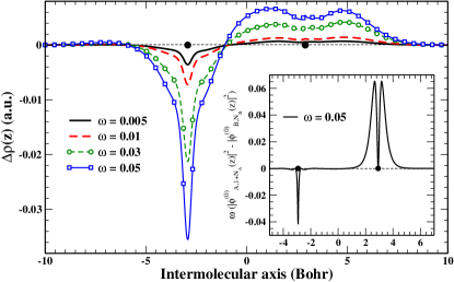
Figure 1: Deviations of plane-averaged errors on embedding densities computed at different fractional particle numbers $\omega$ from the reference one computed at $\omega=0$, for the Ne-Ne complex. The inset shows the frontier orbitals density difference $|\phi_{A,N_{A}+1}^{(0)}|^{2}-|\phi_{B,N_{B}}^{(0)}|^{2}$. The filled circles on the $x$-axis denote the atoms’ positions

Equation (48) provides three important results. First, the error on the embedding density can be expected to vary, at each point of space, almost linearly near $\omega=0$ and roughly follow the spatial shape of $|\phi_{A,N_{A}+1}^{(0)}|^{2}-|\phi_{B,N_{B}}^{(0)}|^{2}$. This fact is shown in Fig. 1, where we report $\Delta\rho_{\omega}^{+}$ for the Ne-Ne complex and compare it to the shape of the frontier orbitals density difference (in the inset). The second result that can be deduced from Eq. (48) is that the difference between the errors on the embedding density computed at two different (small) values of the fractional charge $\omega_{1}$ and $\omega_{2}$ is roughly proportional to $\Delta\omega=\omega_{2}-\omega_{1}$ (see Fig. 2). More precisely we have

$$\Delta\rho_{\omega_{2}}^{+}-\Delta\rho_{\omega_{1}}^{+}=A_{1}^{+}\Delta\omega+A_{2}^{+}(\omega_{2}+\omega_{1})\Delta\omega+\mathcal{O}\left((\omega_{2}+\omega_{1})^{2}\right)\ .$$ (49)

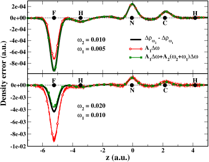
Figure 2: Differences between errors on embedding densities computed using different values of the fractional occupation $\omega$ and comparison with the theoretical formula of Eq. (49). The plot is on an axis parallel to the intermolecular axis of the HF-NCH complex and displaced 0.5 a.u. from the atoms’ plane.

Finally, we see that in order to minimize the error on the embedding density the $\Delta\rho_{0}$ and $\omega A_{1}^{+}$ terms must cancel each other (unless they are both zero, which however brings back to the exact embedding case). This situation is likely to occur if $\Delta\rho_{0}\approx\omega(|\phi_{A,N_{A}+1}^{(0)}|^{2}-|\phi_{B,N_{B}}^{(0)}|^{2})$ (the relaxation term is in general rather small). Thus, the error will be minimized if the error $\Delta\rho_{0}$ is dominated by a (small) charge-transfer of $\omega$ electrons from the subsystem A to the subsystem B. This suggests that the error on the embedding density is minimized by non-zero values of $\omega$ for charge-transfer complexes, whereas it is minimum close to $\omega=0$ for other types of non-covalent complexes (e.g. hydrogen bond, dipole-dipole, or dispersion complexes).

This result finds support in Fig. 3 where we report the integrated error on embedding density

$$\xi_{\omega}=\frac{1000}{N_{A}+N_{B}}\int\left|\Delta\rho_{\omega}^{\pm}(\mathbf{r})\right|d\mathbf{r}$$ (50)

for various non-covalent complexes. Inspection of the plots shows in fact that, as expected, the error is minimized at $\omega=0$ for the Ar-Ne, H₂S-HCl, and HF-NCH complexes, whereas for the charge-transfer complexes Ar-AuF and NH₃-ClF the minimum of $\xi_{\omega}$ is found for $\omega\neq 0$. Note also the quasi linear behavior of the error for different values of $\omega$, in agreement with the previous discussion.

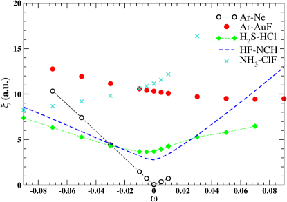
Figure 3: Embedding density errors for all the systems analyzed in this work using different values of the fractional particle number $\omega$.

To conclude this section we add that Eq. (48) can be finally used to obtain some bounds on the absolute error on embedding density, so that

$$\left||\Delta\rho_{0}|\mp\omega|A_{1}^{\pm}|\right|\lessapprox\left|\Delta\rho_{\omega}^{\pm}\right|\lessapprox\left|\Delta\rho_{0}\right|\pm\omega|A_{1}^{\pm}|\ .$$ (51)

III.1 Comments on the embedded Fukui function

The Fukui function Geerlings et al. (2003); Ayers et al. (2009) is an important chemical descriptor defined as the differential change in electron density due to an infinitesimal variation in the particle number. Its meaning is to identify those regions of space where a system is more susceptible of nucleophilic or electrophilic attack, i.e. where it can better accommodate a positive or negative change in the electron number. According to these definitions, in the present case we can define four distinct embedded Fukui functions

$$f^{+}_{A}(\mathbf{r})\equiv\frac{\partial\rho_{A\omega}(\mathbf{r})}{\partial\omega}\Big{|}_{\omega=0^{+}} \ ;\ f^{-}_{B}(\mathbf{r})\equiv-\frac{\partial\rho_{B\omega}(\mathbf{r})}{\partial\omega}\Big{|}_{\omega=0^{+}}$$ (52)

$$f^{-}_{A}(\mathbf{r})\equiv\frac{\partial\rho_{A\omega}(\mathbf{r})}{\partial\omega}\Big{|}_{\omega=0^{-}} \ ;\ f^{+}_{B}(\mathbf{r})\equiv-\frac{\partial\rho_{B\omega}(\mathbf{r})}{\partial\omega}\Big{|}_{\omega=0^{-}}$$ (53)

In fact, Eqs. (52) and (53) imply that large values of $f_{A}^{+}$ in one region of space provide an indication that the embedded subsystem A is able to easily accommodate excess charge in that region, whereas large values of $f_{A}^{-}$ indicate that some charge can be easily removed from a certain region of the embedded subsystem A. Similar considerations hold for subsystem B. We note that the Fukui functions is Eqs. (52) and (53) are defined for $\omega=0^{+}/0^{-}$. This is the most natural definition, because i) in approximated embedding calculations $\omega$=0 gives very often the best results in terms of energy and density (note that the current kinetic-energy functionals fail to describe long-range charge-transfer systems), and ii) it can be directly related to the the case of isolated subsystems.

Moreover, we note that, whenever the subsystem densities are obtained with a full self-consistent procedure, the definitions (52) and (53) present no ambiguity, as the subsystem densities are uniquely defined (using a freeze-and-thaw scheme no arbitrary choice is required for the frozen densities) at any fixed $\omega$. Moreover, because they are obtained within an embedding approach, the resulting Fukui functions fully include all the environmental effects.

The Fukui functions defined in Eqs. (52) and (53) can be further manipulated to obtain important expressions. In order to do this we consider in the following $f_{A}^{+}$; similar derivations can be carried out for all other cases.Using Eq. (38), we can write

$$\frac{\partial\rho_{A\omega}}{\partial\omega} = \rho_{A,N_{A}+1}^{(\omega)}+\omega\frac{\partial\rho_{A,N_{A}+1}^{(\omega)}}{\partial\omega}-$$ (54)

$$-\rho_{A,N_{A}}^{(\omega)}+(1-\omega)\frac{\partial\rho_{A,N_{A}}^{(\omega)}}{\partial\omega}=$$

$$= \left|\phi_{A,N_{A}+1}^{(\omega)}\right|^{2}+\frac{\partial\rho_{A,N_{A}}^{(\omega)}}{\partial\omega}+$$

$$+\omega\left[\frac{\partial\rho_{A,N_{A}+1}^{(\omega)}}{\partial\omega}-\frac{\partial\rho_{A,N_{A}}^{(\omega)}}{\partial\omega}\right]\ .$$

Hence, in the limit $\omega\rightarrow 0^{+}$ we have that the Fukui function is given by the frontier orbital density plus a relaxation term, in agreement with the analogous result obtained via the partition density-functional theory Cohen and Wasserman (2007).

To gain more inside into Eq. (54) we consider however, that the partial derivatives are computed, using the chain rule, as Hellgren and Gross (2012b)

$$\frac{\partial\rho_{A,M}^{(\omega)}(\mathbf{r})}{\partial\omega} = \int\frac{\delta\rho_{A,M}^{(\omega)}(\mathbf{r})}{\delta v^{A}_{s+e}(\mathbf{r}_{1})}\frac{\delta v^{A}_{s+e}(\mathbf{r}_{1})}{\delta\rho_{A\omega}(\mathbf{r}_{2})}\frac{\partial\rho_{A\omega}(\mathbf{r}_{2})}{\partial\omega}d\mathbf{r}_{1}d\mathbf{r}_{2}=$$

$$= \int\chi_{A,M}(\mathbf{r},\mathbf{r}_{1})K_{Hxce}^{A+}(\mathbf{r}_{1},\mathbf{r}_{2})\frac{\partial\rho_{A\omega}(\mathbf{r}_{2})}{\partial\omega}d\mathbf{r}_{1}d\mathbf{r}_{2}\ ,$$

where $v^{A}_{s+e}=v_{s}[\rho_{A\omega}]+v_{emb}^{A}$, $\chi_{A,M}$ is the linear response function of the $M$-particle subsystem A (see Ref. Pavanello, 2013 for details on $\chi_{A,M}$), and $K_{Hxce}^{A+}$ is the Hartree-XC-embedding kernel relative to subsystem A in the case $\omega\geq 0$ (we remark that the XC kernel is discontinuous at integer particle numbers Hellgren and Gross (2012a, b)). We note that in Eq. (LABEL:cbvf) all the derivatives are well defined: in fact, $\rho_{A,M}^{(\omega)}$ is built from $M$ KS orbitals that are all determined by the potential $v^{A}_{s+e}=v_{s}[\rho_{A\omega}]+v_{emb}^{A}$ (see Eq. (19)); on the other hand, $v^{A}_{s+e}$ is clearly a functional of $\rho_{A\omega}$. Then, using Eq. (LABEL:cbvf) into Eq. (54) and taking the limit $\omega\rightarrow 0^{+}$ we finally obtain

$$f_{A}^{+}(\mathbf{r})=\left|\phi_{A,N_{A}+1}^{(0)}(\mathbf{r})\right|^{2}+$$

$$\quad+\int\chi_{A,N_{A}}(\mathbf{r},\mathbf{r}_{1})K_{Hxce}^{A+}(\mathbf{r}_{1},\mathbf{r}_{2})f_{A}^{+}(\mathbf{r}_{2})d\mathbf{r}_{1}d\mathbf{r}_{2}\ .$$ (56)

This expression shows that, in first approximation, the effect of the environment on the Fukui function is simply accounted for by a perturbation induced by the embedding potential on the frontier molecular orbital of the isolated subsystem A. However, the second term includes more subtle effects, since it incorporates not only the response of the subsystem A to the perturbation (the change in the particle number), but also the response of the whole environment to it. In fact, the $K_{Hxce}^{A+}$ kernel contains the functional derivative with respect to $\rho_{A\omega}$ of the embedding potential, which is a bifunctional of both $\rho_{A\omega}$ and $\rho_{B\omega}$ (see Eq. (II.1)). Thus, it contains also contributions proportional to $\delta\rho_{B\omega}/\delta\rho_{A\omega}$, which describe the relaxation of the environment to the nucleophilic attack on the subsystem A.

The fact that the embedded Fukui functions include the effects of the whole system has important consequences. The most important is that (at least for exact embedding) we have an equilibration principle for the embedded Fukui function. In fact, it is easy to show that because $\rho_{A\omega}+\rho_{B\omega}=\rho$ and $\rho$ is independent on $\omega$, we must have at any point in space $f_{A}^{+}=f_{B}^{-}$ (and $f_{A}^{-}=f_{B}^{+}$). The rationale beyond this finding is that the embedding is describing a ground state solution for the whole system. Thus, the propensity to acquire and donate a certain amount of charge must be equal in the whole space to guarantee the stability. This result nicely agrees with that of Eq. (4.28) of Ref. Cohen and Wasserman (2007).

IV Effect of the non-integer particle numbers on the embedding energy

According to Eq. (31) the total energy resulting from the embedding procedure is

$$E^{emb}[\rho_{A\omega},\rho_{B\omega}]=E[\rho_{A\omega}]+E[\rho_{B\omega}]+\mathcal{E}^{nadd}[\rho_{A\omega};\rho_{B\omega}]$$ (57)

with

$$E[\rho_{j}]=T_{s}[\rho_{j}]+\int\rho_{j}(\mathbf{r})v^{j}_{ext}(\mathbf{r})\,d\mathbf{r}+J[\rho_{j}]+E_{xc}[\rho_{j}]$$

(58)

$$\mathcal{E}^{nadd}[\rho_{A\omega};\rho_{B\omega}]=\int\frac{\rho_{A\omega}(\mathbf{r}_{1})\rho_{B\omega}(\mathbf{r}_{2})}{\left|\mathbf{r}_{1}-\mathbf{r}_{2}\right|}d\mathbf{r}_{1}d\mathbf{r}_{2}+$$

$$\ \ \ \ +\int\rho_{B\omega}(\mathbf{r})v^{A}_{ext}(\mathbf{r})d\mathbf{r}+\int\rho_{A\omega}(\mathbf{r})v^{B}_{ext}(\mathbf{r})d\mathbf{r}+$$

$$\ \ \ \ +T_{s}^{nadd}[\rho_{A\omega};\rho_{B\omega}]+E_{xc}^{nadd}[\rho_{A\omega};\rho_{B\omega}]\ ,$$ (59)

where $j=A,B$. For convenience we will call these the subsystems’ and the non-additive contributions to the total energy, respectively. The variation of this energy with respect to $\omega$ can be computed by means of the chain rule $\partial/\partial\omega=\int(\delta/\delta\rho_{j}(\mathbf{r}_{1}))(\partial\rho_{j}(\mathbf{r}_{1})/\partial\omega)d\mathbf{r}_{1}$. Thus, after some algebra (see Appendix A)we obtain

$$\left(\frac{\partial E^{emb}}{\partial\omega}\right)^{\pm}=\mu_{A}^{\pm}-\mu_{B}^{\pm}\ ,$$ (60)

where the $+$ and $-$ superscripts indicate the $\omega>0$ and $\omega<0$ cases, respectively, and $\mu_{A}$ and $\mu_{B}$ are the chemical potentials of the embedded subsystems $A$ and $B$, respectively.

Equation (60) states the simple physical fact that the total embedding energy change upon a transfer of charge $\delta\omega$ from one subsystem to the other is proportional to the difference of the chemical potentials of the two subsystems. This result is analogous to the well known expression for the formation energy in the HSAB theory Chermette (1999).

Of course, for an exact embedding calculation $\mu_{A}^{\pm}=\mu_{B}^{\pm}$ by definition. Thus, the total embedding energy is independent from the fractional charge $\omega$, as it must be. However, for an approximate embedding calculation we can expect the equilibration of the chemical potentials to be incomplete Gritsenko (2013). Then, we can investigate the behavior of the embedding energy error $\Delta E^{emb}_{\omega}=E^{emb}-E_{0}$, where $E_{0}$ is the exact KS total energy of the total system, which is independent on $\omega$. Hence, we can consider

$$\left(\frac{\partial\Delta E^{emb}_{\omega}}{\partial\omega}\right)^{\pm}=\mu_{A}^{\pm}-\mu_{B}^{\pm}\ .$$ (61)

To evaluate the chemical potentials we cannot make direct use of the Janak’s theorem Perdew et al. (1982); Janak (1978), because the energies of the individual interacting subsystems are not well defined in the FDE formalism. Nevertheless, the chemical potentials can be evaluated considering that at each value of $\omega$, despite the energies of the interacting and non-interacting Kohn-Sham systems are different, their chemical potentials are equal by definition. Therefore, focusing, for the moment, on $\mu_{A}^{+}$, we have

$$\mu_{A}^{+}=\left(\frac{\partial E_{s,0}^{A+}}{\partial\omega}\right)_{\rho_{A\omega}}\ ,$$ (62)

where

$$E_{s,0}^{A+}=\mathrm{Tr\left[\hat{H}\hat{\Gamma}_{A}^{KS}\right]}=\omega E_{A,N_{A}+1}^{KS}+(1-\omega)E_{A,N_{A}}^{KS}\ ,$$ (63)

is the energy of the non-interacting embedded Kohn-Sham system (for $\omega>0$), with $\hat{H}$ being the KS Hamiltonian,

$$E_{A,M}^{KS}=\sum_{i}^{M}\epsilon_{A,i}^{(\omega)}\ ,$$ (64)

and $\epsilon_{A,i}^{(\omega)}$ being the eigenvalues of the KSCED for subsystem A. The subscript $\rho_{A\omega}$ recalls that the derivative must be evaluated keeping $\rho_{A\omega}$ fixed, because the equivalence of the Kohn-Sham and the interacting systems only holds at the ground state density (note that this requirement is equivalent to the constraint of fixing the external nuclear potential used in conventional calculations of the chemical potential). However, the embedding potential, depending also on $\rho_{B\omega}$, is allowed to vary.

From Eqs. (62), (63), and (64) we readily find

$$\mu_{A}^{+}=\epsilon_{A,N_{A}+1}^{(\omega)}+\sum_{i}^{N_{A}+1}f_{i}\left(\frac{\partial\epsilon_{A,i}^{(\omega)}}{\partial\omega}\right)_{\rho_{A\omega}}\approx\epsilon_{A,N_{A}+1}^{(\omega)}\ ,$$ (65)

where $f_{i}$ are the occupation numbers. The term depending on the derivatives of the orbital energies is a relaxation term, expressing the response of the system to changes in the embedding potential due to $\omega$-induced variations of $\rho_{B\omega}$. In fact, we can write

$$\left(\frac{\partial\epsilon_{A,i}^{(\omega)}}{\partial\omega}\right)_{\rho_{A\omega}}=\int\frac{\delta\epsilon_{A,i}^{(\omega)}}{\delta v_{emb}^{A}(\mathbf{r}_{1})}\frac{\delta v_{emb}^{A}(\mathbf{r}_{1})}{\delta\rho_{B\omega}(\mathbf{r}_{2})}\frac{\partial\rho_{B\omega}(\mathbf{r}_{2})}{\partial\omega}d\mathbf{r}_{1}d\mathbf{r}_{2}\ .$$ (66)

This term is generally small with respect to the frontier orbital energy and was neglected in the last equality of Eq. (65).

Then, summarizing we find

$$\left(\frac{\partial\Delta E^{emb}_{\omega}}{\partial\omega}\right)^{+} \approx \epsilon_{A,N_{A}+1}^{(\omega)}-\epsilon_{B,N_{B}}^{(\omega)}$$ (67)

$$\left(\frac{\partial\Delta E^{emb}_{\omega}}{\partial\omega}\right)^{-} \approx \epsilon_{A,N_{A}}^{(\omega)}-\epsilon_{B,N_{B}+1}^{(\omega)}\ .$$ (68)

These equations formalize the intuitive idea that, apart for relaxation contributions, the energy change due to the transfer of a fraction of electron from one subsystem to the other is proportional to the difference of the frontier (i.e. with fractional occupation) orbitals eigenvalues.

Equations (67) and (68) are used in Fig. 4 to plot the theoretical behavior (red dashed-lines) of $\partial\Delta E^{emb}_{\omega}/\partial\omega$ for several non-covalent complexes and compare it to numerical results (black dots) from embedding calculations at different $\omega$. Fig. 4 shows that very large errors (10-50 mHa) are present in the energy already for very small $\omega$ values. (at $\omega=0$ the errors are 0.14, -9.07 and 0.43 mHa, for Ne-Ne, NaCl and HF-NCH, respectively). This behavior is related to the incorrect kinetic energy potential which largely fails to reproduce the total density (see e.g. Fig. 2 for the Ne dimer) and the chemical potentials of embedded subsystems. The observed strong asymmetry for positive and negative $\omega$ values in the plot of Na-Cl (partitioned as Na⁺ and Cl^-) is related to the asymmetric energy levels of the embedded subsystems. In particular, when $\omega>0$ we add electrons to the LUMO of Na⁺ (at about -2 eV) and we remove electrons from the HOMO of Cl^- (at about -5 eV); on the other hand, when $\omega<0$ we remove electrons from the HOMO of Na⁺ (at about -29 eV) and add electrons to the LUMO of Cl^- (at about -2 eV). Thus, only for $\omega>0$ the chemical potentials (i.e. the fractional occupied orbitals) are almost aligned, which corresponds to lower slopes through Eqs. (60) and (61).

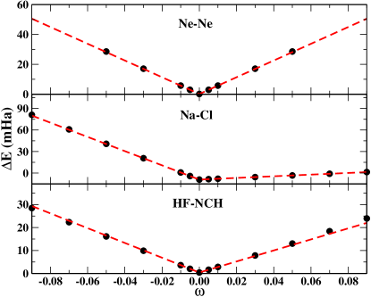
Figure 4: Embedding energy errors $\Delta E_{\omega}^{emb}$ (filled circles) at different values of the fractional occupation $\omega$. Dashed lines indicate theoretical fits according to Eqs. (67) and (68). In all calculations we used revAPBEk functional for the non-additive kinetic energy and a supermolecular def2-TZVPPD basis set. All values reported in these plots are in mHa.

We acknowledge that similar plots for the behavior of the total energy as a function of the subsystems’ occupations were also reported within PDFT Tang et al. (2012). In both cases the cusp originates from the inability of the embedding/partition potential to correctly align the subsystems’ chemical potentials (i.e. the orbitals with fractional occupation). However, the reasons for this drawback are different in the two cases because of the basic theoretical differences between the two methods. In fact, in our FDE treatment the embedding potential is incorrect (for every occupation number) due to the approximations in the kinetic energy functional, while in Ref. Tang et al., 2012 the embedding potential is exact (by construction) only for the “true” occupation numbers.

IV.1 Comments on the derivative discontinuity

Equations (67) and (68) establish a relation between the variation of the embedding total energy (or equivalently of the error on the embedding energy) with the fractional charge and the difference in the frontier orbital energies of the two subsystems. However, for an exact embedding calculation the embedding energy must be independent from the fractional charge. Thus, we must have

$$\epsilon_{A,N_{A}+1}^{(\omega)}\approx\epsilon_{B,N_{B}}^{(\omega)} \mathrm{for}\ \ \omega>0$$ (69)

$$\epsilon_{A,N_{A}}^{(\omega)}\approx\epsilon_{B,N_{B}+1}^{(\omega)} \mathrm{for}\ \ \omega<0\ .$$ (70)

These equations are rationalized in terms of the need for the two subsystems to align their frontier orbital levels in order to achieve electrochemical equilibrium. This behavior is independent on the amount of charge transferred, provided that $\omega\neq 0$. On the other hand, no such need arises when $\omega=0$. In fact, in this case we rather would have

$$\frac{\epsilon_{A,N_{A}+1}^{(0)}+\epsilon_{A,N_{A}}^{(0)}}{2}\approx\frac{\epsilon_{B,N_{B}+1}^{(0)}+\epsilon_{B,N_{B}}^{(0)}}{2}\ .$$ (71)

Thus, a clear discontinuity can be observed in the system when the fractional charge is turned on.

This discontinuous behavior is triggered by a discontinuity in the embedding potential at integer subsystems’ occupations. The effect of a discontinuity in the potential is in fact to promote a sudden shift in the orbital energies. On the other hand, the effect cannot be ascribed to the discontinuity in the Kohn-Sham potential and related kinetic energy, because these already act on the isolated subsystems. Thus, the whole shift required for equilibration must be related to a derivative discontinuity of the non-additive embedding contributions.

Using Eq. (59) indeed we find

$$v_{emb}^{A\pm} = \left(\frac{\delta\mathcal{E}^{nadd}}{\delta\rho_{A\omega}}\right)^{\pm}=\frac{\delta T_{s}[\rho_{A\omega}+\rho_{B\omega}]}{\delta(\rho_{A\omega}+\rho_{B\omega})}-$$ (72)

$$-\left(\frac{\delta T_{s}[\rho_{A\omega}]}{\delta\rho_{A\omega}}\right)^{\pm}+\left(\frac{\delta E_{xc}[\rho_{A\omega}+\rho_{B\omega}]}{\delta(\rho_{A\omega}+\rho_{B\omega})}\right)^{\pm}-$$

$$-\left(\frac{\delta E_{xc}[\rho_{A\omega}]}{\delta\rho_{A\omega}}\right)^{\pm}+v_{J}^{B}+v_{ext}^{B}$$

$$v_{emb}^{B\pm} = \left(\frac{\delta\mathcal{E}^{nadd}}{\delta\rho_{B\omega}}\right)^{\pm}=\frac{\delta T_{s}[\rho_{A\omega}+\rho_{B\omega}]}{\delta(\rho_{A\omega}+\rho_{B\omega})}-$$ (73)

$$-\left(\frac{\delta T_{s}[\rho_{B\omega}]}{\delta\rho_{B\omega}}\right)^{\pm}+\left(\frac{\delta E_{xc}[\rho_{A\omega}+\rho_{B\omega}]}{\delta(\rho_{A\omega}+\rho_{B\omega})}\right)^{\pm}-$$

$$-\left(\frac{\delta E_{xc}[\rho_{B\omega}]}{\delta\rho_{B\omega}}\right)^{\pm}+v_{J}^{A}+v_{ext}^{A}\ ,$$

where we used the fact that $\delta(\rho_{A\omega}(\mathbf{r}_{1})+\rho_{B\omega}(\mathbf{r}_{1}))/\delta\rho_{i}(\mathbf{r}_{2})=\delta(\mathbf{r}_{1}-\mathbf{r}_{2})$. Note that the $\pm$ superscript was used neither for $\delta T_{s}[\rho_{A\omega}+\rho_{B\omega}]/\delta(\rho_{A\omega}+\rho_{B\omega})$, since this derivative is computed for the integer density $\rho_{A\omega}+\rho_{B\omega}$, nor for $v_{J}$ and $v_{ext}$ that are continuous functionals of the density. As a consequence, the discontinuity of the embedding potential is found to be

$$\Delta_{emb}^{A} \equiv v_{emb}^{A+}-v_{emb}^{A-}=\left(\frac{\delta T_{s}[\rho_{A\omega}]}{\delta\rho_{A\omega}}\right)^{-}-\left(\frac{\delta T_{s}[\rho_{A\omega}]}{\delta\rho_{A\omega}}\right)^{+}+$$ (74)

$$+\left(\frac{\delta E_{xc}[\rho_{A\omega}]}{\delta\rho_{A\omega}}\right)^{-}-\left(\frac{\delta E_{xc}[\rho_{A\omega}]}{\delta\rho_{A\omega}}\right)^{+}$$

$$\Delta_{emb}^{B} \equiv v_{emb}^{B+}-v_{emb}^{B-}=\left(\frac{\delta T_{s}[\rho_{B\omega}]}{\delta\rho_{B\omega}}\right)^{-}-\left(\frac{\delta T_{s}[\rho_{B\omega}]}{\delta\rho_{B\omega}}\right)^{+}+$$ (75)

$$+\left(\frac{\delta E_{xc}[\rho_{B\omega}]}{\delta\rho_{B\omega}}\right)^{-}-\left(\frac{\delta E_{xc}[\rho_{B\omega}]}{\delta\rho_{B\omega}}\right)^{+}\ .$$

These discontinuities are exactly opposite to those due to the KS potential and the non-interacting kinetic energy in each (isolated) subsystem

$$\Delta_{s}^{A} = \left(\frac{\delta T_{s}[\rho_{A\omega}]}{\delta\rho_{A\omega}}\right)^{+}-\left(\frac{\delta T_{s}[\rho_{A\omega}]}{\delta\rho_{A\omega}}\right)^{-}+$$ (76)

$$+\left(\frac{\delta E_{xc}[\rho_{A\omega}]}{\delta\rho_{A\omega}}\right)^{+}-\left(\frac{\delta E_{xc}[\rho_{A\omega}]}{\delta\rho_{A\omega}}\right)^{-}$$

$$\Delta_{s}^{B} = \left(\frac{\delta T_{s}[\rho_{B\omega}]}{\delta\rho_{B\omega}}\right)^{+}-\left(\frac{\delta T_{s}[\rho_{B\omega}]}{\delta\rho_{B\omega}}\right)^{-}+$$ (77)

$$+\left(\frac{\delta E_{xc}[\rho_{B\omega}]}{\delta\rho_{B\omega}}\right)^{+}-\left(\frac{\delta E_{xc}[\rho_{B\omega}]}{\delta\rho_{B\omega}}\right)^{-}\ .$$

Thus, two main cases can be considered. (1) Both the exchange-correlation and the kinetic energy are treated in the same way (eventually exactly) in the subsystems’ and the non-additive contributions to the total energy. This corresponds to an exact embedding treatment. In this case the discontinuities cancel each other and the derivative of the total embedding energy is continuous at integer subsystems’ particle numbers. In fact, the embedding energy is even constant, because the discontinuity in the embedding potential is such as to force the equilibration of the subsystems’ chemical potentials at any $\omega$. (2) The exchange-correlation energy is treated in the same way both in the subsystems’ and the non-additive contributions to the total energy but the kinetic energy is not. Typically, in a KS framework we would have that the non-interacting kinetic energy is exact in the subsystems’ contributions to the total energy but approximate by a semilocal functional in the non-additive one. This is the usual case in practical embedding calculations. In this situation the total exchange-correlation discontinuity in $\Delta_{emb}^{i}+\Delta_{s}^{i}$ cancels out, however there is no discontinuity in the embedding kinetic term of $\Delta_{emb}^{i}$ because a semilocal kinetic approximation is used. Thus, the KSCED equations include a spurious kinetic derivative discontinuity. As a result the derivative of the total embedding energy displays a cusp at integer subsystems’ particle numbers. This cusp is determined by the kinetic derivative discontinuity and therefore is equal to the frontier orbitals eigenvalues difference Yang et al. (2012); Sagvolden and Perdew (2008) , in agreement with Eqs. (67) and (68).

IV.2 Comments on the embedded chemical hardness

The global hardness is defined as the derivative of the chemical potential with respect to the particles number at fixed nuclear environment Parr and Yang (1989); Chattaraj (2009); Chermette (1999); Geerlings et al. (2003). Because the nuclear potential is piecewise constant, at zero temperature this definition is not well posed, since the forward and backward derivatives are always zero while the central derivative diverges. Thus, in practice, at zero temperature, the original definition of the hardness is replaced by the difference of the chemical potentials computed at $N+\delta$ and $N-\delta$, respectively, with $\delta\rightarrow 0^{+}$.

Thus, we can define the embedded subsystems’ hardnesses as

$$\eta_{A}\equiv\mu_{A}^{+}-\mu_{A}^{-}\quad;\quad\eta_{B}\equiv-(\mu_{B}^{+}-\mu_{B}^{-})\ .$$ (78)

These definitions respect the general features associated to the concept of chemical hardness Parr and Yang (1989). In particular, the fact that a small hardness corresponds to the possibility to easy add or remove charge from the (embedded) system, whereas a high hardness implies the opposite. Equations (78) include into the hardness of each subsystem the environmental effects (due to the other subsystem), thus they provide an indicator for the possibility that a component of a complex may interact with a third system (e.g., we can obtain the hardness of an acidic complex when solvated and compare it to that of a basic complex immersed in the same solution).

Using Eq. (65), the embedded hardness can be easily calculated to be

$$\eta_{A} = \epsilon_{A,N_{A}+1}^{(0)}-\epsilon_{A,N_{A}}^{(0)}+$$

$$+\sum_{i}^{N_{A}+1}\left(\frac{\partial\epsilon_{A,i}^{(0)}}{\partial\omega}\right)_{\rho_{A\omega}}^{+}-\sum_{i}^{N_{A}}\left(\frac{\partial\epsilon_{A,i}^{(0)}}{\partial\omega}\right)_{\rho_{A\omega}}^{-}$$

$$\eta_{B} = \epsilon_{B,N_{B}+1}^{(0)}-\epsilon_{B,N_{B}}^{(0)}+$$

$$+\sum_{i}^{N_{B}+1}\left(\frac{\partial\epsilon_{B,i}^{(0)}}{\partial\omega}\right)_{\rho_{B\omega}}^{+}-\sum_{i}^{N_{B}}\left(\frac{\partial\epsilon_{B,i}^{(0)}}{\partial\omega}\right)_{\rho_{B\omega}}^{-}\ ,$$

where we took the limits $\omega\rightarrow 0^{+}$ and $\omega\rightarrow 0^{-}$ as appropriate. As we observed for the chemical potential the relaxation terms are usually small. Moreover, the two relaxation contributions tend to cancel each other, apart for differences originating in the discontinuities of the embedding potential derivative. Thus, it may be appropriate in most situations to consider the approximate expressions

$$\eta_{A}\approx\epsilon_{A,N_{A}+1}^{(0)}-\epsilon_{A,N_{A}}^{(0)}\quad;\quad\eta_{B}\approx\epsilon_{B,N_{B}+1}^{(0)}-\epsilon_{B,N_{B}}^{(0)}\ .$$ (81)

V Computational details

To test some of the results of theoretical analysis of the previous sections FDE calculations were performed on a set of representative non-covalent complexes (Ne-Ne, Ne-Ar, Ar-AuF, H₂S-HCl, HF-NCH, (NH₃)₂, NH₃-ClF and NaCl). Note that NaCl is partitioned as Na⁺/Cl^-. The structures of the complexes were taken from Refs. Zhao and Truhlar, 2005a, b; Beyhan et al., 2010; Wesolowski et al., 1996.

The test set was restricted to contain only non-covalently bound systems because these are the only ones that can be properly described in FDE calculations at the current state of the art. On the other hand, strongly interacting complexes, despite being potentially interesting systems to be studied with FDE calculations using fractional subsystems’ occupations, were not considered in the present work to keep the analysis and the discussion more clear.

All calculations were performed with a development version of the FDE script Laricchia et al. (2010), interfaced with the TURBOMOLE program package TUR , version 6.4. In all cases a freeze-and-thaw procedure Wesolowski and Weber (1996) was used to guarantee the full relaxation of the embedded ground-state electron density of both subsystems, until dipole moments of the embedded subsystems converged to $10^{-3}$ au. A supermolecular def2-TZVPPD Weigend et al. (2003); Weigend and Ahlrichs (2005) basis set was employed in all calculations to expand the subsystem electron densities. The def2-TZVPPD basis set adds diffuse basis functions to the def2-TZVPP Weigend and Ahlrichs (2005) basis set, thus granting an accurate representation for the electron densities even at the relatively large bonding distances characteristic of the systems under consideration. Very accurate integration grids were employed to minimize numerical errors. Additional details about our implementation and computational procedure are reported in Refs. Laricchia et al., 2010, 2012. The calculations were performed using the semilocal PBE XC functional Perdew et al. (1996), while the revAPBEk Laricchia et al. (2011b); Constantin et al. (2011); apbekroutine functional was used to approximate the non-additive non-interacting kinetic energy term.

VI Conclusions

In this paper we extended the FDE theory to the treatment of non-integer subsystems’ particle numbers and discussed the relevance of this extension for the outcome of practical frozen-density simulations. In particular, we were able to show that, in approximate FDE applications, the resulting densities and total energies have a well defined behavior as functions of the fractional occupations of the subsystems. We remark that this is a unique feature of the FDE theory, whereas no such a dependence can be exploited in PDFT and potential-functional embedding theory Huang and Carter (2011) because in these cases the occupation numbers are not defined a priori within the partitioning scheme but are instead determined variationally.

Examining the variation of the total embedding energy with the subsystems’ particle numbers we could provide an explicit expression for the discontinuity of the embedding potential at integer particles numbers. Thus, it was possible to highlight the relevance of the kinetic derivative discontinuity in determining the behavior of the embedding potential, which becomes evident as a cusp at integer particle numbers for any approximate frozen-density embedding calculation.

Moreover, taking advantage of our definitions of densities and chemical potentials at different subsystems’ particle numbers, we could introduce a rigorous definition of some important chemical descriptors within the FDE theory, in agreement with previous work done in the context of PDFTCohen and Wasserman (2007). Thus, despite a full discussion of chemical reactivity theory was well beyond the scope of this paper, we were able to indicate some important properties of the Fukui function and the global hardness in relation to the embedding environment.

Finally, we remark that the present work constitutes an important ground on which several future developments may be built. In particular, we mention (1) the possibility to extend the present theory to the case of a generalized KS formalism, so that also hybrid functionals can be considered; (2) the consideration of total systems with ensemble densities; and (3) the full investigation of the dependence of chemical reactivity indexes on the environment.

Appendix A Proof of Eq. (60)

In this appendix we provide a sketch of the proof of Eq. (60).

Starting from Eqs. (57), (58), and (59) and using the chain rule for derivation we can write, after a bit of algebra,

$$\left(\frac{\partial E^{emb}}{\partial\omega}\right)^{\pm}=$$

$$=\int\left(\frac{\delta T_{s}[\rho_{A\omega}]}{\delta\rho_{A\omega}(\mathbf{r}_{1})}+v_{s}[\rho_{A\omega}](\mathbf{r}_{1})+v_{emb}^{A}(\mathbf{r}_{1})\right)\left(\frac{\partial\rho_{A\omega}(\mathbf{r}_{1})}{\partial\omega}\right)^{\pm}d\mathbf{r}_{1}+$$

$$+\int\left(\frac{\delta T_{s}[\rho_{B\omega}]}{\delta\rho_{B\omega}(\mathbf{r}_{1})}+v_{s}[\rho_{B\omega}](\mathbf{r}_{1})+v_{emb}^{B}(\mathbf{r}_{1})\right)\left(\frac{\partial\rho_{B\omega}(\mathbf{r}_{1})}{\partial\omega}\right)^{\pm}d\mathbf{r}_{1}\ ,$$

where a $+$ in the superscript indicates that we are dealing with $\omega>0$, whereas a $-$ denotes that we are considering $\omega<0$. Because $\rho_{A\omega}$ and $\rho_{B\omega}$ are solutions of the Euler equations defined by the first term in parenthesis inside each integral, we can substitute these by the respective chemical potentials (see Eqs. (17) and (18)). Hence,

$$\left(\frac{\partial E^{emb}}{\partial\omega}\right)^{\pm}=\mu_{A}^{\pm}\int\left(\frac{\partial\rho_{A\omega}(\mathbf{r}_{1})}{\partial\omega}\right)^{\pm}+\mu_{B}^{\pm}\int\left(\frac{\partial\rho_{B\omega}(\mathbf{r}_{1})}{\partial\omega}\right)^{\pm}\ .$$ (82)

To complete the proof we note that

$$\int\left(\frac{\partial\rho_{A\omega}(\mathbf{r}_{1})}{\partial\omega}\right)^{\pm}d\mathbf{r}_{1} = \frac{\partial}{\partial\omega}\left(\int\rho_{A\omega}(\mathbf{r}_{1})d\mathbf{r}_{1}\right)^{\pm}=$$ (83)

$$= \frac{\partial(N_{A}+\omega)}{\partial\omega}=1$$

$$\int\left(\frac{\partial\rho_{B\omega}(\mathbf{r}_{1})}{\partial\omega}\right)^{\pm}d\mathbf{r}_{1} = \frac{\partial}{\partial\omega}\left(\int\rho_{B\omega}(\mathbf{r}_{1})d\mathbf{r}_{1}\right)^{\pm}=$$ (84)

$$= \frac{\partial(N_{B}-\omega)}{\partial\omega}=-1\ .$$

Therefore, we finally find

$$\left(\frac{\partial E^{emb}}{\partial\omega}\right)^{\pm}=\mu_{A}^{\pm}-\mu_{B}^{\pm}\ .$$ (85)

Acknowledgments:

This work was partially funded by the ERC Starting Grant FP7 Project DEDOM (No. 207441). We thank TURBOMOLE GmbH for providing the TURBOMOLE program package and M. Margarito for technical support.

References

- Senatore and Subbaswamy (1986) G. Senatore and K. R. Subbaswamy, Phys. Rev. B 34, 5754 (1986).
- Cortona (1991) P. Cortona, Phys. Rev. B 44, 8454 (1991).
- Yang (1991) W. Yang, Phys. Rev. Lett. 66, 1438 (1991).
- Cortona and Monteleone (1994) P. Cortona and A. V. Monteleone, Int. J. Quantum Chem. 52, 987 (1994).
- Yang and Lee (1995) W. Yang and T.-S. Lee, J. Chem. Phys. 103, 5674 (1995).
- ichirou Sugiki et al. (2003) S. Sugiki, N. Kurita, Y. Sengoku, and H. Sekino, Chem. Phys. Lett. 382, 611 (2003).
- Fedorov and Kitaura (2004) D. G. Fedorov and K. Kitaura, Chem. Phys. Lett. 389, 129 (2004).
- Huang and Carter (2006) P. Huang and E. A. Carter, J. Chem. Phys. 125, 084102 (2006).
- Wesolowski (2006) T. A. Wesolowski, in Computational Chemistry: Reviews of Current Trends, edited by J. Leszczynski (World Scientific, Singapore, 2006), vol. 10 of Computational Chemistry: Reviews of Current Trends, chap. 1, pp. 1–82.
- Cohen and Wasserman (2007) M. H. Cohen and A. Wasserman, J. Phys. Chem. A 111, 2229 (2007).
- Cohen et al. (2007) M. H. Cohen, A. Wasserman, and K. Burke, J. Phys. Chem. A 111, 12447 (2007).
- Akama et al. (2007) T. Akama, M. Kobayashi, and H. Nakai, J. Comput. Chem. 28, 2003 (2007).
- Wang et al. (2008) L.-W. Wang, Z. Zhao, and J. Meza, Phys. Rev. B 77, 165113 (2008).
- Zhao et al. (2008) Z. Zhao, J. Meza, and L.-W. Wang, J. Phys.: Condensed Matter 20, 294203 (2008).
- He et al. (2009) J. He, C. D. Paola, and L. Kantorovich, J. Chem. Phys. 130, 144104 (pages 18) (2009).
- Elliott et al. (2010) P. Elliott, K. Burke, M. H. Cohen, and A. Wasserman, Phys. Rev. A 82, 024501 (2010).
- Huang and Carter (2011) C. Huang and E. A. Carter, J. Chem. Phys. 135, 194104 (pages 17) (2011).
- (18) C. Huang, M. Pavone, and E. A. Carter, J. Chem. Phys. 134, 154110 (2011).
- Gordon et al. (2012) M. S. Gordon, D. G. Fedorov, S. R. Pruitt, and L. V. Slipchenko, Chem. Rev. 112, 632 (2012).
- Severo Pereira Gomes and Jacob (2012) A. Severo Pereira Gomes and C. R. Jacob, Annu. Rep. Prog. Chem., Sect. C: Phys. Chem. 108, 222 (2012).
- Manby et al. (2012) F. R. Manby, M. Stella, J. D. Goodpaster, and T. F. Miller, J. Chem. Theory Comput. 8, 2564 (2012).
- Wesolowski and Wang (2013) T. A. Wesolowski and Y. A. Wang, eds., Recent Progress in Orbital-free Density Functional Theory, vol. 6 of Recent Advances in Computational Chemistry (World Scientific, Singapore, 2013).
- Hohenberg and Kohn (1964) P. Hohenberg and W. Kohn, Phys. Rev. 136, B864 (1964).
- Parr and Yang (1989) R. G. Parr and W. Yang, eds., Density Functional Theory of Atoms and Molecules (Oxford Univeristy Press, New York, 1989).
- Wesolowski and Warshel (1993) T. A. Wesolowski and A. Warshel, J. Phys. Chem. 97, 8050 (1993).
- Neugebauer et al. (2005a) J. Neugebauer, C. R. Jacob, T. A. Wesolowski, and E. J. Baerends, J. Phys. Chem. A 109, 7805 (2005a).
- Jacob et al. (2006) C. R. Jacob, J. Neugebauer, L. Jensen, and L. Visscher, Phys. Chem. Chem. Phys. 8, 2349 (2006).
- Jacob et al. (2008) C. R. Jacob, J. Neugebauer, and L. Visscher, J. Comput. Chem. 29, 1011 (2008).
- Wesołowski (2008) T. A. Wesołowski, Phys. Rev. A 77, 012504 (2008).
- Neugebauer (2009a) J. Neugebauer, J. Chem. Phys. 131, 084104 (2009a).
- Laricchia et al. (2010) S. Laricchia, E. Fabiano, and F. Della Sala, J. Chem. Phys. 133, 164111 (2010).
- Kaminski et al. (2010) J. W. Kaminski, S. Gusarov, T. A. Wesolowski, and A. Kovalenko, J. Phys. Chem. A 114, 6082 (2010).
- Fux et al. (2010) S. Fux, C. R. Jacob, J. Neugebauer, L. Visscher, and M. Reiher, J. Chem. Phys. 132, 164101 (2010).
- owski (2011) T. A. Wesolowski, J. Chem. Phys. 135, 027101 (pages 2) (2011).
- Fux et al. (2011) S. Fux, C. R. Jacob, J. Neugebauer, L. Visscher, and M. Reiher, J. Chem. Phys. 135, 027102 (2011).
- Pavanello and Neugebauer (2011) M. Pavanello and J. Neugebauer, J. Chem. Phys. 135, 234103 (2011).
- Laricchia et al. (2011a) S. Laricchia, E. Fabiano, and F. Della Sala, Chem. Phys. Lett. 518, 114 (2011a).
- Aquilante and owski (2011) F. Aquilante and T. A. Wesolowski, J. Chem. Phys. 135, 084120 (2011).
- de Silva and Wesolowski (2012) P. de Silva and T. A. Wesolowski, J. Chem. Phys. 137, 094110 (2012).
- Laricchia et al. (2012) S. Laricchia, E. Fabiano, and F. Della Sala, J. Chem. Phys. 137, 014102 (2012).
- (41) C. R. Jacob and J. Neugebauer, WIREs Comput Mol Sci. (2014), doi: 10.1002/wcms.1175.
- Neugebauer et al. (2005b) J. Neugebauer, M. J. Louwerse, E. J. Baerends, and T. A. Wesolowski, J. Chem. Phys. 122, 094115 (2005b).
- Jacob et al. (2005) C. R. Jacob, T. A. Wesolowski, and L. Visscher, J. Chem. Phys. 123, 174104 (2005).
- Kevorkyants et al. (2006) R. Kevorkyants, M. Dulak, and T. A. Wesolowski, J. Chem. Phys. 124, 024104 (2006).
- Dulak and Wesolowski (2007) M. Dulak and T. Wesolowski, J. Mol. Model. 13, 631 (2007).
- Dulak et al. (2007) M. Dulak, J. W. Kamiński, and T. A. Wesolowski, J. Chem. Theory Comput. 3, 735 (2007).
- Neugebauer (2009b) J. Neugebauer, ChemPhysChem 10, 3148 (2009b).
- Götz et al. (2009) A. W. Götz, S. M. Beyhan, and L. Visscher, J. Chem. Theory Comput. 5, 3161 (2009).
- Constantin et al. (2011) L. A. Constantin, E. Fabiano, S. Laricchia, and F. Della Sala, Phys. Rev. Lett. 106, 186406 (2011).
- Laricchia et al. (2011b) S. Laricchia, E. Fabiano, L. A. Constantin, and F. Della Sala, J. Chem. Theory Comput. 7, 2439 (2011b).
- Fradelos and Wesołowski (2011) G. Fradelos and T. A. Wesolowski, J. Phys. Chem. A 115, 10018 (2011).
- Fradelos et al. (2011) G. Fradelos, J. J. Lutz, T. A. Wesolowski, P. Piecuch, and M. Włoch, J. Chem. Theory Comput. 7, 1647 (2011).
- Laricchia et al. (2013) S. Laricchia, E. Fabiano, and F. Della Sala, J. Chem. Phys. 138, 124112 (2013).
- Kohn and Sham (1965) W. Kohn and L. J. Sham, Phys. Rev. 140, A1133 (1965).
- Elliott et al. (2009) P. Elliott, M. H. Cohen, A. Wasserman, and K. Burke, J. Chem. Theory Comput. 5, 827 (2009).
- Tang et al. (2012) R. Tang, J. Nafziger, and A. Wasserman, Phys. Chem. Chem. Phys. 14, 7780 (2012).
- (57) M A. Mosquera and A. Wasserman, Mol. Phys. 111, 505 (2013).
- Perdew et al. (1982) J. P. Perdew, R. G. Parr, M. Levy, and J. L. Balduz, Phys. Rev. Lett. 49, 1691 (1982).
- Janak (1978) J. F. Janak, Phys. Rev. B 18, 7165 (1978).
- Yang et al. (2012) W. Yang, A. J. Cohen, and P. Mori-Sánchez, J. Chem. Phys. 136, 204111 (2012).
- Cohen et al. (2012) A. J. Cohen, P. Mori-Sánchez, and W. Yang, Chemical Reviews 112, 289 (2012).
- Cohen et al. (2008a) A. J. Cohen, P. Mori-Sánchez, and W. Yang, Science 321, 792 (2008a).
- Cohen et al. (2008b) A. J. Cohen, P. Mori-Sánchez, and W. Yang, Phys. Rev. B 77, 115123 (2008b).
- Fabiano and Constantin (2013) E. Fabiano and L. A. Constantin, Phys. Rev. A 87, 012511 (2013).
- Chattaraj (2009) P. K. Chattaraj, ed., Chemical Reactivity Theory: A Density Functional View (CRC Press, Boca Raton, FL, USA, 2009).
- Chermette (1999) H. Chermette, J. Comput. Chem. 20, 129 (1999).
- Geerlings et al. (2003) P. Geerlings, F. De Proft, and W. Langenaeker, Chem. Rev. 103, 1793 (2003).
- Levy (1979) M. Levy, Proc. Natl. Acad. Sci. 76, 6062 (1979).
- Lieb (1983) E. H. Lieb, Int. J. Quant. Chem. 24, 243 (1983).
- Scuseria and Staroverov (2005) G. E. Scuseria and V. N. Staroverov, in Theory and Applications of Computational Chemistry: The First 40 Years (A Volume of Technical and Historical Perspectives), edited by C. E. Dykstra, G. Frenking, K. S. Kim, and G. E. Scuseria (Elsevier, Amsterdam, 2005), chap. 24, p. 669–724.
- Wesolowski and Weber (1997) T. A. Wesolowski and J. Weber, Int. J. Quant. Chem. 61, 303 (1997).
- Ullrich and Kohn (2001) C. A. Ullrich and W. Kohn, Phys. Rev. Lett. 87, 093001 (2001).
- Kraisler and Kronik (2013) E. Kraisler and L. Kronik, Phys. Rev. Lett. 110, 126403 (2013).
- Kiewisch et al. (2008) K. Kiewisch, G. Eickerling, M. Reiher, and J. Neugebauer, J. Chem. Phys. 128, 044114 (2008).
- Wesolowski and Weber (1996) T. A. Wesolowski and J. Weber, Chem. Phys. Lett. 248, 71 (1996).
- Fabiano et al. (2011) E. Fabiano, L. A. Constantin, and F. Della Sala, J. Chem. Theory Comput. 7, 3548 (2011).
- Goerigk and Grimme (2010) L. Goerigk and S. Grimme, J. Chem. Theory Comput. 6, 107 (2010).
- Gritsenko (2013) O. V. Gritsenko, in Recent Progress in Orbital-free Density Functional Theory, edited by T. A. Wesolowski and Y. A. Wang (World Scientific, Singapore, 2013), vol. 6 of Recent Advances in Computational Chemistry, chap. 12, pp. 355–365.
- Ayers et al. (2009) P. W. Ayers, W. Yang, and L. J. Bartolotti, in Chemical Reactivity Theory: A Density Functional View, edited by P. K. Chattaraj (CRC Press, Boca Raton, FL, USA, 2009), chap. 18, pp. 255–267.
- Pavanello (2013) M. Pavanello, J. Chem. Phys. 138, 204118 (2013).
- Hellgren and Gross (2012a) M. Hellgren and E. K. U. Gross, Phys. Rev. A 85, 022514 (2012a).
- Hellgren and Gross (2012b) M. Hellgren and E. K. U. Gross, J. Chem. Phys. 136, 114102 (2012b).
- Sagvolden and Perdew (2008) E. Sagvolden and J. P. Perdew, Phys. Rev. A 77, 012517 (2008).
- Zhao and Truhlar (2005a) Y. Zhao and D. G. Truhlar, J. Chem. Theory Comput. 1, 415 (2005a).
- Zhao and Truhlar (2005b) Y. Zhao and D. G. Truhlar, J. Phys. Chem. A 109, 5656 (2005b).
- Beyhan et al. (2010) S. M. Beyhan, A. W. Götz, C. R. Jacob, and L. Visscher, J. Chem. Phys. 132, 044114 (2010).
- Wesolowski et al. (1996) T. A. Wesolowski, H. Chermette, and J. Weber, J. Chem. Phys. 105, 9182 (1996).
-
(88)
TURBOMOLE V6.4 2012, a development of University of
Karlsruhe and Forschungszentrum Karlsruhe GmbH, 1989-2007, TURBOMOLE
GmbH, since 2007; available from
http://www.turbomole.com. - Weigend et al. (2003) F. Weigend, F. Furche, and R. Ahlrichs, J. Chem. Phys. 119, 12753 (2003).
- Weigend and Ahlrichs (2005) F. Weigend and R. Ahlrichs, Phys. Chem. Chem. Phys. 7, 3297 (2005).
- Perdew et al. (1996) J. P. Perdew, K. Burke, and M. Ernzerhof, Phys. Rev. Lett. 77, 3865 (1996).
- (92) FORTRAN90 routines are available at http://www.theory-nnl.it/software.php.