Two recursive GMRES-type methods for shifted linear systems with general preconditioning

Abstract

We present two minimum residual methods for solving sequences of shifted linear systems, the right-preconditioned shifted GMRES and shifted Recycled GMRES  algorithms which use a seed projection strategy often employed to solve multiple related problems. These methods are compatible with general preconditioning of all systems, and when restricted to right preconditioning, require no extra applications of the operator or preconditioner. These seed projection methods perform a minimum residual iteration for the base system while improving the approximations for the shifted systems at little additional cost. The iteration continues until the base system approximation is of satisfactory quality. The method is then recursively called for the remaining unconverged systems. We present both methods inside of a general framework which allows these techniques to be extended to the setting of flexible preconditioning and inexact Krylov methods. We present some analysis of such methods and numerical experiments demonstrating the effectiveness of the algorithms we have derived.

1 Introduction

We develop techniques for solving a family (or a sequence of families) of linear systems in which the coefficient matrices differ only by a scalar multiple of the identity. There are many applications which warrant the solution of a family of shifted linear systems, such as those arising in lattice quantum chromodynamics (QCD) (see, e.g., [14]) as well as other applications such as Tikhonov-Phillips regularization, global methods of nonlinear analysis, and Newton trust region methods [5]. The goal is to develop a framework in which minimum residual methods can be applied to shifted systems in a way that:

1. allows us to exploit the relationships between the coefficient matrices

2. is compatible with general (right) preconditioning.

In this paper, we use such a framework to propose two new methods: one which is built on top of the GMRES method [31] for solving a family of shifted systems (cf. (1)) and one which is built on top of a GCRO-type augmented Krylov method [10] which, when paired with a harmonic Ritz vector recycling strategy [25, 26], is an extension of the GCRO-DR method [27] to solve a sequence of shifted system families (cf. (2)). To do this, we use a seed projection strategy, often proposed for use in conjunction with short-term recurrence iterative methods [6, 7, 19, 28].

The rest of this paper is organized as follows. In the next section, we discuss some previous strategies to treat such problems and discuss some of their limitations. In Section 3, we review the minimum residual Krylov subspace method GMRES as well as two GMRES variants, one for shifted linear systems and the other extending GMRES to the augmented Krylov subspace setting, i.e., Recycled GMRES. In Section 4, we present a general framework to perform minimum residual projections of the shifted system residuals with respect to the search space generated for the base system. In Subsection 4.1 we use this framework to derive our shifted GMRES method and in Subsection 4.2 we derive a shifted Recycled GMRES  method. In Section 5, we present some analysis of the expected performance of these methods. In Section 6, we present some numerical results before concluding in Section 7.

2 Background

Consider a family of shifted linear systems, which we parameterize by $\ell$, i.e.,

$$\left(\mathbf{A}+\sigma^{(\ell)}\mathbf{I}\right)\mathbf{x}^{(\ell)}=\mathbf{b}\mbox{\ \ \ for\ \ \ }\ell=1,\ldots,L.$$ (1)

We call the numbers $\left\{\sigma^{(\ell)}\right\}_{\ell=1}^{L}\subset\mathbb{C}$ shifts, $\mathbf{A}$ the base matrix, and $\mathbf{A}+\sigma\mathbf{I}$ a shifted matrix. Systems of the form (1) are called shifted linear systems. Krylov subspace methods have been proposed to simultaneously solve this family of systems, see, e.g., [8, 12, 13, 20, 36]. These methods satisfy requirement (a) but are not compatible with general preconditioning strategies, as they rely on the invariance of the Krylov subspace under constant shift of the coefficient matrix; cf. (7). Specially chosen polynomial preconditioners, however, have been shown to be compatible with such methods; see, e.g., [1, 3, 4, 18, 23, 33, 42].

We can introduce an additional parameter $i$, which indexes a sequence of matrices $\left\{\mathbf{A}_{i}\right\}\subset\mathbb{C}^{n\times n}$, and for each $i$, we solve a family of the form

$$\left(\mathbf{A}_{i}+\sigma_{i}^{(\ell)}\mathbf{I}\right)\mathbf{x}_{i}^{(\ell)}=\mathbf{b}_{i}\mbox{\ \ \ for\ \ \ }\ell=1\ldots L_{i}$$ (2)

We consider the case that the right-hand side varies with respect to $\mathbf{A}_{i}$ but not for each shift. What we propose is indeed applicable in the more general setting, but we do not treat that here. Augmented Krylov subspace methods have been proposed for efficiently solving a sequence of linear systems with a slowly changing coefficient matrix, allowing important spectral information generated while solving $\mathbf{A}_{i}\mathbf{x}_{i}=\mathbf{b}_{i}$ to be used to augment the Krylov subspace generated when solving $\mathbf{A}_{i+1}\mathbf{x}_{i+1}=\mathbf{b}_{i+1}$; see, e.g., [27, 32, 41]. In cases such as a Newton iteration, these matrices are available one at a time, while in a case such as an implicit time-stepping scheme, the matrix may not change at all.

In [40], the authors explored solving a family of shifted systems over an augmented Krylov subspace. Specifically, the goal was to develop a method which solved the family of systems simultaneously, using one augmented subspace to extract all candidate solutions, which also had a fixed storage requirement, independent of the number of shifts $L$. It was shown that in general within the framework of GMRES for shifted systems [13] and subspace recycling [27], such a method, does not exist. In the context of subspace recycling for Hermitian linear systems, in the absence of preconditioning Kilmer and de Sturler proposed a MINRES method in a subspace recycling framework which simultaneously solves multiple non-Hermitian systems, which all differ from a real-symmetric system by a complex multiple of the identity [20], by minimizing the shifted residuals over the augmented Krylov subspace subspace, built using the symmetric Lanczos process. In this paper, we focus exclusively on problems in which the base coefficient matrices $\mathbf{A}_{i}$ are non-Hermitian.

A conclusion one can draw from [40] is that we should consider avoiding methods relying on the invariance of Krylov subspaces under a constant shift of the identity; cf. (7). Relying on this invariance imposes restrictions on our ability to develop an algorithm. Furthermore, relying on this shift invariance means we cannot use arbitrary preconditioners. General preconditioners are unavailable if we want to exploit shift invariance, as Krylov subspaces generated by preconditioned systems are not invariant with respect to a shift in the coefficient matrix. In the case that preconditioning is not used, a subspace recycling technique has been proposed [39], built on top of the Sylvester equation interpretation of (1) observed by Simoncini in [35]. However, this is also not compatible with general preconditioning.

Learning from the results in [40], we focus on methods which do not rely on the shift invariance. Rather than focusing on specific Krylov subspace techniques (augmented or not), we instead begin by developing a general framework of minimum residual projection techniques for shifted linear systems. In this framework, we extract candidate solutions for all shifted systems from the augmented Krylov subspace for one linear system and we select each candidate solution according to a minimum residual Petrov-Galerkin condition. This framework is compatible with arbitrary right preconditioners, and the computational cost for each additional shifted system is relatively small but nontrivial. By specifying subspaces once the framework is developed, we derive minimum residual methods for shifted systems that are compatible with general right preconditioning. Though not considered in this paper, the framework is also compatible with flexible and inexact Krylov methods. These methods descend from the Lanczos-Galerkin seed methods, see, e.g., [6, 7, 19, 28].

In this work, we restrict ourselves to right preconditioned methods. Doing this allows us to derive methods which require extra storage but no extra applications of the operator or preconditioner, and, we minimize the unpreconditioned residual $2$-norm rather than in some other norm; see [34] for more details.

3 Preliminaries

We begin with a brief review of Krylov subspace methods as well as techniques of subspace recycling and for solving shifted linear system. Recall that in many Krylov subspace iterative methods for solving

$$\mathbf{A}\mathbf{x}=\mathbf{b}$$ (3)

with $\mathbf{A}\in\mathbb{C}^{n\times n}$ , we generate an orthonormal basis for

$${\mathcal{K}}_{j}(\mathbf{A},\mathbf{u})=\text{span}\left\{\mathbf{u},\mathbf{A}\mathbf{u},\ldots,\mathbf{A}^{j-1}\mathbf{u}\right\}$$ (4)

with the Arnoldi process, where $\mathbf{u}$ is some starting vector. Let $\mathbf{V}_{j}\in\mathbb{C}^{n\times j}$ be the matrix with orthonormal columns generated by the Arnoldi process spanning ${\mathcal{K}}_{j}(\mathbf{A},\mathbf{u})$. Then we have the Arnoldi relation

$$\mathbf{A}\mathbf{V}_{j}=\mathbf{V}_{j+1}\overline{\mathbf{H}}_{j}$$ (5)

with $\overline{\mathbf{H}}_{j}\in\mathbb{C}^{(j+1)\times j}$; see, e.g., [30, Section 6.3] and [37]. Let $\mathbf{x}_{0}$ be an initial approximation to the solution of a linear system we wish to solve and $\mathbf{r}_{0}=\mathbf{b}-\mathbf{A}\mathbf{x}_{0}$ be the initial residual. At iteration $j$, we choose $\mathbf{x}_{j}=\mathbf{x}_{0}+\mathbf{t}_{j}$, with $\mathbf{t}_{j}\in{\mathcal{K}}_{j}(\mathbf{A},\mathbf{r}_{0})$. In GMRES [31], $\mathbf{t}_{j}$ satisfies

$$\mathbf{t}_{j}=\underset{\mathbf{t}\in{\mathcal{K}}_{j}(\mathbf{A},\mathbf{r}_{0})}{\text{{\rm argmin}}}\left\|\mathbf{b}-\mathbf{A}(\mathbf{x}_{0}+\mathbf{t})\right\|,$$

which is equivalent to solving the smaller minimization problem

$$\mathbf{y}_{j}=\underset{\mathbf{y}\in\mathbb{C}^{j}}{\text{{\rm argmin}}}\left\|\overline{\mathbf{H}}_{j}\mathbf{y}-\left\|\mathbf{r}_{0}\right\|\mathbf{e}_{1}^{(j+1)}\right\|,$$ (6)

where $\mathbf{e}_{J}^{(i)}$ denotes the $J$th Cartesian basis vector in $\mathbb{C}^{i}$. We then set $\mathbf{x}_{j}=\mathbf{x}_{0}+\mathbf{V}_{j}\mathbf{y}_{j}$. Recall that in restarted GMRES, often called GMRES($m$), we run an $m$-step cycle of the GMRES method and compute an approximation $\mathbf{x}_{m}$. We halt the process, discard $\mathbf{V}_{m}$, and restart with the new residual. This process is repeated until we achieve convergence. An adaption of restarted GMRES to solve (1) has been previously proposed; see, e.g., [13].

Many methods for the simultaneous solution of shifted systems (see, e.g., [8, 12, 13, 14, 21, 36]) take advantage of the fact that for any shift $\sigma\in\mathbb{C}$, the Krylov subspace generated by $\mathbf{A}$ and $\mathbf{b}$ is invariant under the shift, i.e.,

$${\mathcal{K}}_{j}(\mathbf{A},\mathbf{b})={\mathcal{K}}_{j}(\mathbf{A}+\sigma\mathbf{I},\tilde{\mathbf{b}}),$$ (7)

as long as the starting vectors are collinear, i.e., $\tilde{\mathbf{b}}=\beta\mathbf{b}$ for some $\beta\in\mathbb{C}\setminus\left\{0\right\}$, with a shifted Arnoldi relation similar to (5)

$$(\mathbf{A}+\sigma\mathbf{I})\mathbf{V}_{j}=\mathbf{V}_{j+1}\overline{\mathbf{H}}_{j}\leavevmode\resizebox{13.00806pt}{}{$\left(\sigma\right)$},$$ (8)

where $\overline{\mathbf{H}}_{j}\leavevmode\resizebox{13.00806pt}{}{$\left(\sigma\right)$}=\overline{\mathbf{H}}_{j}+\sigma\begin{bmatrix}\mathbf{I}_{m\times m}\\ \mathbf{0}_{1\times m}\end{bmatrix}$. This collinearity must be maintained at restart. In [40], this was shown to be a troublesome restriction when attempting to extend such techniques augmented Krylov methods. In the case of GMRES, Frommer and Glässner were able to overcome this by minimizing only one residual in the common Krylov subspace and forcing the others to be collinear. This strategy also works in the case of GMRES with deflated restarts [8] because of properties of the augmented space generated using harmonic Ritz vectors. However, it was shown in [40] that residual collinearity cannot be enforced in general. Furthermore, it is not compatible with general preconditioning. The invariance (7) can lead to great savings in memory costs; but with a loss of algorithmic flexibility. Thus in Section 4, we explore an alternative.

We briefly review Recycled GMRES for non-Hermitian $\mathbf{A}$. Augmentation techniques designed specifically for Hermitian linear systems have also been proposed; see, e.g., [19, 32, 41]. For a more general framework for these types of methods, see [16], elements of which form a part of the thesis of Gaul [15], which contains a wealth of information on this topic. Gaul and Schlömer describe recycling techniques in the context of self-adjoint operator equations in a general Hilbert space [17].

We begin by clarifying what we mean by Recycled GMRES. We use this expression to describe the general category of augmented GMRES-type methods which are then differentiated by the choice of augmenting subspace. As we subsequently explain, these methods can all be formulated as a GMRES iteration being applied to a linear system premultiplied with a projector. The intermediate solution to this projected problem can then be further corrected yielding a minimum residual approximation for the original problem over an augmented Krylov subspace. GCRO-DR [27] is one such method in this category, in which the augmented subspace is built from harmonic Ritz vectors.

The GCRO-DR method represents the confluence of two approaches: those descending from the implicitly restarted Arnoldi method [22], such as Morgan’s GMRES-DR [24], and those descending from de Sturler’s GCRO method [10]. GMRES-DR is a restarted GMRES algorithm, where at the end of each cycle, harmonic Ritz vectors are computed, and a subset of them is used to augment the Krylov subspace generated at the next cycle. The GCRO method allows the user to select the optimal correction over arbitrary subspaces. This concept is extended by de Sturler in [11], where a framework is provided to optimally reduce convergence rate slowdown due to discarding information upon restart. This algorithm is called GCROT, where OT stands for optimal truncation. A simplified version of the GCROT approach, based on restarted GMRES (called LGMRES) is presented in [2]. Parks et al. in [27] combine the ideas of [24] and [11] and extend them to a sequence of slowly-changing linear systems. They call their method GCRO-DR. This method and GCROT are Recycled GMRES methods.

Suppose we are solving (3), and we have a $k$-dimensional subspace ${\mathcal{U}}$ whose image under the action of $\mathbf{A}$ is ${\mathcal{C}}=\mathbf{A}\,{\mathcal{U}}$. Let $\mathbf{P}$ be the orthogonal projector onto ${\mathcal{C}}^{\perp}$. Let $\mathbf{x}_{0}$ be such that $\mathbf{r}_{0}\in{\mathcal{C}}^{\perp}$. At iteration $m$, the Recycled GMRES method generates the approximation

$$\mathbf{x}_{m}=\mathbf{x}_{0}+\mathbf{s}_{m}+\mathbf{t}_{m}$$

where $\mathbf{s}_{m}\in{\mathcal{U}}$ and $\mathbf{t}_{m}\in{\mathcal{K}}_{m}(\mathbf{P}\mathbf{A},\mathbf{r}_{0})$. The corrections $\mathbf{s}_{m}$ and $\mathbf{t}_{m}$ are chosen according to the minimum residual, Petrov-Galerkin condition over the augmented Krylov subspace, i.e.,

$$\mathbf{r}_{m}\perp\mathbf{A}\left({\mathcal{U}}+{\mathcal{K}}_{m}\left(\mathbf{P}\mathbf{A},\mathbf{r}_{0}\right)\right).$$ (9)

At the end of the cycle, an updated ${\mathcal{U}}$ is constructed, the Krylov subspace basis is discarded, and we restart. At convergence, ${\mathcal{U}}$ is saved, to be used when solving the next linear system. This process is equivalent to applying GMRES to the projected problem

$$\mathbf{P}\mathbf{A}\left(\widehat{\mathbf{x}}_{0}+\mathbf{t}\right)=\mathbf{P}\mathbf{b}$$ (10)

where $\mathbf{t}_{m}$ is the $m$th GMRES correction for (10) the second correction $\mathbf{s}_{m}\in{\mathcal{U}}$ is the orthogonal projection of $\mathbf{t}_{m}$ onto ${\mathcal{U}}$ where the orthogonality is with respect to the inner product induced by the positive-definite matrix $\mathbf{A}^{\ast}\mathbf{A}$ ; see, e.g., [15, 16].

Recycled GMRES can be described as a modified GMRES iteration. Let $\mathbf{U}\in\mathbb{C}^{n\times k}$ have columns spanning ${\mathcal{U}}$, scaled such that $\mathbf{C}=\mathbf{A}\mathbf{U}$ has orthonormal columns. Then we can apply $\mathbf{P}=\mathbf{I}-\mathbf{C}\mathbf{C}^{\ast}$ to $\mathbf{A}\mathbf{v}_{j}$ using $k$ steps of the Modified Gram-Schmidt process. The orthogonalization coefficients are stored in the $m$th column of $\mathbf{B}_{m}=\mathbf{C}^{\ast}\mathbf{A}\mathbf{V}_{m}$, which is simply $\mathbf{B}_{m-1}$ with one new column appended. Let $\overline{\mathbf{H}}_{m}$ and $\mathbf{V}_{m}$ be defined as before, but for the projected Krylov subspace ${\mathcal{K}}_{m}\left(\mathbf{P}\mathbf{A},\mathbf{r}_{0}\right)$. Enforcing (9) is equivalent to solving the GMRES minimization problem (6) for ${\mathcal{K}}_{m}\left(\mathbf{P}\mathbf{A},\mathbf{r}_{0}\right)$ and setting

$$\mathbf{s}_{m}=-\mathbf{U}\mathbf{B}_{m}\mathbf{y}_{m}\mbox{\ \ and\ \ }\mathbf{t}_{m}=\mathbf{V}_{m}\mathbf{y}_{m},$$

so that

$$\mathbf{x}_{m} =\mathbf{x}_{0}-\mathbf{U}\mathbf{B}_{m}\mathbf{y}_{m}+\mathbf{V}_{m}\mathbf{y}_{m}=\mathbf{x}_{0}+\begin{bmatrix}\mathbf{U}&\mathbf{V}_{m}\end{bmatrix}\begin{bmatrix}-\mathbf{B}_{m}\mathbf{y}_{m}\\ \mathbf{y}_{m}\end{bmatrix}.$$

This is a consequence of the fact that the Recycled GMRES least squares problem, as stated in [27, Equation 2.13] can be satisfied exactly in the first $k$ rows, and this was first observed in [10]. The choice of the subspace ${\mathcal{U}}$ then determines the actual method.

4 A direct projection framework

We develop a general framework of minimum residual methods for shifted linear systems which encompasses both unpreconditioned and preconditioned systems. We propose to solve both a single family of shifted systems (1) and sequences of shifted system families of the form (2). However, it suffices to propose our method in a simpler setting in which we drop the index $i$ and assume there are only two systems, a base system and a shifted system. Thus for simplicity, we restrict our description to two model problems: the unpreconditioned problem

$$\mathbf{A}\mathbf{x}=\mathbf{b}\mbox{\ \ and\ \ }(\mathbf{A}+\sigma\mathbf{I})\mathbf{x}\leavevmode\resizebox{13.00806pt}{}{$\left(\sigma\right)$}=\mathbf{b}$$ (11)

and the right-preconditioned problem

$$\mathbf{A}\mathbf{M}^{-1}\mathbf{w}=\mathbf{b}\mbox{\ \ and\ \ }(\mathbf{A}+\sigma\mathbf{I})\mathbf{M}^{-1}\mathbf{w}\leavevmode\resizebox{13.00806pt}{}{$\left(\sigma\right)$}=\mathbf{b}$$ (12)

where $\mathbf{w}_{0}=\mathbf{M}\mathbf{x}_{0}$ and $\mathbf{w}_{0}\leavevmode\resizebox{13.00806pt}{}{$\left(\sigma\right)$}=\mathbf{M}\mathbf{x}_{0}\leavevmode\resizebox{13.00806pt}{}{$\left(\sigma\right)$}$, and after $m$ iterations we set $\mathbf{x}_{m}=\mathbf{M}^{-1}\mathbf{w}_{m}$ and we set $\mathbf{x}_{m}\leavevmode\resizebox{13.00806pt}{}{$\left(\sigma\right)$}=\mathbf{M}^{-1}\mathbf{w}_{m}\leavevmode\resizebox{13.00806pt}{}{$\left(\sigma\right)$}$. In this setting, we can propose minimum residual Krylov subspace methods in the cases that we do and do not have an augmenting subspace ${\mathcal{U}}$.

We describe the proposed methods in terms of a general sequence of nested subspaces

$${\mathcal{S}}_{1}\subset{\mathcal{S}}_{2}\subset\cdots{\mathcal{S}}_{m}\subset\cdots$$

This allows us to cleanly present these techniques as minimum residual projection methods and later to give clear analysis, applicable to any method fitting into this framework. Then we can derive different methods by specifying ${\mathcal{S}}_{m}$, e.g., ${\mathcal{S}}_{m}={\mathcal{K}}_{m}(\mathbf{A},\mathbf{r}_{0})$.

Let $\left\{{\mathcal{S}}_{m}\right\}_{i=1}^{m}$ be the nested sequence of subspaces produced by some some iterative method for solving (11) or (12), after $m$ iterations. In the unpreconditioned case (11), suppose we have initial approximations $\mathbf{x}_{0}$ and $\mathbf{x}_{0}\leavevmode\resizebox{13.00806pt}{}{$\left(\sigma\right)$}$ for the base and shifted systems, respectively. For conciseness, let us denote $\mathbf{A}\leavevmode\resizebox{13.00806pt}{}{$\left(\sigma\right)$}=\mathbf{A}+\sigma\mathbf{I}$. At iteration $m$, we compute corrections $\mathbf{t}_{m},\,\mathbf{t}_{m}\leavevmode\resizebox{13.00806pt}{}{$\left(\sigma\right)$}\in{\mathcal{S}}_{m}$ which satisfy the minimum residual conditions

$$\mathbf{b}-\mathbf{A}(\mathbf{x}_{0}+\mathbf{t}_{m})\perp\mathbf{A}{\mathcal{S}}_{m}\mbox{\ \ and\ \ }\mathbf{b}-\mathbf{A}\leavevmode\resizebox{13.00806pt}{}{$\left(\sigma\right)$}(\mathbf{x}_{0}\leavevmode\resizebox{13.00806pt}{}{$\left(\sigma\right)$}+\mathbf{t}_{m}\leavevmode\resizebox{13.00806pt}{}{$\left(\sigma\right)$})\perp\mathbf{A}\leavevmode\resizebox{13.00806pt}{}{$\left(\sigma\right)$}{\mathcal{S}}_{m}.$$ (13)

In the preconditioned case (12), suppose we begin with initial approximations $\mathbf{w}_{0}=\mathbf{M}\mathbf{x}_{0}$ and $\mathbf{w}_{0}\leavevmode\resizebox{13.00806pt}{}{$\left(\sigma\right)$}=\mathbf{M}\mathbf{x}_{0}\leavevmode\resizebox{13.00806pt}{}{$\left(\sigma\right)$}$. Let us denote the preconditioned operators

$$\mathbf{A}_{p}=\mathbf{A}\mathbf{M}^{-1}\mbox{\ \ and\ \ }\mathbf{A}_{p}\leavevmode\resizebox{13.00806pt}{}{$\left(\sigma\right)$}=(\mathbf{A}+\sigma\mathbf{I})\mathbf{M}^{-1}$$

At iteration $m$, we compute corrections $\mathbf{t}_{m},\,\mathbf{t}_{m}\leavevmode\resizebox{13.00806pt}{}{$\left(\sigma\right)$}\in{\mathcal{S}}_{m}$ which satisfy the minimum residual conditions

$$\mathbf{b}-\mathbf{A}_{p}(\mathbf{w}_{0}+\mathbf{t}_{m})\perp\mathbf{A}_{p}{\mathcal{S}}_{m}\mbox{\ \ and\ \ }\mathbf{b}-\mathbf{A}_{p}\leavevmode\resizebox{13.00806pt}{}{$\left(\sigma\right)$}(\mathbf{w}_{0}\leavevmode\resizebox{13.00806pt}{}{$\left(\sigma\right)$}+\mathbf{t}_{m}\leavevmode\resizebox{13.00806pt}{}{$\left(\sigma\right)$})\perp\mathbf{A}_{p}\leavevmode\resizebox{13.00806pt}{}{$\left(\sigma\right)$}{\mathcal{S}}_{m}.$$ (14)

We emphasize that the same preconditioner is used for all systems.

In this framework, we assume that the minimizer for the base case is constructed via a predefined iterative method, the method which generates the sequence $\left\{{\mathcal{S}}_{m}\right\}$. Therefore, it suffices to describe the residual projection for the shifted system. We can write the update of the shifted system approximation by explicitly constructing the orthogonal projector which is applied during a Petrov-Galerkin projection. Let $\left\{\mathbf{s}_{1},\mathbf{s}_{2},\ldots,\mathbf{s}_{m}\right\}$ be a basis for ${\mathcal{S}}_{m}$ which we take as the columns of $\mathbf{S}_{m}\in\mathbb{C}^{n\times m}$. Then we can write this projection and update

$$\mathbf{r}_{m}\leavevmode\resizebox{13.00806pt}{}{$\left(\sigma\right)$} =\mathbf{r}_{0}\leavevmode\resizebox{13.00806pt}{}{$\left(\sigma\right)$}-{\mathbf{A}\leavevmode\resizebox{13.00806pt}{}{$\left(\sigma\right)$}\mathbf{S}_{m}}\mathbf{y}_{m}\leavevmode\resizebox{13.00806pt}{}{$\left(\sigma\right)$}\mbox{\ \ and}$$

$$\mathbf{x}_{m}\leavevmode\resizebox{13.00806pt}{}{$\left(\sigma\right)$} =\mathbf{x}_{0}\leavevmode\resizebox{13.00806pt}{}{$\left(\sigma\right)$}+{\mathbf{S}_{m}}\mathbf{y}_{m}\leavevmode\resizebox{13.00806pt}{}{$\left(\sigma\right)$}$$ (15)

where $\mathbf{w}_{m}\leavevmode\resizebox{13.00806pt}{}{$\left(\sigma\right)$}=\mathbf{N}_{m}\leavevmode\resizebox{13.00806pt}{}{$\left(\sigma\right)$}^{-1}\left(\mathbf{A}\leavevmode\resizebox{13.00806pt}{}{$\left(\sigma\right)$}\mathbf{S}_{m}\right)^{\ast}\mathbf{r}_{0}\leavevmode\resizebox{13.00806pt}{}{$\left(\sigma\right)$}$ and $\mathbf{N}_{m}\leavevmode\resizebox{13.00806pt}{}{$\left(\sigma\right)$}=\left(\mathbf{S}_{m}^{\ast}\mathbf{A}\leavevmode\resizebox{13.00806pt}{}{$\left(\sigma\right)$}^{\ast}\mathbf{A}\leavevmode\resizebox{13.00806pt}{}{$\left(\sigma\right)$}\mathbf{S}_{m}\right)$ is the projection scaling matrix, since we assume that $\mathbf{A}\leavevmode\resizebox{13.00806pt}{}{$\left(\sigma\right)$}\mathbf{S}_{m}$ does not have orthonormal columns. For well-chosen ${\mathcal{S}}_{m}$, these projections can be applied using already-computed quantities.

In the following subsections, we derive new methods by specifying subspaces $\left\{{\mathcal{S}}_{m}\right\}$ and a matrix $\mathbf{S}_{m}$. This will define $\mathbf{N}_{m}\leavevmode\resizebox{13.00806pt}{}{$\left(\sigma\right)$}$. We show that for these choices, $\mathbf{N}_{m}\leavevmode\resizebox{13.00806pt}{}{$\left(\sigma\right)$}$ is composed of blocks which can be built from already-computed quantities. Thus, for appropriate choices of ${\mathcal{S}}_{m}$, either (13) or (14), can be applied with manageable additional costs.

We highlight that a strength of this framework that we can develop methods for shifted systems on top of an existing iterative methods, with a few modifications. As the framework only requires a sequence of nested subspaces, it is completely compatible with with both standard Krylov subspace methods as well as flexible and inexact Krylov subspace methods.

4.1 A GMRES method for shifted systems

In the case that we apply the GMRES iteration to the base system, at iteration $m$, our search space is ${\mathcal{S}}_{m}:={\mathcal{K}}_{m}(\mathbf{A},\mathbf{r}_{0})$, and the matrix $\mathbf{S}_{m}:=\mathbf{V}_{m}$ has the first $m$ Arnoldi vectors as columns. The projection and update (15) can be simplified due to the shifted Arnoldi relation (8). The matrix $\mathbf{N}_{m}\leavevmode\resizebox{13.00806pt}{}{$\left(\sigma\right)$}:=\overline{\mathbf{H}}_{m}\leavevmode\resizebox{13.00806pt}{}{$\left(\sigma\right)$}^{\ast}\overline{\mathbf{H}}_{m}\leavevmode\resizebox{13.00806pt}{}{$\left(\sigma\right)$}\in\mathbb{C}^{m\times m}$ can be constructed from the already computed upper Hessenberg matrix. Thus the projection (13) can be rewritten

$$\mathbf{x}_{m}\leavevmode\resizebox{13.00806pt}{}{$\left(\sigma\right)$} =\mathbf{x}_{0}\leavevmode\resizebox{13.00806pt}{}{$\left(\sigma\right)$}+{\mathbf{V}_{m}\leavevmode\resizebox{13.00806pt}{}{$\left(\sigma\right)$}}\mathbf{y}_{m}\leavevmode\resizebox{13.00806pt}{}{$\left(\sigma\right)$}\mbox{\ \ \ and\ \ \ }$$

$$\mathbf{r}_{m}\leavevmode\resizebox{13.00806pt}{}{$\left(\sigma\right)$} =\mathbf{r}_{0}\leavevmode\resizebox{13.00806pt}{}{$\left(\sigma\right)$}-{\mathbf{V}_{m+1}\overline{\mathbf{H}}_{m}\leavevmode\resizebox{13.00806pt}{}{$\left(\sigma\right)$}}\mathbf{y}_{m}\leavevmode\resizebox{13.00806pt}{}{$\left(\sigma\right)$}$$

where $\mathbf{y}_{m}\leavevmode\resizebox{13.00806pt}{}{$\left(\sigma\right)$}=\left(\overline{\mathbf{H}}\leavevmode\resizebox{13.00806pt}{}{$\left(\sigma\right)$}^{\ast}\overline{\mathbf{H}}\leavevmode\resizebox{13.00806pt}{}{$\left(\sigma\right)$}\right)^{-1}{{\overline{\mathbf{H}}_{m}\leavevmode\resizebox{13.00806pt}{}{$\left(\sigma\right)$}}}^{\ast}\mathbf{V}_{m+1}^{\ast}\mathbf{r}_{0}\leavevmode\resizebox{13.00806pt}{}{$\left(\sigma\right)$}$. As it can be appreciated, applying this is equivalent to solving the least squares problem

$$\mathbf{y}_{m}\leavevmode\resizebox{13.00806pt}{}{$\left(\sigma\right)$}=\underset{\mathbf{y}\in\mathbb{C}^{i}}{\text{{\rm argmin}}}\left\|\overline{\mathbf{H}}_{m}\leavevmode\resizebox{13.00806pt}{}{$\left(\sigma\right)$}\mathbf{y}-\mathbf{V}_{m+1}^{\ast}\mathbf{r}_{0}\leavevmode\resizebox{13.00806pt}{}{$\left(\sigma\right)$}\right\|$$ (16)

and setting $\mathbf{x}_{m}\leavevmode\resizebox{13.00806pt}{}{$\left(\sigma\right)$}=\mathbf{x}_{0}\leavevmode\resizebox{13.00806pt}{}{$\left(\sigma\right)$}+\mathbf{V}_{m}\mathbf{y}_{m}\leavevmode\resizebox{13.00806pt}{}{$\left(\sigma\right)$}$. This method has similarities with the GMRES method for shifted systems of Frommer and Glässner [13], which is derived from the invariance (7). In the method proposed in [13], one must solve small linear systems for each shifted system whereas here one must solve the small least-squares problem (16). The main difference is that what we propose does not guarantee convergence of all system in one Krylov subspace whereas in [13], this is guaranteed under certain conditions. The strength here comes from the ability to precondition.

4.1.1 Preconditioning

Introducing preconditioning into this setting presents complications. No longer can we use the shifted Arnoldi relation (8) as we could in the unpreconditioned case. However, by storing some extra vectors, as in Flexible GMRES [29], one can enforce (14) with no additional application of the operator or preconditioner.

Recall that in right-preconditioned GMRES (see, e.g., [30, Sections 9.3.2 and 9.4.1]) that ${\mathcal{S}}_{m}:=\mathbf{M}^{-1}{\mathcal{K}}(\mathbf{A}_{p},\mathbf{r}_{0})$, and $\mathbf{S}_{m}:=\mathbf{M}^{-1}\mathbf{V}_{m}$. This space is never explicitly constructed, though, since if $\mathbf{y}_{m}$ is the solution to the GMRES least squares problem (6) in the preconditioned case, we simply set $\mathbf{x}_{m}=\mathbf{x}_{0}+\mathbf{M}^{-1}\left(\mathbf{V}_{m}\mathbf{y}_{m}\right)$. However, in flexible GMRES, one must store this basis. For all $1\leq i\leq m$, let $\mathbf{z}_{i}=\mathbf{M}^{-1}\mathbf{v}_{i}$, and let these vectors be the columns of $\mathbf{Z}_{m}\in\mathbb{C}^{n\times i}$ so that $\mathbf{Z}_{m}=\mathbf{M}^{-1}\mathbf{V}_{m}$.

With these vectors, one can enforce (14). Observe that we can write $\mathbf{A}_{p}\leavevmode\resizebox{13.00806pt}{}{$\left(\sigma\right)$}=\mathbf{A}_{p}+\sigma\mathbf{M}^{-1}$. We explicitly project the residual, but this time onto $\left\{\mathbf{A}_{p}\leavevmode\resizebox{13.00806pt}{}{$\left(\sigma\right)$}{\mathcal{K}}_{m}(\mathbf{A}_{p},\mathbf{r}_{0})\right\}^{\perp}$,

$$\mathbf{r}_{m}\leavevmode\resizebox{13.00806pt}{}{$\left(\sigma\right)$}=\mathbf{r}_{0}\leavevmode\resizebox{13.00806pt}{}{$\left(\sigma\right)$}-\left(\mathbf{A}_{p}+\sigma\mathbf{M}^{-1}\right)\mathbf{V}_{m}\mathbf{N}_{m}\leavevmode\resizebox{13.00806pt}{}{$\left(\sigma\right)$}^{-1}\left[\left(\mathbf{A}_{p}+\sigma\mathbf{M}^{-1}\right)\mathbf{V}_{m}\right]^{\ast}\mathbf{r}_{0}\leavevmode\resizebox{13.00806pt}{}{$\left(\sigma\right)$}$$ (17)

where $\mathbf{N}_{m}\leavevmode\resizebox{13.00806pt}{}{$\left(\sigma\right)$}=\left[\left(\mathbf{A}_{p}+\sigma\mathbf{M}^{-1}\right)\mathbf{V}_{m}\right]^{\ast}\left[\left(\mathbf{A}_{p}+\sigma\mathbf{M}^{-1}\right)\mathbf{V}_{m}\right]$. With the right-preconditioned shifted Arnoldi relation

$$\left(\mathbf{A}_{p}+\sigma\mathbf{M}^{-1}\right)\mathbf{V}_{m}=\mathbf{V}_{m+1}\overline{\mathbf{H}}_{m}+\sigma\mathbf{Z}_{m}$$

we rewrite

$$\mathbf{N}_{m}\leavevmode\resizebox{13.00806pt}{}{$\left(\sigma\right)$}=\overline{\mathbf{H}}_{m}^{\ast}\overline{\mathbf{H}}_{m}+\sigma\overline{\mathbf{H}}_{m}^{\ast}\mathbf{V}_{m+1}^{\ast}\mathbf{Z}_{m}+\overline{\sigma}\mathbf{Z}_{m}^{\ast}\mathbf{V}_{m+1}\overline{\mathbf{H}}_{m}+\left|\sigma\right|^{2}\mathbf{Z}_{m}\mathbf{Z}_{m}.$$

Thus, the approximation update and the residual projection (17) can be rewritten

$$\mathbf{x}_{m}\leavevmode\resizebox{13.00806pt}{}{$\left(\sigma\right)$} =\mathbf{x}_{0}\leavevmode\resizebox{13.00806pt}{}{$\left(\sigma\right)$}+\mathbf{Z}_{m}\mathbf{y}_{m}\leavevmode\resizebox{13.00806pt}{}{$\left(\sigma\right)$}$$

$$\mathbf{r}_{m}\leavevmode\resizebox{13.00806pt}{}{$\left(\sigma\right)$} =\mathbf{r}_{0}\leavevmode\resizebox{13.00806pt}{}{$\left(\sigma\right)$}-\left(\mathbf{V}_{m+1}\overline{\mathbf{H}}_{m}+\sigma\mathbf{Z}_{m}\right)\mathbf{y}_{m}\leavevmode\resizebox{13.00806pt}{}{$\left(\sigma\right)$}.$$

where $\mathbf{y}_{m}\leavevmode\resizebox{13.00806pt}{}{$\left(\sigma\right)$}=\mathbf{N}_{m}\leavevmode\resizebox{13.00806pt}{}{$\left(\sigma\right)$}^{-1}\left[\left(\mathbf{V}_{m+1}\overline{\mathbf{H}}_{m}+\sigma\mathbf{Z}_{m}\right)\right]^{\ast}\mathbf{r}_{0}\leavevmode\resizebox{13.00806pt}{}{$\left(\sigma\right)$}$. This projection process involves only the precomputed matrices ($\overline{\mathbf{H}}_{m}$, $\mathbf{V}_{m+1}$, and $\mathbf{Z}_{m+1}$). The matrices $\overline{\mathbf{H}}_{m}^{\ast}\overline{\mathbf{H}}_{m}$, $\overline{\mathbf{H}}_{m}^{\ast}\mathbf{V}_{m+1}^{\ast}\mathbf{Z}_{m}$, and $\mathbf{Z}_{m}^{\ast}\mathbf{Z}_{m}$ can be computed once, independent of the number of shifted systems. The solution of a dense Hermitian linear system with $\mathbf{N}_{m}\leavevmode\resizebox{13.00806pt}{}{$\left(\sigma\right)$}$ must be performed for each $\sigma$. This solution of a Hermitian $m\times m$ linear system costs ${\mathcal{O}}(m^{3})$ floating point operations (FLOPS). The right-preconditioned shifted GMRES algorithm (sGMRES) is shown in Algorithm 4.1. Observe that an implementation can rely heavily on an existing GMRES code. It should be noted that all but one step of the shifted residual projections can be formulated in terms of block/BLAS-3 operations so that most computations for all shifts are performed simultaneously.

Input : $\mathbf{A}\in\mathbb{C}^{n\times n}$; $\mathbf{b}\in\mathbb{C}^{n}$; $\left\{\sigma_{\ell}\right\}_{\ell=1}^{L}\subset\mathbb{C}$; Initial Approximations $\left\{\mathbf{x}\leavevmode\resizebox{17.34189pt}{}{$\left(\sigma_{\ell}\right)$}\right\}_{\ell=1}^{L}$; $\varepsilon>0$; Cycle length $m\in\mathbb{N}$

Output : $\left\{\mathbf{x}\leavevmode\resizebox{17.34189pt}{}{$\left(\sigma_{\ell}\right)$}\right\}_{\ell=1}^{L}$ such that $\left\|\mathbf{r}\leavevmode\resizebox{17.34189pt}{}{$\left(\sigma_{\ell}\right)$}\right\|/\left\|\mathbf{r}_{0}\leavevmode\resizebox{17.34189pt}{}{$\left(\sigma_{\ell}\right)$}\right\|\leq\varepsilon$ for all $\ell$

1 for $\ell=1\ldots L$ do

2       $\mathbf{r}\leavevmode\resizebox{17.34189pt}{}{$\left(\sigma_{\ell}\right)$}=\mathbf{b}-(\mathbf{A}+\sigma_{\ell}\mathbf{I})\mathbf{x}\leavevmode\resizebox{17.34189pt}{}{$\left(\sigma_{\ell}\right)$}$

3$\gamma_{1}=\left\|\mathbf{r}\leavevmode\resizebox{17.34189pt}{}{$\left(\sigma_{1}\right)$}\right\|$

4 if $L>1$ then

5       while $\left\|\mathbf{r}\leavevmode\resizebox{17.34189pt}{}{$\left(\sigma_{1}\right)$}\right\|/\gamma_{1}>\varepsilon$ do

6             Compute and overwrite $\mathbf{x}\leavevmode\resizebox{17.34189pt}{}{$\left(\sigma_{1}\right)$}$, $\mathbf{r}\leavevmode\resizebox{17.34189pt}{}{$\left(\sigma_{1}\right)$}$, $\mathbf{V}_{m+1}$, $\mathbf{Z}_{m}$, $\overline{\mathbf{H}}_{m}$ by calling GMRES() for $\mathbf{A}+\sigma_{1}\mathbf{I}$, $\mathbf{M}$, $\mathbf{b}$, $\mathbf{x}\leavevmode\resizebox{17.34189pt}{}{$\left(\sigma_{1}\right)$}$, and $m$

7             Compute and overwrite $\overline{\mathbf{H}}_{m}^{\ast}\overline{\mathbf{H}}_{m}$, $\overline{\mathbf{H}}_{m}^{\ast}\mathbf{V}_{m+1}^{\ast}\mathbf{Z}_{m}$, and $\mathbf{Z}_{m}^{\ast}\mathbf{Z}_{m}$

8             for $\ell=2\ldots L$ do

9                   $\mathbf{N}\leftarrow\overline{\mathbf{H}}_{m}^{\ast}\overline{\mathbf{H}}_{m}+\sigma\overline{\mathbf{H}}_{m}^{\ast}\mathbf{V}_{m+1}^{\ast}\mathbf{Z}_{m}+\overline{\sigma}\mathbf{Z}^{\ast}\mathbf{V}_{m+1}\overline{\mathbf{H}}_{m}+\left|\sigma\right|^{2}\mathbf{Z}_{m}\mathbf{Z}_{m}$

10                   $\mathbf{y}\leftarrow\mathbf{N}^{-1}\left[\left(\mathbf{V}_{m+1}\overline{\mathbf{H}}_{m}+\sigma\mathbf{Z}_{m}\right)\right]^{\ast}\mathbf{r}_{0}\leavevmode\resizebox{13.00806pt}{}{$\left(\sigma\right)$}$

11                   $\mathbf{x}\leavevmode\resizebox{17.34189pt}{}{$\left(\sigma_{\ell}\right)$}\leftarrow\mathbf{x}_{0}\leavevmode\resizebox{17.34189pt}{}{$\left(\sigma_{\ell}\right)$}+\mathbf{Z}_{m}\mathbf{y}$

12                   $\mathbf{r}\leavevmode\resizebox{17.34189pt}{}{$\left(\sigma_{\ell}\right)$}\leftarrow\mathbf{r}_{0}\leavevmode\resizebox{17.34189pt}{}{$\left(\sigma_{\ell}\right)$}-\left(\mathbf{V}_{m+1}\overline{\mathbf{H}}_{m}+\sigma\mathbf{Z}_{m}\right)\mathbf{y}$

13            For all $\ell=2,\ldots L$ compute and overwrite $\mathbf{x}\leavevmode\resizebox{17.34189pt}{}{$\left(\sigma_{\ell}\right)$}$ by recursively calling sGMRES() for $\mathbf{A}$, $\mathbf{b}$, $\mathbf{M}$, $\left\{\sigma_{\ell}\right\}_{\ell=2}^{L}$, $\left\{\mathbf{x}\leavevmode\resizebox{17.34189pt}{}{$\left(\sigma_{\ell}\right)$}\right\}_{\ell=2}^{L}$, $\varepsilon$, and $m$

14      

15else

16       while $\left\|\mathbf{r}\leavevmode\resizebox{17.34189pt}{}{$\left(\sigma_{1}\right)$}\right\|/\gamma_{1}>\varepsilon$ do

17             Compute and overwrite $\mathbf{x}\leavevmode\resizebox{17.34189pt}{}{$\left(\sigma_{1}\right)$}$, $\mathbf{r}\leavevmode\resizebox{17.34189pt}{}{$\left(\sigma_{1}\right)$}$ by calling GMRES() for $\mathbf{A}+\sigma_{1}\mathbf{I}$, $\mathbf{M}$, $\mathbf{b}$, $\mathbf{x}\leavevmode\resizebox{17.34189pt}{}{$\left(\sigma_{1}\right)$}$, and $m$

18      

Algorithm 4.1 Right preconditioned shifted GMRES (sGMRES())

4.2 An rGMRES method for shifted systems

Suppose now that our iteration for the base system is a Recycled GMRES method.

We begin by projecting the initial residual $\mathbf{r}_{-1}\leavevmode\resizebox{13.00806pt}{}{$\left(\sigma\right)$}$ associated to initial approximation $\mathbf{x}_{-1}\leavevmode\resizebox{13.00806pt}{}{$\left(\sigma\right)$}$, so that we begin with $\mathbf{r}_{0}\leavevmode\resizebox{13.00806pt}{}{$\left(\sigma\right)$}\perp\mathbf{A}\leavevmode\resizebox{13.00806pt}{}{$\left(\sigma\right)$}\,{\mathcal{U}}$. This is equivalent to computing the minimum residual correction $\mathbf{t}_{0}\leavevmode\resizebox{13.00806pt}{}{$\left(\sigma\right)$}\in{\mathcal{U}}$ and setting $\mathbf{x}_{0}\leavevmode\resizebox{13.00806pt}{}{$\left(\sigma\right)$}=\mathbf{x}_{-1}\leavevmode\resizebox{13.00806pt}{}{$\left(\sigma\right)$}+\mathbf{t}_{0}\leavevmode\resizebox{13.00806pt}{}{$\left(\sigma\right)$}$. In Recycled GMRES, such a projection is necessary to correctly derive the algorithm. For the shifted system, the projection is not necessary, but it does allow for some simplifications later in the derivation. We have then,

$$\mathbf{x}_{0}\leavevmode\resizebox{13.00806pt}{}{$\left(\sigma\right)$}=\mathbf{x}_{-1}\leavevmode\resizebox{13.00806pt}{}{$\left(\sigma\right)$}+\mathbf{U}\mathbf{y}_{0}\leavevmode\resizebox{13.00806pt}{}{$\left(\sigma\right)$}\mbox{\ \ and\ \ }\mathbf{r}_{0}\leavevmode\resizebox{13.00806pt}{}{$\left(\sigma\right)$}=\mathbf{r}_{-1}\leavevmode\resizebox{13.00806pt}{}{$\left(\sigma\right)$}-{\mathbf{A}\leavevmode\resizebox{13.00806pt}{}{$\left(\sigma\right)$}\mathbf{U}}\mathbf{y}_{0}\leavevmode\resizebox{13.00806pt}{}{$\left(\sigma\right)$},$$ (18)

where $\mathbf{y}_{0}\leavevmode\resizebox{13.00806pt}{}{$\left(\sigma\right)$}=\mathbf{N}_{0}\leavevmode\resizebox{13.00806pt}{}{$\left(\sigma\right)$}^{-1}\left(\mathbf{A}\leavevmode\resizebox{13.00806pt}{}{$\left(\sigma\right)$}\mathbf{U}\right)^{\ast}\mathbf{r}_{-1}$ and $\mathbf{N}_{0}\leavevmode\resizebox{13.00806pt}{}{$\left(\sigma\right)$}=\left(\mathbf{A}\leavevmode\resizebox{13.00806pt}{}{$\left(\sigma\right)$}\mathbf{U}\right)^{\ast}\left(\mathbf{A}\leavevmode\resizebox{13.00806pt}{}{$\left(\sigma\right)$}\mathbf{U}\right)$. Since $\mathbf{A}\leavevmode\resizebox{13.00806pt}{}{$\left(\sigma\right)$}\mathbf{U}=\mathbf{C}+\sigma\mathbf{U}$, this projection can be simplified and computed with manageable additional expense,

$$\mathbf{r}_{0}=\mathbf{r}_{-1}-(\mathbf{C}+\sigma\mathbf{U})\mathbf{N}_{m}\leavevmode\resizebox{13.00806pt}{}{$\left(\sigma\right)$}^{-1}(\mathbf{C}+\sigma\mathbf{U})^{\ast}\mathbf{r}_{-1}$$

where we rewrite $\mathbf{N}_{0}\leavevmode\resizebox{13.00806pt}{}{$\left(\sigma\right)$}=\mathbf{I}_{k\times k}+\sigma\mathbf{C}^{\ast}\mathbf{U}+\overline{\sigma}\mathbf{U}^{\ast}\mathbf{C}+\left|\sigma\right|^{2}\mathbf{U}^{\ast}\mathbf{U}$. The matrices $\mathbf{C}^{\ast}\mathbf{U}$ and $\mathbf{U}^{\ast}\mathbf{U}$ must only be computed once, regardless of the number of shifts, and for each shift we solve $\mathbf{N}_{0}\leavevmode\resizebox{13.00806pt}{}{$\left(\sigma\right)$}\mathbf{y}_{0}\leavevmode\resizebox{13.00806pt}{}{$\left(\sigma\right)$}=(\mathbf{C}+\sigma\mathbf{U})^{\ast}\mathbf{r}_{-1}\leavevmode\resizebox{13.00806pt}{}{$\left(\sigma\right)$}$.

After a cycle of Recycled GMRES for the base system, (13) must be enforced for each shifted system. At iteration $m$, our search space ${\mathcal{S}}_{m}\>={\mathcal{U}}+{\mathcal{K}}_{m}(\mathbf{P}\mathbf{A}_{p},\mathbf{r}_{0})$. The augmented matrix $\mathbf{S}_{m}:=\begin{bmatrix}\mathbf{U}&\mathbf{V}_{m}\end{bmatrix}$ contains as columns the basis for ${\mathcal{U}}$ and ${\mathcal{K}}_{m}(\mathbf{P}\mathbf{A}_{p},\mathbf{r}_{0})$. In this case, we have $\mathbf{N}_{m}\leavevmode\resizebox{13.00806pt}{}{$\left(\sigma\right)$}=\left\{(\mathbf{A}+\sigma\mathbf{I})\begin{bmatrix}\mathbf{U}&\mathbf{V}_{m}\end{bmatrix}\right\}^{\ast}\left\{(\mathbf{A}+\sigma\mathbf{I})\begin{bmatrix}\mathbf{U}&\mathbf{V}_{m}\end{bmatrix}\right\}$. From [40], we have the identity

$$(\mathbf{A}+\sigma\mathbf{I})\begin{bmatrix}\mathbf{U}&\mathbf{V}_{m}\end{bmatrix}=\begin{bmatrix}\left(\mathbf{C}+\sigma\mathbf{U}\right)&\left(\mathbf{C}\mathbf{B}_{m}+\mathbf{V}_{m+1}\overline{\mathbf{H}}_{m}+\sigma\mathbf{V}_{m}\right)\end{bmatrix}.$$

Thus, in the unpreconditioned case, for the augmented Krylov subspace, we can rewrite (13)

$$\mathbf{r}_{m}\leavevmode\resizebox{13.00806pt}{}{$\left(\sigma\right)$} =\mathbf{r}_{0}\leavevmode\resizebox{13.00806pt}{}{$\left(\sigma\right)$}-\begin{bmatrix}\left(\mathbf{C}+\sigma\mathbf{U}\right)&\left(\mathbf{C}\mathbf{B}_{m}+\mathbf{V}_{m+1}\overline{\mathbf{H}}_{m}+\sigma\mathbf{V}_{m}\right)\end{bmatrix}\mathbf{y}_{m}\leavevmode\resizebox{13.00806pt}{}{$\left(\sigma\right)$}\mbox{\ \ and}$$

$$\mathbf{x}_{m}\leavevmode\resizebox{13.00806pt}{}{$\left(\sigma\right)$} =\mathbf{x}_{0}\leavevmode\resizebox{13.00806pt}{}{$\left(\sigma\right)$}+\begin{bmatrix}\mathbf{U}&\mathbf{V}_{m}\end{bmatrix}\mathbf{y}_{m}\leavevmode\resizebox{13.00806pt}{}{$\left(\sigma\right)$}$$ (19)

where $\mathbf{y}_{m}\leavevmode\resizebox{13.00806pt}{}{$\left(\sigma\right)$}=\mathbf{N}_{m}\leavevmode\resizebox{13.00806pt}{}{$\left(\sigma\right)$}^{-1}\begin{bmatrix}\left(\mathbf{C}+\sigma\mathbf{U}\right)&\left(\mathbf{C}\mathbf{B}_{m}+\mathbf{V}_{m+1}\overline{\mathbf{H}}_{m}^{(\sigma)}\right)\end{bmatrix}^{\ast}\mathbf{r}_{0}\leavevmode\resizebox{13.00806pt}{}{$\left(\sigma\right)$}$ and

This projection can be performed using already computed quantities, and the matrices $\mathbf{U}^{\ast}\mathbf{C}$, $\mathbf{U}^{\ast}\mathbf{U}$, $\mathbf{U}^{\ast}\mathbf{C}\mathbf{B}_{m}$, $\mathbf{U}^{\ast}\mathbf{V}_{m+1}\overline{\mathbf{H}}_{m}$, $\overline{\mathbf{H}}_{m}^{\ast}\overline{\mathbf{H}}_{m}$, $\mathbf{H}_{m}$, and $\mathbf{B}_{m}^{\ast}\mathbf{B}_{m}$ need only be computed once, regardless of the number of shifts. The computation of $\mathbf{y}_{m}\leavevmode\resizebox{13.00806pt}{}{$\left(\sigma\right)$}$ must be performed for every shift at a cost of ${\mathcal{O}}((m+k)^{3})$.

4.2.1 Preconditioning

Introducing right preconditioning creates some difficulties which we can again surmount by storing some extra vectors. We note that in the case of preconditioning, we have $\mathbf{C}=\mathbf{A}\mathbf{M}^{-1}\mathbf{U}$. In this case, for right preconditioned Recycled GMRES, the search space for the base system is ${\mathcal{S}}_{m}:=\mathbf{M}^{-1}\left\{{\mathcal{U}}+{\mathcal{K}}_{m}(\mathbf{P}\mathbf{A},\mathbf{r}_{0})\right\}$. Let $\mathbf{Z}_{{\mathcal{U}}}=\mathbf{M}^{-1}\mathbf{U}$ and $\mathbf{Z}_{m}=\mathbf{M}^{-1}\mathbf{V}_{m}$, as in Section 4.1.

Using $\mathbf{Z}_{{\mathcal{U}}}$, we can cheaply perform the initial residual projection,

$$\mathbf{x}_{0}\leavevmode\resizebox{13.00806pt}{}{$\left(\sigma\right)$} =\mathbf{x}_{-1}\leavevmode\resizebox{13.00806pt}{}{$\left(\sigma\right)$}+\mathbf{U}\mathbf{y}_{0}\leavevmode\resizebox{13.00806pt}{}{$\left(\sigma\right)$}\mbox{\ \ and}$$

$$\mathbf{r}_{0}\leavevmode\resizebox{13.00806pt}{}{$\left(\sigma\right)$} =\mathbf{r}_{-1}\leavevmode\resizebox{13.00806pt}{}{$\left(\sigma\right)$}-\left(\mathbf{A}_{p}\leavevmode\resizebox{13.00806pt}{}{$\left(\sigma\right)$}\mathbf{U}\right)\mathbf{y}_{0}\leavevmode\resizebox{13.00806pt}{}{$\left(\sigma\right)$}$$ (20)

where $\mathbf{y}_{0}\leavevmode\resizebox{13.00806pt}{}{$\left(\sigma\right)$}=\mathbf{N}_{0}\leavevmode\resizebox{13.00806pt}{}{$\left(\sigma\right)$}^{-1}\left(\mathbf{A}_{p}\leavevmode\resizebox{13.00806pt}{}{$\left(\sigma\right)$}\mathbf{U}\right)^{\ast}\mathbf{r}_{-1}\leavevmode\resizebox{13.00806pt}{}{$\left(\sigma\right)$}$ and $\mathbf{N}_{0}\leavevmode\resizebox{13.00806pt}{}{$\left(\sigma\right)$}=\left(\mathbf{A}_{p}\leavevmode\resizebox{13.00806pt}{}{$\left(\sigma\right)$}\mathbf{U}\right)^{\ast}\left(\mathbf{A}_{p}\leavevmode\resizebox{13.00806pt}{}{$\left(\sigma\right)$}\mathbf{U}\right)$. We can write

$$\mathbf{A}_{p}\leavevmode\resizebox{13.00806pt}{}{$\left(\sigma\right)$}\mathbf{U}=\mathbf{C}+\sigma\mathbf{Z}_{{\mathcal{U}}}.$$

The subspace ${\mathcal{U}}$ either is available from at the start of the algorithm (in which case $\mathbf{U}$ must be scaled so that $\mathbf{A}_{p}\mathbf{U}=\mathbf{C}$ has orthonormal columns), or it is constructed at the end of a restart cycle. In either case, $\mathbf{Z}_{{\mathcal{U}}}$ is available in the course of the computation and can be saved. Thus the projection (18) can be performed with already computed quantities,

$$\mathbf{x}_{0}\leavevmode\resizebox{13.00806pt}{}{$\left(\sigma\right)$} =\mathbf{x}_{-1}\leavevmode\resizebox{13.00806pt}{}{$\left(\sigma\right)$}+\mathbf{U}\mathbf{y}_{0}\leavevmode\resizebox{13.00806pt}{}{$\left(\sigma\right)$}\mbox{\ \ and}$$

$$\mathbf{r}_{0}\leavevmode\resizebox{13.00806pt}{}{$\left(\sigma\right)$} =\mathbf{r}_{-1}\leavevmode\resizebox{13.00806pt}{}{$\left(\sigma\right)$}-\left(\mathbf{C}+\sigma\mathbf{Z}_{{\mathcal{U}}}\right)\mathbf{y}_{0}\leavevmode\resizebox{13.00806pt}{}{$\left(\sigma\right)$},$$ (21)

where we rewrite $\mathbf{y}_{0}\leavevmode\resizebox{13.00806pt}{}{$\left(\sigma\right)$}=\mathbf{N}_{0}\leavevmode\resizebox{13.00806pt}{}{$\left(\sigma\right)$}^{-1}\left(\mathbf{C}+\sigma\mathbf{Z}_{{\mathcal{U}}}\right)^{\ast}\mathbf{r}_{-1}\leavevmode\resizebox{17.34189pt}{}{$\left(\sigma_{\ell}\right)$}$ and

$$\mathbf{N}_{0}\leavevmode\resizebox{13.00806pt}{}{$\left(\sigma\right)$}=\mathbf{I}+\sigma\mathbf{C}^{\ast}\mathbf{Z}_{{\mathcal{U}}}+\overline{\sigma}\mathbf{Z}_{{\mathcal{U}}}^{\ast}\mathbf{C}+\left|\sigma\right|^{2}\mathbf{Z}_{{\mathcal{U}}}^{\ast}\mathbf{Z}_{{\mathcal{U}}}.$$

After a cycle of right-preconditioned Recycled GMRES, we must perform the projection (14) for each shifted system. We proceed slightly differently in this derivation than in the unpreconditioned case. We have

$$\mathbf{N}_{m}\leavevmode\resizebox{13.00806pt}{}{$\left(\sigma\right)$}:=\left\{\mathbf{A}_{p}\leavevmode\resizebox{13.00806pt}{}{$\left(\sigma\right)$}\begin{bmatrix}\mathbf{U}&\mathbf{V}_{m}\end{bmatrix}\right\}^{\ast}\left\{\mathbf{A}_{p}\leavevmode\resizebox{13.00806pt}{}{$\left(\sigma\right)$}\begin{bmatrix}\mathbf{U}&\mathbf{V}_{m}\end{bmatrix}\right\}$$

Following from [27], we define

$$\overline{\mathbf{G}}_{m}=\begin{bmatrix}\mathbf{I}_{k\times k}&\mathbf{B}_{m}\\ \mathbf{0}_{(m+1)\times k}&\overline{\mathbf{H}}_{m}\end{bmatrix},$$

which yields the augmented Arnoldi relation

$$\mathbf{A}_{p}\begin{bmatrix}\mathbf{U}&\mathbf{V}_{m}\end{bmatrix}=\begin{bmatrix}\mathbf{C}&\mathbf{V}_{m+1}\end{bmatrix}\overline{\mathbf{G}}_{m}.$$ (22)

Using the relation (22), an identity for the shifted operator with right preconditioning follows,

$$\mathbf{A}_{p}\leavevmode\resizebox{13.00806pt}{}{$\left(\sigma\right)$}\begin{bmatrix}\mathbf{U}&\mathbf{V}_{m}\end{bmatrix}=\begin{bmatrix}\mathbf{C}&\mathbf{V}_{m+1}\end{bmatrix}\overline{\mathbf{G}}_{m}+\sigma\begin{bmatrix}\mathbf{Z}_{{\mathcal{U}}}&\mathbf{Z}_{m}\end{bmatrix}.$$ (23)

We use the relation (23) to derive the expansion

$$\mathbf{N}_{m}\leavevmode\resizebox{13.00806pt}{}{$\left(\sigma\right)$} =\overline{\mathbf{G}}_{m}^{\ast}\overline{\mathbf{G}}_{m}+\left|\sigma\right|^{2}\begin{bmatrix}\mathbf{Z}_{{\mathcal{U}}}^{\ast}\mathbf{Z}_{{\mathcal{U}}}&\mathbf{Z}_{{\mathcal{U}}}^{\ast}\mathbf{Z}_{m}\\ \mathbf{Z}_{m}^{\ast}\mathbf{Z}_{{\mathcal{U}}}&\mathbf{Z}_{m}^{\ast}\mathbf{Z}_{m}\end{bmatrix}+\sigma\overline{\mathbf{G}}_{m}^{\ast}\begin{bmatrix}\mathbf{C}^{\ast}\mathbf{Z}_{{\mathcal{U}}}&\mathbf{C}^{\ast}\mathbf{Z}_{m}\\ \mathbf{V}_{m+1}^{\ast}\mathbf{Z}_{{\mathcal{U}}}&\mathbf{V}_{m+1}^{\ast}\mathbf{Z}_{m}\end{bmatrix}$$

$$\quad+\overline{\sigma}\begin{bmatrix}\mathbf{Z}_{{\mathcal{U}}}^{\ast}\mathbf{C}&\mathbf{Z}_{{\mathcal{U}}}^{\ast}\mathbf{V}_{m+1}\\ \mathbf{Z}_{m}^{\ast}\mathbf{C}&\mathbf{Z}_{m}^{\ast}\mathbf{V}_{m+1}\end{bmatrix}\overline{\mathbf{G}}_{m}.$$ (24)

Thus, the projection can be performed for each shift using already computed quantities. This yields the following updates of the approximation and residual

Input : $\mathbf{A}\in\mathbb{C}^{n\times n}$; $\mathbf{b}\in\mathbb{C}^{n}$; $\left\{\sigma_{\ell}\right\}_{\ell=1}^{L}\subset\mathbb{C}$; Initial Approximations $\left\{\mathbf{x}\leavevmode\resizebox{17.34189pt}{}{$\left(\sigma_{\ell}\right)$}\right\}_{\ell=1}^{L}$; $\mathbf{U}\in\mathbb{C}^{n\times k}$; $\varepsilon>0$; Cycle length $m\in\mathbb{N}$

Output : $\left\{\mathbf{x}\leavevmode\resizebox{17.34189pt}{}{$\left(\sigma_{\ell}\right)$}\right\}_{\ell=1}^{L}$ such that $\left\|\mathbf{r}\leavevmode\resizebox{17.34189pt}{}{$\left(\sigma_{\ell}\right)$}\right\|/\left\|\mathbf{r}_{0}\leavevmode\resizebox{17.34189pt}{}{$\left(\sigma_{\ell}\right)$}\right\|\leq\varepsilon$ for all $\ell$

1 for $\ell=1\ldots L$ do

2       $\mathbf{r}\leavevmode\resizebox{17.34189pt}{}{$\left(\sigma_{\ell}\right)$}=\mathbf{b}-(\mathbf{A}+\sigma_{\ell}\mathbf{I})\mathbf{x}\leavevmode\resizebox{17.34189pt}{}{$\left(\sigma_{\ell}\right)$}$

3$\gamma_{1}=\left\|\mathbf{r}\leavevmode\resizebox{17.34189pt}{}{$\left(\sigma_{1}\right)$}\right\|$

4 $\mathbf{Z}_{{\mathcal{U}}}=\mathbf{M}^{-1}\mathbf{U}$

5 $\mathbf{C}=(\mathbf{A}+\sigma_{1}\mathbf{I})\mathbf{Z}_{{\mathcal{U}}}$

6 Compute QR-factorization $\mathbf{Q}\mathbf{R}=\mathbf{C}$

7 $\mathbf{C}\leftarrow\mathbf{Q}$, $\mathbf{U}\leftarrow\mathbf{U}\mathbf{R}^{-1}$, $\mathbf{Z}_{{\mathcal{U}}}\leftarrow\mathbf{Z}_{{\mathcal{U}}}\mathbf{R}^{-1}$

8 $\mathbf{x}\leavevmode\resizebox{17.34189pt}{}{$\left(\sigma_{1}\right)$}\leftarrow\mathbf{x}\leavevmode\resizebox{17.34189pt}{}{$\left(\sigma_{1}\right)$}+\mathbf{U}\mathbf{C}^{\ast}\mathbf{r}\leavevmode\resizebox{17.34189pt}{}{$\left(\sigma_{1}\right)$}$ and $\mathbf{r}\leavevmode\resizebox{17.34189pt}{}{$\left(\sigma_{1}\right)$}\leftarrow\mathbf{r}\leavevmode\resizebox{17.34189pt}{}{$\left(\sigma_{1}\right)$}-\mathbf{C}\mathbf{C}^{\ast}\mathbf{r}\leavevmode\resizebox{17.34189pt}{}{$\left(\sigma_{1}\right)$}$

9 Compute $\mathbf{C}^{\ast}\mathbf{Z}_{{\mathcal{U}}}$ and $\mathbf{Z}_{{\mathcal{U}}}^{\ast}\mathbf{Z}_{{\mathcal{U}}}$

10 for $\ell=2\ldots L$ do

       %%%%% Shifted System Initial Projections %%%%%

11       $\mathbf{N}\leftarrow\mathbf{I}+\sigma\mathbf{C}^{\ast}\mathbf{Z}_{{\mathcal{U}}}+\overline{\sigma}\mathbf{Z}_{{\mathcal{U}}}^{\ast}\mathbf{C}+\left|\sigma\right|^{2}\mathbf{Z}_{{\mathcal{U}}}^{\ast}\mathbf{Z}_{{\mathcal{U}}}$

12       $\mathbf{y}\leftarrow\mathbf{N}^{-1}\left(\mathbf{C}+\sigma\mathbf{Z}_{{\mathcal{U}}}\right)^{\ast}\mathbf{r}\leavevmode\resizebox{17.34189pt}{}{$\left(\sigma_{\ell}\right)$}$

13       $\mathbf{x}\leavevmode\resizebox{17.34189pt}{}{$\left(\sigma_{\ell}\right)$}\leftarrow\mathbf{x}\leavevmode\resizebox{17.34189pt}{}{$\left(\sigma_{\ell}\right)$}+\mathbf{U}\mathbf{y}$

14       $\mathbf{r}\leavevmode\resizebox{17.34189pt}{}{$\left(\sigma_{\ell}\right)$}\leftarrow\mathbf{r}\leavevmode\resizebox{17.34189pt}{}{$\left(\sigma_{\ell}\right)$}-\left(\mathbf{C}+\sigma\mathbf{Z}_{{\mathcal{U}}}\right)\mathbf{y}$

15if $L>1$ then

16       while $\left\|\mathbf{r}\leavevmode\resizebox{17.34189pt}{}{$\left(\sigma_{1}\right)$}\right\|/\gamma_{1}>\varepsilon$ do

17             Compute and overwrite $\mathbf{x}\leavevmode\resizebox{17.34189pt}{}{$\left(\sigma_{1}\right)$}$, $\mathbf{r}\leavevmode\resizebox{17.34189pt}{}{$\left(\sigma_{1}\right)$}$, $\mathbf{V}_{m+1}$, $\mathbf{Z}_{m}$, $\overline{\mathbf{H}}_{m}$, $\mathbf{B}_{m}$ by calling rGMRES() for $\mathbf{A}+\sigma_{1}\mathbf{I}$, $\mathbf{M}$, $\mathbf{b}$, $\mathbf{x}\leavevmode\resizebox{17.34189pt}{}{$\left(\sigma_{1}\right)$}$, $\mathbf{U}$, $\mathbf{C}$, and $m$

18             Compute and overwrite $\overline{\mathbf{G}}_{m}$, $\overline{\mathbf{G}}_{m}^{\ast}\overline{\mathbf{G}}_{m}$, $\mathbf{Z}_{{\mathcal{U}}}^{\ast}\mathbf{Z}_{{\mathcal{U}}}$, $\mathbf{Z}_{{\mathcal{U}}}^{\ast}\mathbf{Z}_{m}$, $\mathbf{Z}_{m}^{\ast}\mathbf{Z}_{m}$, $\mathbf{C}^{\ast}\mathbf{Z}_{{\mathcal{U}}}$, $\mathbf{C}^{\ast}\mathbf{Z}_{m}$, $\mathbf{V}_{m+1}^{\ast}\mathbf{Z}_{{\mathcal{U}}}$, $\mathbf{V}_{m+1}^{\ast}\mathbf{Z}_{m}$

19             for $\ell=2\ldots L$ do

                   %%%%% Shifted System Projections %%%%%

20                   $\mathbf{N}\leftarrow\overline{\mathbf{G}}_{m}^{\ast}\overline{\mathbf{G}}_{m}+\left|\sigma\right|^{2}\begin{bmatrix}\mathbf{Z}_{{\mathcal{U}}}^{\ast}\mathbf{Z}_{{\mathcal{U}}}&\mathbf{Z}_{{\mathcal{U}}}^{\ast}\mathbf{Z}_{m}\\ \mathbf{Z}_{m}^{\ast}\mathbf{Z}_{{\mathcal{U}}}&\mathbf{Z}_{m}^{\ast}\mathbf{Z}_{m}\end{bmatrix}+\sigma\overline{\mathbf{G}}_{m}^{\ast}\begin{bmatrix}\mathbf{C}^{\ast}\mathbf{Z}_{{\mathcal{U}}}&\mathbf{C}^{\ast}\mathbf{Z}_{m}\\ \mathbf{V}_{m+1}^{\ast}\mathbf{Z}_{{\mathcal{U}}}&\mathbf{V}_{m+1}^{\ast}\mathbf{Z}_{m}\end{bmatrix}+\overline{\sigma}\begin{bmatrix}\mathbf{Z}_{{\mathcal{U}}}^{\ast}\mathbf{C}&\mathbf{Z}_{{\mathcal{U}}}^{\ast}\mathbf{V}_{m+1}\\ \mathbf{Z}_{m}^{\ast}\mathbf{C}&\mathbf{Z}_{m}^{\ast}\mathbf{V}_{m+1}\end{bmatrix}\overline{\mathbf{G}}_{m}$

21                   $\mathbf{y}\leftarrow\mathbf{N}^{-1}\left\{\begin{bmatrix}\mathbf{C}&\mathbf{V}_{m+1}\end{bmatrix}\overline{\mathbf{G}}_{m}+\sigma\begin{bmatrix}\mathbf{Z}_{{\mathcal{U}}}&\mathbf{Z}_{m}\end{bmatrix}\right\}^{\ast}\mathbf{r}\leavevmode\resizebox{17.34189pt}{}{$\left(\sigma_{\ell}\right)$}$

22                   $\mathbf{x}\leavevmode\resizebox{17.34189pt}{}{$\left(\sigma_{\ell}\right)$}\leftarrow\mathbf{x}_{0}\leavevmode\resizebox{17.34189pt}{}{$\left(\sigma_{\ell}\right)$}+\begin{bmatrix}\mathbf{Z}_{{\mathcal{U}}}&\mathbf{Z}_{m}\end{bmatrix}\mathbf{y}$

23                   $\mathbf{r}\leavevmode\resizebox{17.34189pt}{}{$\left(\sigma_{\ell}\right)$}\leftarrow\mathbf{r}_{0}\leavevmode\resizebox{17.34189pt}{}{$\left(\sigma_{\ell}\right)$}-\left\{\begin{bmatrix}\mathbf{C}&\mathbf{V}_{m+1}\end{bmatrix}\overline{\mathbf{G}}_{m}+\sigma\begin{bmatrix}\mathbf{Z}_{{\mathcal{U}}}&\mathbf{Z}_{m}\end{bmatrix}\right\}\mathbf{y}$

24            Compute updated $\mathbf{U}$, $\mathbf{Z}_{{\mathcal{U}}}$, and $\mathbf{C}$

25      For all $\ell=2,\ldots L$ compute and overwrite $\mathbf{x}\leavevmode\resizebox{17.34189pt}{}{$\left(\sigma_{\ell}\right)$}$ by recursively calling srGMRES() for $\mathbf{A}$, $\mathbf{b}$, $\mathbf{M}$, $\left\{\sigma_{\ell}\right\}_{\ell=2}^{L}$, $\left\{\mathbf{x}\leavevmode\resizebox{17.34189pt}{}{$\left(\sigma_{\ell}\right)$}\right\}_{\ell=2}^{L}$, $\mathbf{U}$, $\varepsilon$, and $m$

26else

27       while $\left\|\mathbf{r}\leavevmode\resizebox{17.34189pt}{}{$\left(\sigma_{1}\right)$}\right\|/\gamma_{1}>\varepsilon$ do

28             Compute and overwrite $\mathbf{x}\leavevmode\resizebox{17.34189pt}{}{$\left(\sigma_{1}\right)$}$, $\mathbf{r}\leavevmode\resizebox{17.34189pt}{}{$\left(\sigma_{1}\right)$}$ by calling rGMRES() for $\mathbf{A}+\sigma_{1}\mathbf{I}$, $\mathbf{M}$, $\mathbf{b}$, $\mathbf{x}\leavevmode\resizebox{17.34189pt}{}{$\left(\sigma_{1}\right)$}$, and $m$

29      

Algorithm 4.2 Right preconditioned shifted Recycled GMRES (srGMRES())

$$\mathbf{x}_{m}\leavevmode\resizebox{13.00806pt}{}{$\left(\sigma\right)$} =\mathbf{x}_{0}\leavevmode\resizebox{13.00806pt}{}{$\left(\sigma\right)$}+\begin{bmatrix}\mathbf{Z}_{{\mathcal{U}}}&\mathbf{Z}_{m}\end{bmatrix}\mathbf{y}_{m}\leavevmode\resizebox{13.00806pt}{}{$\left(\sigma\right)$}$$ (25)

$$\mathbf{r}_{m}\leavevmode\resizebox{13.00806pt}{}{$\left(\sigma\right)$} =\mathbf{r}_{0}\leavevmode\resizebox{13.00806pt}{}{$\left(\sigma\right)$}-\left\{\begin{bmatrix}\mathbf{C}&\mathbf{V}_{m+1}\end{bmatrix}\overline{\mathbf{G}}_{m}+\sigma\begin{bmatrix}\mathbf{Z}_{{\mathcal{U}}}&\mathbf{Z}_{m}\end{bmatrix}\right\}\mathbf{y}_{m}\leavevmode\resizebox{13.00806pt}{}{$\left(\sigma\right)$}$$ (26)

where $\mathbf{y}_{m}\leavevmode\resizebox{13.00806pt}{}{$\left(\sigma\right)$}=\mathbf{N}_{m}\leavevmode\resizebox{13.00806pt}{}{$\left(\sigma\right)$}^{-1}\left\{\begin{bmatrix}\mathbf{C}&\mathbf{V}_{m+1}\end{bmatrix}\overline{\mathbf{G}}_{m}+\sigma\begin{bmatrix}\mathbf{Z}_{{\mathcal{U}}}&\mathbf{Z}_{m}\end{bmatrix}\right\}^{\ast}\mathbf{r}_{0}\leavevmode\resizebox{13.00806pt}{}{$\left(\sigma\right)$}$. We observe that because of the initial projection of the shifted residual (20), we can simplify

$$=\begin{bmatrix}\mathbf{C}^{\ast}\mathbf{r}_{0}\leavevmode\resizebox{13.00806pt}{}{$\left(\sigma\right)$}\\ \mathbf{B}_{m}^{\ast}\mathbf{C}^{\ast}\mathbf{r}_{0}\leavevmode\resizebox{13.00806pt}{}{$\left(\sigma\right)$}+\overline{\mathbf{H}}_{m}^{\ast}\mathbf{V}_{m+1}^{\ast}\mathbf{r}_{0}\leavevmode\resizebox{13.00806pt}{}{$\left(\sigma\right)$}\end{bmatrix}+\overline{\sigma}\begin{bmatrix}\mathbf{Z}_{{\mathcal{U}}}^{\ast}\mathbf{r}_{0}\leavevmode\resizebox{13.00806pt}{}{$\left(\sigma\right)$}\\ \mathbf{Z}_{m}^{\ast}\mathbf{r}_{0}\leavevmode\resizebox{13.00806pt}{}{$\left(\sigma\right)$}\end{bmatrix}$$

$$=\begin{bmatrix}\mathbf{0}\\ \mathbf{B}_{m}^{\ast}\mathbf{C}^{\ast}\mathbf{r}_{0}\leavevmode\resizebox{13.00806pt}{}{$\left(\sigma\right)$}+\overline{\mathbf{H}}_{m}^{\ast}\mathbf{V}_{m+1}^{\ast}\mathbf{r}_{0}\leavevmode\resizebox{13.00806pt}{}{$\left(\sigma\right)$}+\overline{\sigma}\mathbf{Z}_{m}^{\ast}\mathbf{r}_{0}\leavevmode\resizebox{13.00806pt}{}{$\left(\sigma\right)$}\end{bmatrix},$$

and thus we can rewrite

$$\mathbf{y}_{m}\leavevmode\resizebox{13.00806pt}{}{$\left(\sigma\right)$}=\mathbf{N}_{m}\leavevmode\resizebox{13.00806pt}{}{$\left(\sigma\right)$}^{-1}\begin{bmatrix}\mathbf{0}\\ \mathbf{B}_{m}^{\ast}\mathbf{C}^{\ast}\mathbf{r}_{0}\leavevmode\resizebox{13.00806pt}{}{$\left(\sigma\right)$}+\overline{\mathbf{H}}_{m}^{\ast}\mathbf{V}_{m+1}^{\ast}\mathbf{r}_{0}\leavevmode\resizebox{13.00806pt}{}{$\left(\sigma\right)$}+\overline{\sigma}\mathbf{Z}_{m}^{\ast}\mathbf{r}_{0}\leavevmode\resizebox{13.00806pt}{}{$\left(\sigma\right)$}\end{bmatrix}.$$

The matrices in the sum (24) must be computed only once. For each shift, we must compute $\mathbf{y}_{m}\leavevmode\resizebox{13.00806pt}{}{$\left(\sigma\right)$}$ at a cost of ${\mathcal{O}}\left((m+k)^{3}\right)$. The right-preconditioned shifted Recycled GMRES algorithm (srGMRES) is shown in Algorithm 4.2. Observe that an implementation can rely heavily on an existing Recycled GMRES code. As in the case of Algorithm 4.1, all but one step of the shifted residual projections can be formulated in terms of block/BLAS-3 operations so that almost all computations are performed simultaneously for all shifts. We discuss costs further in Section 5.2.

5 Analysis of direct projection methods

In this section, we provide some analysis of the direction projection methods. We treat two issues in this section: quality of the approximations and cost of the methods.

5.1 Quality of the approximations

Since all residual corrections are minimum residual projections, we can expect that, at worse, the projection of the shifted residual will achieve no improvement.

We follow the analysis presented in [19]. This analysis follows from that presented in [7] for case of Hermitian positive definite coefficient matrix. In their analysis, the authors assume that a subset of eigenvectors (spanning subspace ${\mathcal{Y}}$) have been well-approximated in the underlying Krylov subspace generated by QMR applied to the base matrix (called the seed system in [19]). The authors show that the performance of the QMR applied to the non-seed systems with projected residuals can be compared to that of a GMRES iteration in which ${\mathcal{Y}}$ has been projected away.

In the case of Hermitian positive definite systems, analysis of the performance of CG-based seed-projection was also extended to the case in which the coefficient matrix varies along with the right-hand side. One of the special cases considered is the present case, that one is solving a family of shifted linear systems. In this case, one can again derive CG-based bounds dependent upon the set of eigenvectors well-approximated by Ritz vectors generated by the CG iteration applied to the base system.

In extending this analysis, there are two complications. Algorithm 4.2 does not minimize over a Krylov subspace, and both methods may use preconditioning. In either case, we cannot easily leverage the polynomial approximation analysis. Also of concern is that GMRES-based methods applied to non-Hermitian problems of large dimension often must be restarted, which does not need to be considered for the short-term recurrence-based methods treated in [6, 7, 19]. However, if we restrict our analysis to Algorithm 4.1 without preconditioning (i.e., $\mathbf{M}=\mathbf{I}$) and do not consider restarting, we can analyze performance based on invariant subspace approximation. We follow from [6, 7] and specifically use elements of analysis in [19] for the non-Hermitian case.

Let us assume that $\mathbf{A}$ is diagonalizable with eigendecomposition

$$\mathbf{A}=\mathbf{F}\boldsymbol{\Lambda}\mathbf{W}\mbox{\ \ \ with\ \ \ }\boldsymbol{\Lambda}={\rm diag}\left\{\lambda_{1},\lambda_{2}\ldots,\lambda_{n}\right\}\mbox{\ \ \ and\ \ \ }\mathbf{W}=\mathbf{F}^{-1},$$ (27)

with $\mathbf{f}_{i}$ being the $i$th column of $\mathbf{F}$ and $\mathbf{w}_{i}^{\ast}$ being the $i$th row of $\mathbf{W}$. Consider the simplified problem 11, where for the base system (3), we have initial residual $\mathbf{r}_{0}$. We first solve the base system using a GMRES iteration terminating in $j$ steps, generating the subspace ${\mathcal{K}}_{j}(\mathbf{A},\mathbf{r}_{0})$ with the associated $\mathbf{V}_{j}$ and $\overline{\mathbf{H}}_{j}$. Let $\mathbf{x}_{0}\leavevmode\resizebox{13.00806pt}{}{$\left(\sigma\right)$}$ be the initial approximation for the shifted system with residual $\mathbf{r}_{0}\leavevmode\resizebox{13.00806pt}{}{$\left(\sigma\right)$}=\mathbf{b}-\left(\mathbf{A}+\sigma\mathbf{I}\right)\mathbf{x}_{0}\leavevmode\resizebox{13.00806pt}{}{$\left(\sigma\right)$}$. Let $\hat{\mathbf{r}}_{0}\leavevmode\resizebox{13.00806pt}{}{$\left(\sigma\right)$}\perp\left(\mathbf{A}+\sigma\mathbf{I}\right){\mathcal{K}}_{j}(\mathbf{A},\mathbf{r}_{0})$ be the result of the Lanczos-Galerkin projection of $\mathbf{r}_{0}\leavevmode\resizebox{13.00806pt}{}{$\left(\sigma\right)$}$ after the termination of GMRES applied to (3). If $\mathbf{P}$ is the projector onto ${\mathcal{K}}_{j}(\mathbf{A},\mathbf{r}_{0})$ which is orthogonal with respect to the inner product induced by $\left(\mathbf{A}+\mathbf{\sigma}\mathbf{I}\right)^{\ast}\left(\mathbf{A}+\mathbf{\sigma}\mathbf{I}\right)$, and $\mathbf{Q}$ is the orthogonal projector onto $\left(\mathbf{A}+\sigma\mathbf{I}\right){\mathcal{K}}_{j}(\mathbf{A},\mathbf{r}_{0})$ with respect to the Euclidean norm, then we can then write the Lanczos-Galerkin projection as $\hat{\mathbf{r}}_{0}\leavevmode\resizebox{13.00806pt}{}{$\left(\sigma\right)$}=\left(\mathbf{I}-\mathbf{Q}\right)\mathbf{r}_{0}\leavevmode\resizebox{13.00806pt}{}{$\left(\sigma\right)$}$, and the associated updated approximation $\hat{\mathbf{x}}_{0}\leavevmode\resizebox{13.00806pt}{}{$\left(\sigma\right)$}$ results from the error projection

$${\mathbf{x}\leavevmode\resizebox{13.00806pt}{}{$\left(\sigma\right)$}-\hat{\mathbf{x}}_{0}\leavevmode\resizebox{13.00806pt}{}{$\left(\sigma\right)$}}=\left(\mathbf{I}-\mathbf{P}\right)\left(\mathbf{x}\leavevmode\resizebox{13.00806pt}{}{$\left(\sigma\right)$}-{\mathbf{x}}_{0}\leavevmode\resizebox{13.00806pt}{}{$\left(\sigma\right)$}\right)$$ (28)

This can be seen by studying the derivation in Section 4.1 and is a general property of minimum residual projections. With this new starting vector $\hat{\mathbf{x}}_{0}\leavevmode\resizebox{13.00806pt}{}{$\left(\sigma\right)$}$, we now consider the performance of GMRES applied to the shifted system.

Theorem 1.

Let $\mathbf{A}\in\mathbb{C}^{n\times n}$ be diagonalizable with eigendecomposition (27). Let ${\mathcal{K}}_{j}(\mathbf{A},\mathbf{r}_{0})$ be the Krylov subspace generated by $j$ iterations of unrestarted GMRES applied to (3), and for an indexing set $\mathbb{I}\subsetneq\left\{1,\ldots,n\right\}$ let ${\mathcal{Y}}$ be an invariant subspace of $\mathbf{A}$ spanned by $\left\{\mathbf{f}_{i}\right\}_{i\in\mathbb{I}}$. Let $\mathbf{P}_{{\mathcal{Y}}}$ be the orthogonal projection onto ${\mathcal{Y}}$, and let $\overline{\mathbf{x}}_{0}\leavevmode\resizebox{13.00806pt}{}{$\left(\sigma\right)$}$ be the result of the error projection

$$\mathbf{x}\leavevmode\resizebox{13.00806pt}{}{$\left(\sigma\right)$}-\overline{\mathbf{x}}_{0}\leavevmode\resizebox{13.00806pt}{}{$\left(\sigma\right)$}=\left(\mathbf{I}-\mathbf{P}_{{\mathcal{Y}}}\right)\left(\mathbf{x}\leavevmode\resizebox{13.00806pt}{}{$\left(\sigma\right)$}-\hat{\mathbf{x}}_{0}\leavevmode\resizebox{13.00806pt}{}{$\left(\sigma\right)$}\right).$$

If we apply Algorithm 4.1 to solve (11) with no preconditioning and no restarting, then the residual $\hat{\mathbf{r}}_{\ell}\leavevmode\resizebox{13.00806pt}{}{$\left(\sigma\right)$}$ resulting from $\ell$ iterations of GMRES applied to the shifted system with starting vector $\hat{\mathbf{x}}_{\ell}\leavevmode\resizebox{13.00806pt}{}{$\left(\sigma\right)$}$ defined as in (28) satisfies the bound

$$\left\|\hat{\mathbf{r}}_{\ell}\right\|\leq\left\|\overline{\mathbf{r}}_{\ell}\leavevmode\resizebox{13.00806pt}{}{$\left(\sigma\right)$}\right\|+\delta$$ (29)

where $\overline{\mathbf{r}}_{\ell}\leavevmode\resizebox{13.00806pt}{}{$\left(\sigma\right)$}$ is the residual resulting from applying $\ell$ iterations of GMRES to the shifted system with starting vector $\overline{\mathbf{x}}_{0}\leavevmode\resizebox{13.00806pt}{}{$\left(\sigma\right)$}$, and $\delta=\sum_{i\in\mathbb{I}}(\lambda_{i}+\sigma)\overline{p}_{\ell}(\lambda_{i}+\sigma)\phi_{i}\mathbf{f}_{j}$, with $\overline{p}_{j}$ being the $j$th GMRES residual polynomial associated to the iteration for starting vector $\overline{\mathbf{x}}_{0}\leavevmode\resizebox{13.00806pt}{}{$\left(\sigma\right)$}$ and $\phi_{i}=\mathbf{w}_{i}^{\ast}\left(\mathbf{I}-\mathbf{P}\right)\left(\mathbf{x}\leavevmode\resizebox{13.00806pt}{}{$\left(\sigma\right)$}-\mathbf{x}_{0}\leavevmode\resizebox{13.00806pt}{}{$\left(\sigma\right)$}\right)$.

Proof.  The structure of this proof follows that in [19], but it is also related to the results presented in [6, Section 3.1, Case 1] of CG with Lanczos-Galerkin projection applied to shifted systems.

Because $\mathbf{A}$ is diagonalizable, we can decompose the errors with respect to $\hat{\mathbf{x}}\leavevmode\resizebox{13.00806pt}{}{$\left(\sigma\right)$}$ and $\overline{\mathbf{x}}\leavevmode\resizebox{13.00806pt}{}{$\left(\sigma\right)$}$ as

$$\mathbf{x}\leavevmode\resizebox{13.00806pt}{}{$\left(\sigma\right)$}-\hat{\mathbf{x}}_{0}\leavevmode\resizebox{13.00806pt}{}{$\left(\sigma\right)$}=\sum_{i=1}^{n}\phi_{i}\mathbf{f}_{i}\mbox{\ \ \ and\ \ \ }\mathbf{x}\leavevmode\resizebox{13.00806pt}{}{$\left(\sigma\right)$}-\overline{\mathbf{x}}_{0}\leavevmode\resizebox{13.00806pt}{}{$\left(\sigma\right)$}=\sum_{\underset{i\not\in\mathbb{I}}{i=1}}^{n}\phi_{i}\mathbf{f}_{i},$$

which implies that

$$\hat{\mathbf{r}}_{0}\leavevmode\resizebox{13.00806pt}{}{$\left(\sigma\right)$}=\sum_{i=1}^{n}\phi_{i}\left(\lambda_{i}+\sigma\right)\mathbf{f}_{i}\mbox{\ \ \ and\ \ \ }\overline{\mathbf{r}}_{0}\leavevmode\resizebox{13.00806pt}{}{$\left(\sigma\right)$}=\sum_{\underset{i\not\in\mathbb{I}}{i=1}}^{n}\phi_{i}\left(\lambda_{i}+\sigma\right)\mathbf{f}_{i}.$$

Because the GMRES residual polynomial $\hat{p}_{\ell}$ satisfies the minimization

$$\hat{p}_{\ell}=\underset{\underset{p(0)=1}{p\in\Pi_{\ell}}}{\text{{\rm argmin}}}\left\|p(A+\sigma\mathbf{I})\hat{r}_{0}\right\|\mbox{\ \ \ with\ \ \ }\Pi_{\ell}=\left\{p\,|\,\deg p\leq\ell\right\},$$

we can write

$$\left\|\hat{\mathbf{r}}_{\ell}\right\|=\min_{\underset{p(0)=1}{p\in\Pi_{\ell}}}\left\|p(A+\sigma\mathbf{I})\hat{r}_{0}\right\| \leq \left\|\overline{p}_{\ell}\left(\mathbf{A}+\sigma\right)\hat{\mathbf{r}}_{0}\right\|=\left\|\sum_{i=1}^{n}(\lambda_{i}+\sigma)\overline{p}_{\ell}(\lambda_{i}+\sigma)\phi_{i}\mathbf{f}_{i}\right\|$$

$$= \left\|\sum_{\underset{i\not\in\mathbb{I}}{i=1}}^{n}(\lambda_{i}+\sigma)\overline{p}_{\ell}(\lambda_{i}+\sigma)\mathbf{f}_{i}+\sum_{i\in\mathbb{I}}(\lambda_{i}+\sigma)\overline{p}_{\ell}(\lambda_{i}+\sigma)\phi_{i}\mathbf{f}_{i}\right\|$$

$$\leq \left\|\overline{\mathbf{r}}_{\ell}\leavevmode\resizebox{13.00806pt}{}{$\left(\sigma\right)$}\right\|+\underbrace{\left\|\sum_{i\in\mathbb{I}}(\lambda_{i}+\sigma)\overline{p}_{\ell}(\lambda_{i}+\sigma)\phi_{i}\mathbf{f}_{i}\right\|}_{\delta}.$$

From the definitions of $\mathbf{f}_{i_{1}}$ and $\mathbf{w}_{i_{2}}$, we know that $\mathbf{w}_{i_{2}}^{\ast}\mathbf{f}_{i_{1}}=\delta_{i_{1},i_{2}}$. Thus, from the definition of $\mathbf{x}\leavevmode\resizebox{13.00806pt}{}{$\left(\sigma\right)$}-\hat{\mathbf{x}}_{0}\leavevmode\resizebox{13.00806pt}{}{$\left(\sigma\right)$}$ as well as its eigendecomposition, we have that $\phi_{i}~{}=~{}\mathbf{w}_{i}^{\ast}\left(\mathbf{I}-\mathbf{P}\right)\left(\mathbf{x}\leavevmode\resizebox{13.00806pt}{}{$\left(\sigma\right)$}-{\mathbf{x}}_{0}\leavevmode\resizebox{13.00806pt}{}{$\left(\sigma\right)$}\right)$.        

Certainly, Theorem 1 applies to any invariant subspace ${\mathcal{Y}}$. However, the interesting case, which is considered in [7, 6, 19], is when ${\mathcal{Y}}$ is such that the Krylov subspace ${\mathcal{K}}_{j}(\mathbf{A},\mathbf{r}_{0})$ contains a good approximation of it. If ${\mathcal{K}}_{j}(\mathbf{A},\mathbf{r}_{0})$ actually contained ${\mathcal{Y}}$, then it is straightforward to show that $\phi_{i}=0$ for all $i\in\mathbb{I}$, and thus $\delta=0$. We can then expect that if ${\mathcal{Y}}$ is well-approximated in ${\mathcal{K}}_{j}(\mathbf{A},\mathbf{r}_{0})$, that $\delta$ would be non-zero but small. In this case, the behavior of GMRES applied to the shifted system with starting vector $\hat{\mathbf{x}}_{0}$ would mimic GMRES applied to that same system with with starting vector $\overline{\mathbf{x}}_{0}$, in which the iteration is orthogonal to ${\mathcal{Y}}$. Unfortunately, this theory cannot be trivially extended to the case that the correction space is not a Krylov subspace, as it relies on the polynomial approximation interpretation of GMRES.

Following from [28], we also can analyze the effectiveness of the direct projection by decomposing the residual. This analysis is developed in the general framework setting presented in Section 4 and then interpreted for the individual methods. Here we use the notation that $\mathbf{P}(\cdot)$ denotes the orthogonal projector onto the subspace specified in the argument.

Theorem 2.

Let the sequence of subspaces $\left\{{\mathcal{S}}_{m}\right\}$ be defined as in Section 4, and additionally let

$${\mathcal{T}}_{m}=\left(\mathbf{A}+\sigma\mathbf{I}\right)\mathbf{M}^{-1}{\mathcal{S}}_{m}.$$ (30)

If $\mathbf{r}_{0}\leavevmode\resizebox{13.00806pt}{}{$\left(\sigma\right)$}$ is the initial residual for the shifted system, and $\hat{\mathbf{r}}_{0}\leavevmode\resizebox{13.00806pt}{}{$\left(\sigma\right)$}$ is the residual produced by projecting $\mathbf{r}_{0}\leavevmode\resizebox{13.00806pt}{}{$\left(\sigma\right)$}$ according to (14), then we have that

$$\hat{\mathbf{r}}_{0}\leavevmode\resizebox{13.00806pt}{}{$\left(\sigma\right)$}=\left(\mathbf{I}-\mathbf{P}\left({\mathcal{T}}_{m}\right)\right)\mathbf{P}\left({\mathcal{T}}_{m+1}\right)\mathbf{r}_{0}\leavevmode\resizebox{13.00806pt}{}{$\left(\sigma\right)$}+\left(\mathbf{I}-\mathbf{P}\left({\mathcal{T}}_{m}\right)\right)\mathbf{r}_{0}\leavevmode\resizebox{13.00806pt}{}{$\left(\sigma\right)$}.$$ (31)

Note that in the unpreconditioned case, Theorem 2 can be applied by taking $\mathbf{M}=\mathbf{I}$.

Proof.  Using the property of projectors, we can decompose

$$\mathbf{r}_{0}\leavevmode\resizebox{13.00806pt}{}{$\left(\sigma\right)$}=\mathbf{P}\left({\mathcal{T}}_{m+1}\right)\mathbf{r}_{0}\leavevmode\resizebox{13.00806pt}{}{$\left(\sigma\right)$}+(\mathbf{I}-\mathbf{P}\left({\mathcal{T}}_{m+1}\right))\mathbf{r}_{0}\leavevmode\resizebox{13.00806pt}{}{$\left(\sigma\right)$}.$$

The minimum residual projection (14) can be written,

$$\hat{\mathbf{r}}_{0}\leavevmode\resizebox{13.00806pt}{}{$\left(\sigma\right)$}=(\mathbf{I}-\mathbf{P}\left({\mathcal{T}}_{m}\right))\mathbf{P}\left({\mathcal{T}}_{m+1}\right)\mathbf{r}_{0}\leavevmode\resizebox{13.00806pt}{}{$\left(\sigma\right)$}+(\mathbf{I}-\mathbf{P}\left({\mathcal{T}}_{m}\right))(\mathbf{I}-\mathbf{P}\left({\mathcal{T}}_{m+1}\right))\mathbf{r}_{0}\leavevmode\resizebox{13.00806pt}{}{$\left(\sigma\right)$}.$$ (32)

From (30) and the definition of ${\mathcal{T}}_{m}$, we have that

$${\mathcal{T}}_{m}\subset{\mathcal{T}}_{m+1}$$

which in turn yields the reverse containment of the orthogonal complements,

$${{\mathcal{T}}_{m+1}}^{\perp}\subset{\mathcal{T}}_{m}^{\perp}$$

and thus

$$(\mathbf{I}-\mathbf{P}\left({{\mathcal{T}}}_{m}\right))(\mathbf{I}-\mathbf{P}\left({{\mathcal{T}}}_{m+1}\right))\mathbf{r}_{0}\leavevmode\resizebox{13.00806pt}{}{$\left(\sigma\right)$}=(\mathbf{I}-\mathbf{P}\left({{\mathcal{T}}}_{m+1}\right))\mathbf{r}_{0}\leavevmode\resizebox{13.00806pt}{}{$\left(\sigma\right)$}$$

This yields the result.        

Corollary 3.

Let the same assumptions as in Lemma 2 hold. Then we have the following bound on $\left\|\hat{\mathbf{r}}_{0}\leavevmode\resizebox{13.00806pt}{}{$\left(\sigma\right)$}\right\|$,

$$\left\|\hat{\mathbf{r}}_{0}\leavevmode\resizebox{13.00806pt}{}{$\left(\sigma\right)$}\right\|\leq\left\|\left(\mathbf{I}-\mathbf{P}\left({{\mathcal{T}}}_{m}\right)\right)\mathbf{P}\left({\mathcal{T}}_{m+1}\right)\mathbf{r}_{0}\leavevmode\resizebox{13.00806pt}{}{$\left(\sigma\right)$}\right\|+\left\|\left(\mathbf{I}-\mathbf{P}\left({\mathcal{T}}_{m+1}\right)\right)\mathbf{r}_{0}\leavevmode\resizebox{13.00806pt}{}{$\left(\sigma\right)$}\right\|$$ (33)

Proof.  We simply take the norm of both sides of (31) and apply the triangle inequality.        

From (33), we can see that the residual norm bound depends on both the effectiveness of the minimization projection applied to the orthogonal projection of $\mathbf{r}_{0}\leavevmode\resizebox{13.00806pt}{}{$\left(\sigma\right)$}$ in ${\mathcal{T}}_{m+1}$ and the size of the part of the residual which lies in ${\mathcal{T}}_{m+1}^{\perp}$. As an aside, to connect this analysis back to the two proposed methods, we observe that in the case of the right-preconditioned shifted GMRES algorithm (Algorithm 4.1), we have

$${\mathcal{S}}_{m} =\mathbf{M}^{-1}{\mathcal{K}}_{m}(\mathbf{A}\mathbf{M}^{-1},\mathbf{r}_{0}),\mbox{\ \ }{\mathcal{T}}_{m}=\mathbf{A}\mathbf{M}^{-1}{\mathcal{K}}_{m}(\mathbf{A}\mathbf{M}^{-1},\mathbf{r}_{0}),\mbox{\ \ and,}$$

$${\mathcal{T}}_{m} =\mathbf{A}\mathbf{M}^{-1}{\mathcal{K}}_{m}(\mathbf{A}\mathbf{M}^{-1},\mathbf{r}_{0})+\sigma\mathbf{M}^{-1}{\mathcal{K}}_{m}(\mathbf{A}\mathbf{M}^{-1},\mathbf{r}_{0}).$$ (34)

In the case of the preconditioned rGMRES method for shifted systems (Algorithm 4.2), we have

$${\mathcal{S}}_{m} =\mathbf{M}^{-1}\left\{{\mathcal{U}}+{\mathcal{K}}_{m}((\mathbf{I}-\mathbf{P})\mathbf{A}\mathbf{M}^{-1},\mathbf{r}_{0})\right\},\mbox{\ \ }{\mathcal{T}}_{m}={\mathcal{C}}+\mathbf{A}\mathbf{M}^{-1}{\mathcal{K}}_{m}((\mathbf{I}-\mathbf{P})\mathbf{A}\mathbf{M}^{-1},\mathbf{r}_{0}),\mbox{\ \ and, }$$

$${\mathcal{T}}_{m} ={\mathcal{C}}+\mathbf{A}\mathbf{M}^{-1}{\mathcal{K}}_{m}((\mathbf{I}-\mathbf{P})\mathbf{A}\mathbf{M}^{-1},\mathbf{r}_{0})+\sigma\mathbf{M}^{-1}\left\{{\mathcal{U}}+{\mathcal{K}}_{m}((\mathbf{I}-\mathbf{P})\mathbf{A}\mathbf{M}^{-1},\mathbf{r}_{0})\right\}$$ (35)

As a quick aside, we mention briefly that the matrix $\mathbf{N}_{m}\leavevmode\resizebox{13.00806pt}{}{$\left(\sigma\right)$}$ is connected to a generalized eigenvalue approximation problem associated to the computation of the harmonic Ritz values; see, e.g., [25, 26]. This is elaborated upon in the tech report [38].

5.2 Cost of the algorithms

For Algorithms 4.1 and 4.2, we enumerate the additional per-cycle costs incurred by the proposed algorithms as they are built, respectively, on top of a cycle of GMRES and a cycle of Recycled GMRES.

Let $c_{old}$ denote the cost per iteration of an existing method (here GMRES or Recycled GMRES) and $c_{new}$ the cost per iteration of the modified method (here Algorithm 4.1 or 4.2). Here we don’t specify how cost should be measured. It could be by estimating, e.g., FLOPS, amount of data moved, actual timings of various operations, etc. In our subsequent calculations, though, we estimate costs in FLOPS. In this setting, we have that the new methods cost more per iteration, i.e., $c_{new}=c_{old}+d_{new}$. In Tables 1 and 2, we list, respectively, the additional costs of each proposed algorithms, allowing us to estimate $d_{new}$. An important consideration which we don’t treat here is the cost of applying the operator, which depends on characteristics such as sparsity. This can dominate the cost per iteration. In judging the effectiveness of these methods, the benefit of iteration reduction is dictated by the matrix-vector product cost (which would also include the cost of applying the preconditioner).

We can similarly define the number of iterations required by both methods to solve all shifted systems, i.e., $j_{old}$ and $j_{new}$. By assumption, the newer method should solve all shifted systems in fewer iterations, i.e., $j_{new}=j_{old}-a_{new}$. Roughly speaking then, the total cost of each method can be estimated by $j_{old}\cdot c_{old}$ and $j_{new}\cdot c_{new}$.

5.2.1 Comparison of Algorithm 4.1 to GMRES

Algorithm 4.1 is built on top of GMRES. In Table 1, we list all additional operations and information about their costs.

Table 1: Cost per cycle of extra calculations performed in Algorithm 4.1 when compared to GMRES.

Operations	Alg. Line	FLOPS in ${\mathcal{O}}(\cdot)$	$\times$ per cycle
$\overline{\mathbf{H}}_{m}^{\ast}\overline{\mathbf{H}}_{m}$	4.1	$m^{3}+m^{2}$	$1$
$\mathbf{V}_{m+1}^{\ast}\mathbf{Z}_{m}$	4.1	$n\left(m^{2}+m\right)$	$1$
$\overline{\mathbf{H}}_{m}^{\ast}\left(\mathbf{V}_{m+1}^{\ast}\mathbf{Z}_{m}\right)$	4.1	$m^{3}+m^{2}$	$1$
$\mathbf{Z}_{m}^{\ast}\mathbf{Z}_{m}$	4.1	$nm^{2}$	$1$
Sum of 4 $m\times m$ matrices	4.1	$3m^{2}$	$L$
$\left[\left(\mathbf{V}_{m+1}\overline{\mathbf{H}}_{m}+\sigma\mathbf{Z}_{m}\right)\right]^{\ast}\mathbf{r}_{0}\leavevmode\resizebox{13.00806pt}{}{$\left(\sigma\right)$}$	4.1	2nm	$L$
Apply $\mathbf{N}^{-1}$	4.1	$\frac{2}{3}m^{3}+m^{2}$	$L$
$\mathbf{x}\leavevmode\resizebox{17.34189pt}{}{$\left(\sigma_{\ell}\right)$}\leftarrow\mathbf{x}_{0}\leavevmode\resizebox{17.34189pt}{}{$\left(\sigma_{\ell}\right)$}+\mathbf{Z}_{m}\mathbf{y}$	4.1	2mn	$L$
$\mathbf{r}\leavevmode\resizebox{17.34189pt}{}{$\left(\sigma_{\ell}\right)$}\leftarrow\mathbf{r}_{0}\leavevmode\resizebox{17.34189pt}{}{$\left(\sigma_{\ell}\right)$}-\left(\mathbf{V}_{m+1}\overline{\mathbf{H}}_{m}+\sigma\mathbf{Z}_{m}\right)\mathbf{y}$	4.1	2mn	$L$

From this, we can estimate the additional per cycle FLOP cost and then divide by $m$ to estimate $d_{new}^{\eqref{algorithm.sgmres}}$. If we simplify, we see that

$$d_{new}^{\eqref{algorithm.sgmres}}=\frac{2}{3}(L+3)m^{2}+2m(2L+n+1)+6Ln+n.$$

5.2.2 Comparison of Algorithm 4.2 to Recycled GMRES

Algorithm 4.2 is built on top of recycled GMRES. We can compare costs of a cycle of each algorithm by looking at the additional costs per cycle of Algorithm 4.2. There are also a few initial one-time overhead costs which must be taken into account. Thus in Table 2 we show the additional per cycle costs of Algorithm 4.2, and in Table 3 we show the additional one-time overhead costs.

Table 2: Cost per cycle of extra calculations performed in Algorithm 4.2 when compared to Recycled GMRES.

Operations	Alg. Line	FLOPS in ${\mathcal{O}}(\cdot)$	$\times$ per cycle
$\overline{\mathbf{G}}_{m}^{\ast}\overline{\mathbf{G}}_{m}$	4.2	$(m+k+1)^{2}(m+k)$	1
$\mathbf{Z}_{{\mathcal{U}}}^{\ast}\mathbf{Z}_{{\mathcal{U}}}$	4.2	$k^{2}$n	1
$\mathbf{Z}_{{\mathcal{U}}}^{\ast}\mathbf{Z}_{m}$	4.2	$knm$	1
$\mathbf{Z}_{m}^{\ast}\mathbf{Z}_{m}$	4.2	$m^{2}n$	1
$\mathbf{C}^{\ast}\mathbf{Z}_{{\mathcal{U}}}$	4.2	$k^{2}n$	1
$\mathbf{C}^{\ast}\mathbf{Z}_{m}$	4.2	$knm$	1
$\mathbf{V}_{m+1}^{\ast}\mathbf{Z}_{{\mathcal{U}}}$	4.2	$kn(m+1)$	1
$\mathbf{V}_{m+1}^{\ast}\mathbf{Z}_{m}$	4.2	$nm(m+1)$	1
$\begin{bmatrix}\mathbf{C}&\mathbf{V}_{m+1}\end{bmatrix}\overline{\mathbf{G}}_{m}+\sigma\begin{bmatrix}\mathbf{Z}_{{\mathcal{U}}}&\mathbf{Z}_{m}\end{bmatrix}$	4.2	$(m+k+1)^{2}(m+k)$	L
Sum of $4$ matrices	4.2	3(m+k)	L
$\left\{\begin{bmatrix}\mathbf{C}&\mathbf{V}_{m+1}\end{bmatrix}\overline{\mathbf{G}}_{m}+\sigma\begin{bmatrix}\mathbf{Z}_{{\mathcal{U}}}&\mathbf{Z}_{m}\end{bmatrix}\right\}^{\ast}\mathbf{r}\leavevmode\resizebox{17.34189pt}{}{$\left(\sigma_{\ell}\right)$}$	4.2	2(m+k)n	L
Apply $\mathbf{N}^{-1}$	4.2	$\frac{2}{3}(m+k)^{3}+(m+k)^{2}$	L
Update approx.	4.2	2(m+k)n	L
Update resid.	4.2	2(m+k)n	L

Table 3: One-time overhead costs in Algorithm 4.2 when compared to Recycled GMRES.

Operations	Alg. Line	FLOPS in ${\mathcal{O}}(\cdot)$	$\times$ per method execution
$\mathbf{Z}_{{\mathcal{U}}}\leftarrow\mathbf{Z}_{{\mathcal{U}}}\mathbf{R}^{-1}$	4.2	$k^{3}$	$1$
$\mathbf{C}^{\ast}\mathbf{Z}_{{\mathcal{U}}}$	4.2	$k^{2}$n	$1$
$\mathbf{Z}_{{\mathcal{U}}}^{\ast}\mathbf{Z}_{{\mathcal{U}}}$	4.2	$k^{2}n$	$1$
Sum of $4$ $k\times k$ matrices	4.2	$3k$	$L$
$\left(\mathbf{C}+\sigma\mathbf{Z}_{{\mathcal{U}}}\right)^{\ast}\mathbf{r}\leavevmode\resizebox{17.34189pt}{}{$\left(\sigma_{\ell}\right)$}$	4.2	$2kn$	$L$
Apply $\mathbf{N}^{-1}$	4.2	$k^{3}+\frac{2}{3}k^{2}$	$L$
$\mathbf{x}\leavevmode\resizebox{17.34189pt}{}{$\left(\sigma_{\ell}\right)$}\leftarrow\mathbf{x}\leavevmode\resizebox{17.34189pt}{}{$\left(\sigma_{\ell}\right)$}+\mathbf{U}\mathbf{y}$	4.2	$2kn$	$L$
$\mathbf{r}\leavevmode\resizebox{17.34189pt}{}{$\left(\sigma_{\ell}\right)$}\leftarrow\mathbf{r}\leavevmode\resizebox{17.34189pt}{}{$\left(\sigma_{\ell}\right)$}-\left(\mathbf{C}+\sigma\mathbf{Z}_{{\mathcal{U}}}\right)\mathbf{y}$	4.2	$2kn$	$L$

We use Table 2 to estimate $d_{new}^{\eqref{algorithm.sgcrodr}}$ but we must also take into account the onetime costs shown in Table 3 by dividing those costs by the total number of iterations $j_{new}^{\eqref{algorithm.sgcrodr}}$. After simplifying we have

$$d_{new}^{\eqref{algorithm.sgcrodr}} = (1+\frac{5L}{3})m^{2}+(2+3k+3L+5kL+2n)m$$

$$+1+4k+3k^{2}+4L+6kL+5k^{2}L+n+3kn+6Ln$$

$$+\frac{1}{m}(\frac{5k^{3}L}{3}+k^{3}+3k^{2}L+2k^{2}n+2k^{2}+6kLn+4kL+kn+k)$$

$$+\frac{k^{3}+2k^{2}n+\left(k^{3}+\frac{2k^{2}}{3}\right)L+6kLn+3kL}{j_{new}}.$$

5.2.3 Estimating costs for specific examples

Now we can compare costs for a specific example. For Algorithm 4.1, let $m=50$, $L=5$, and $n=10^{5}$. Then we have $d_{new}^{\eqref{algorithm.sgmres}}\approx 1.3\times 10^{6}$. For Algorithm 4.2, let us store a small recycled subspace but use the same amount of storage, i.e., $m=40$ and $k=5$. This yields $d_{new}^{\eqref{algorithm.sgcrodr}}\approx 1.3\times 10^{6}+\frac{2.0\times 10^{6}}{j_{new}^{\eqref{algorithm.sgcrodr}}}$.

Admittedly, this is a bit unwieldy and has many parameters. However, if we make an additional assumption on how Algorithm 4.2 is called, we can simplify the associated cost calculation. Let us assume that $k=\frac{1}{2}m$, i.e., that we maintain a recycled subspace half the size of the associated Krylov subspace dimension. Then we see that we can simplify

$$d_{new}^{\eqref{algorithm.sgcrodr}} = m^{3}\left(\frac{L}{8j_{new}^{\eqref{algorithm.sgcrodr}}}+\frac{1}{8j_{new}^{\eqref{algorithm.sgcrodr}}}\right)+m^{2}\left(\frac{L}{6j_{new}^{\eqref{algorithm.sgcrodr}}}+\frac{45L}{8}+\frac{n}{2j_{new}^{\eqref{algorithm.sgcrodr}}}+\frac{27}{8}\right)$$

$$+m\left(\frac{3Ln}{j_{new}}+\frac{3L}{2j_{new}^{\eqref{algorithm.sgcrodr}}}+\frac{27L}{4}+4n+\frac{9}{2}\right)+\frac{3}{2}+6L+\frac{3n}{2}+9Ln.$$

Let us assume for Algorithm 4.1 that we have the same values as before. To have approximately equivalent storage for Algorithm 4.2, we set $m=25$, and we have $d_{new}^{\eqref{algorithm.sgcrodr}}\approx 1.5\times 10^{6}+\frac{6.9\times 10^{6}}{j_{new}^{\eqref{algorithm.sgcrodr}}}$ FLOPS.

\begin{picture}(0.0,0.0)\end{picture}

Fig. 1: Estimated cost in FLOPS, respectively, for different numbers of shifts, problem dimensions, and cycle lengths with all other parameters being held constant.

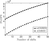
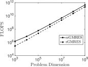
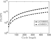
In Figure 1, we study the growth in estimated FLOP costs when all but one parameter are held fixed. For srGMRES, we again assume that $k=\frac{1}{2}m$ and that the total number of iterations needed for Algorithm 4.2 to converge is

$$j_{new}^{\eqref{algorithm.sgcrodr}}=\frac{n}{{10^{\frac{4}{9}+\frac{2m}{9m+9}}\log_{10}n}}.$$

This is somewhat arbitrary, but it qualitatively matches experimental observations. This formula is derived so that for the case that $n=10^{6}$ and for $m\rightarrow\infty$ we have that $j_{new}^{\eqref{algorithm.sgcrodr}}\rightarrow 100$ and the convergence is monotonically decreasing and relatively fast. It is necessary to have some assumption on the value of $j_{new}^{\eqref{algorithm.sgcrodr}}$ since Algorithm 4.2 has some overhead costs which need to be amortized over the total number of iterations. In the three graphs shown; we vary, respectively, number of shifts ($L$), problem dimension ($n$), and cycle length ($m$) with everything else being held constant. For the experiments in which $L$ is held constant, we chose $L=5$. Similarly, we chose $n=10^{7}$ and $m=100$ in the cases that these parameters were held constant.

We conclude by noting that we consider only one type of costs in this section. In reality, these methods also incur storage costs and data movement costs which are nontrivial for large-scale problems which must be considered. Furthermore, absent preconditioning, it is clear from the cost calculations that in the case of non-Hermitian shifted systems of the form treated in [20] that the method considered in that paper would be much cheaper than Algorithm 4.2, and absent preconditioning, for general non-Hermitian shifted linear systems satisfying the conditions in [13] (e.g., collinear residuals), that method would outperform Algorithm 4.1. Lastly, both Algorithms 4.1 and 4.2 can be used with flexible preconditioners with no additional computational or storage costs.

6 Numerical Results

We performed a series of numerical experiments to demonstrate the effectiveness of our algorithms as well as to compare performance (as measured in both matrix-vector product counts and CPU timings) with other algorithms. All tests were performed in Matlab R2014b (8.4.0.150421) 64-bit running on a Mac Pro workstation with two $2.26$ GHz Quad-Core Intel Xeon processors and 12 GB 1066 MHz DDR3 main memory. For these tests, we use two sets of QCD matrices downloaded from the University of Florida Sparse Matrix Library [9]. One set of matrices is a collection of seven $3072\times 3072$ complex matrices and the other is a collection of seven $49152\times 49152$ complex matrices. For each matrix $\mathbf{D}$ from the collection, there exists some critical value $\kappa_{c}$ such that for $\frac{1}{\kappa_{c}}<\frac{1}{\kappa}<\infty$, the matrix $\mathbf{A}=\frac{1}{\kappa}\mathbf{I}-\mathbf{D}$ is real-positive. For each $\mathbf{D}$, we took $\mathbf{A}=\left(\frac{1}{\kappa_{c}}+10^{-3}\right)\mathbf{I}-\mathbf{D}$ as our base matrix. In our experiments then, each set is taken as the sequence $\left\{\mathbf{A}_{i}\right\}$ and we solve a family of the form (2). As described in [9], the matrices $\mathbf{D}$ are discretizations of the Dirac operator used in numerical simulation of quark behavior at different physical temperatures. We note that larger real shifts of $\mathbf{A}_{i}$ yields better conditioned matrices for all $i$. For all experiments, we chose the right-hand side $\mathbf{b}_{1}=\mathbf{1}$, the vector of ones and set $\mathbf{b}_{i}=\mathbf{b}_{i-1}+\mathbf{d}_{i}$ where $\mathbf{d}_{i}$ is chosen randomly such that $\left\|\mathbf{d}_{i}\right\|=1e-1$. The requested relative residual tolerance was $\varepsilon=10^{-8}$. All augmentation was with harmonic Ritz vectors. For all experiments, we preconditioned with an incomplete LU-factorization (ILU) for the system with the smallest shift, constructed using the Matlab function ilu() called with the default Matlab settings. We comment that the usage of ILU was a matter of convenience and effectiveness for these sample problems. Its usage is meant to demonstrate proof-of-concept rather than as advocating the usage of ILU for large-scale QCD problems.

We also comment about methods which we have omitted from testing; the shifted restarted GMRES method [13], the shifted GMRES-DR method [8], and the recursive Recycled GMRES method for shifted systems proposed in [40]. We have omitted these methods from the tests as they do not admit general preconditioning. As such, they require substantially more iterations in many experiments. However, with the methods in [8, 13], there would be some number of shifts for which this method would be superior to those presented in this paper, as cost of recursion in our methods, even with preconditioning, would be greater than simply solving the unpreconditioned problems simultaneously with their shifted GMRES method [13].

Since these experiments involve solving shifted systems with shifts of varying magnitudes, it is useful to know information about the norms of our test matrices. Therefore, we provide both the one- and two-norms for these matrices (computed respectively with the Matlab functions norm($\cdot$, 1) and svds($\cdot$, 1)). The $1$-norms of these matrices all lie in the interval $\left(28,31\right)$, and their $2$-norms lie in the interval $\left(11,14\right)$.

In our first experiment, we tested Algorithm 4.2 with the smaller set of matrices for various recycle space dimension sizes and restart cycle lengths. We solve for shifts $\sigma\in\left\{.01,.02,.03,1,2,3\right\}$. We calculated total required matrix-vector products. We see in Table 4 that for these particular QCD matrices, good results can be achieved for a small recycled subspace dimension as long as the cycle length is sufficiently long.

Table 4: Matrix vector product counts for different pairs $(m,k)$ of restart cycle length and recycled subspace dimension for shifted Recycled GMRES. The matrices used in this experiment are the smaller set of QCD matrices from [9]. Experiments were performed for larger values than shown but no further improvement was observed

$m\backslash k$	$5$	$15$	$25$	$35$	$45$	$55$	$65$	$75$	$85$
5	1566	1295	1205	1161	1146	1131	1126	1116	1111
20	1466	1254	1182	1141	1122	1110	1107	1103	1096
35	1418	1229	1166	1132	1113	1103	1096	1095	1091
50	1363	1223	1158	1128	1114	1105	1099	1097	1090
65	1344	1219	1159	1124	1109	1106	1099	1090	1086
80	1321	1210	1153	1123	1109	1102	1098	1091	1085
95	1321	1210	1153	1124	1108	1100	1097	1093	1084

For the remaining tests, we use the larger set of QCD matrices. In Table 5 we compare time and matrix-vector product counts. For Algorithm 4.2, we chose cycle-length/recycle subspace dimension pair $(m,k)=(80,10)$ and use this pair for all experiments with Algorithm 4.2 except for the one shown in Figure 2. Parameters for Algorithm 4.1 and other tested methods were chosen in order to have the same per-cycle storage cost of $3k+2m=190$ vectors . For each family of linear systems, the experiment was performed ten times and the average time over these ten runs was taken as the run time. We solved for a larger number of shifts of varying magnitudes,

$$\sigma\in\left\{.001,.002,.003,.04,.05,.06,.07,.8,.9,1,1.1,10,11,12\right\}.$$

We compared four methods (Algorithm 4.1, Algorithm 4.2, sequentially applied GMRES and sequentially applied Recycled GMRES). We see that for this problem with these shifts, both proposed algorithms outperform the sequential applications of GMRES and Recycled GMRES both in terms of matrix-vector product counts and run times. In this case, the sGMRES algorithm is superior in time to srGMRES but not in terms of matrix-vector products, which demonstrates the difference in overhead costs.

Table 5: Timing (in seconds) and matrix-vector product (mat-vec) comparisons between preconditionedshifted rGMRES, shifted GMRES, and sequential applications of rGMRES with cycle length $m=80$ and recycled subspace dimension $k=10$ applied to the large QCD matrices. The same preconditioner was used in all experiments.

Method	mat-vecs	time
srGMRES	3117	358.44
sGMRES	4003	322.65
Seq. rGMRES	4379	469.78
Seq. GMRES	5665	489.16

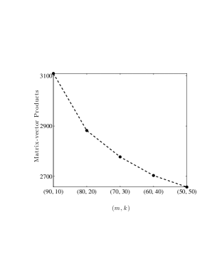
In Figure 2, for a total fixed augmented subspace dimension of $100$, we investigate how many matrix vector products are required to solve the same sequence of problems with the same shifts as in the previous experiment for different values of $(m,k)$ such that $m+k=100$ where $m$ is the dimension of the projected Krylov subspace and $k$ is the dimension of the recycled subspace. With this we demonstrate a reduction in iterations as we allow more information to be retained in the subspace.

\begin{picture}(0.0,0.0)\end{picture}

Fig. 2: Matrix-vector product counts for shifted Recycled GMRES for the sequence of large QCD amtrices and the same shifts as in Table 5. for various pairs $(m,k)$ of Krylov subspace dimension and recycled subspace dimension such that the total augmented subspace Krylov subspace dimension $m+k=100$.

In Table 6, we study matrix-vector product counts for different methods for shifts of varying magnitudes. For each shift, we solve just two systems, the base system and one shifted system. Thus we can see how many additional matrix-vector products are required for shifts of different magnitudes. What we see is that for this set of matrices, overall performance does not depend on shift magnitude. For larger shifts, we see that Algorithm 4.2 and sequentially applied rGMRES are comparable when there is only one shift. For the QCD matrices, larger real shifts produce better conditioned problems and Table 6 illustrates the trade-off between better conditioning and reduced effectiveness of the proposed algorithm for larger shifts. We hypothesize that the smallest values that are attained in the middle of the table are the result of Algorithms 4.1 and 4.2 still being effective for ${\mathcal{O}}(1)$ shifts where we also see improved conditioning of the shifted systems.

Table 6: Comparison of 3 methods for different shifts sizes. In each experiment, two systems were solved, the base system and one shifted system with the shift shown in the table column header.

Method\$\left\|\sigma\right\|$	$10^{-3}$	$10^{-2}$	$10^{-1}$	$10^{0}$	$10^{1}$	$10^{2}$	$10^{3}$
Sh. GMRES Alg. 4.1	1330	1405	1294	967	1067	1265	1306
Sh. rGMRES Alg. 4.2	980	1039	1017	804	908	1105	1144
Seq. rGMRES	1183	1170	1077	812	914	1111	1152

However, we have seen for larger numbers of shifts that Algorithm 4.2 can exhibit superior performance. This raises the question, what are the marginal costs of solving each additional linear system for Recycled GMRES and shifted Recycled GMRES, i.e., how many more matrix-vector products does each new shifted system require? This is investigated in Figure 3. For two sets of twenty shifts, we calculated the marginal cost of solving each additional shifted system using Algorithm 4.2 as compared to Recycled GMRES. In Figure 3 the first set of shifts (left-hand figure) were evenly space points from the interval $\left[0,1\right]$, and the second set of shifts (right-hand figure) were evenly spaced points from the larger interval $\left[1,10\right]$. In Figure 3,

\begin{picture}(0.0,0.0)\end{picture}

Fig. 3: Comparison of the marginal cost of solving each addition shifted system. For the left-hand figure, the shifts were evenly space points from the interval $\left[0,1\right]$, and in the right-hand figure, the shifts were evenly spaced points from the larger interval $\left[1,10\right]$

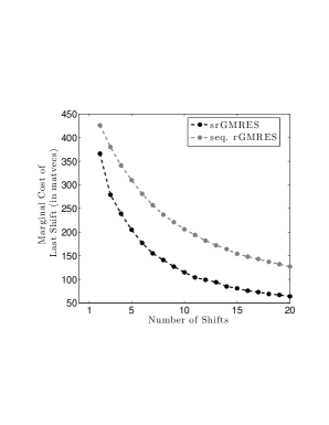
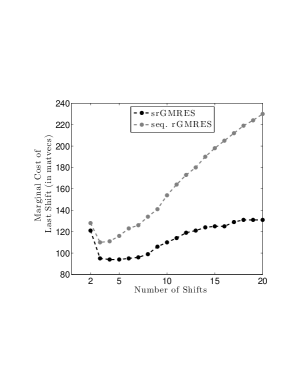
we see that for the smaller interval, the cost of each new shifted system drops for both algorithms but that Algorithm 4.2 has the lower marginal cost per shift. For the larger set of shifts, we see that the marginal costs for both algorithms actually increases for each new shift. However, the marginal cost of each new shifted system for Algorithm 4.2 becomes more stable (it levels off). For sequentially applied Recycled GMRES, the marginal costs increases steadily for all twenty shifts.

In Figure 4, we show the residual histories for systems solved using Algorithm 4.2 for shifts of various magnitudes,

$$\sigma\in\left\{10^{-3},10^{-2},10^{-1},1,10^{1},10^{2},10^{3}\right\}.$$

When viewing Figure 4, we see (in this example) that the amount of improvement

\begin{picture}(0.0,0.0)\end{picture}

Fig. 4: For the large QCD matrices and $(m,k)=(100,5)$, an illustration of the amount of residual improvement for different magnitude shifts, $\sigma\in\left\{10^{-3},10^{-2},\ldots,10^{3}\right\}$. In each subplot, we display the residual curves sequentially to reflect that the algorithm is called for each shifted linear system in sequence. The order in which the systems were solved is the same as the order of the listed shifts.

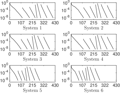
for the shifted residuals is somewhat predicted by the shift magnitude, though we again observe that the better conditioning of the systems with larger shifts seems to lead to more rapid convergence but at the expense of reduced effectiveness of the Lanczos-Galerkin projection.

Omitted here is a study of the eigendecomposition of the residuals, which yielded no discernible damping of certain eigenmodes or other interesting observable phenomena after the projection of the shifted residuals in our experiments. Such experiments were to investigate questions of the convergence rates observed in Figure 4.

7 Conclusions

We have presented two new methods for solving a family or a sequence of families of shifted linear systems with general preconditioning. These methods are derived from a general framework, which we also developed in this paper. These methods use subspaces generated during the minimum residual iteration of the base system to perform the projections for the shifted systems. This technique is fully compatible with right preconditioning, requiring only some additional storage. The strength of methods derived from this framework is that preconditioned methods for shifted systems easily can be built on top of existing minimum residual projection algorithms (and existing codes) with only minor modifications. We developed two algorithms: shifted GMRES and shifted Recycled GMRES. We demonstrated with numerical experiments that both methods can perform competitively.

Finally, we note that our framework is fully compatible with flexible and inexact Krylov subspace methods. As this work all follows from [6, 7, 19, 28], it is also clear that the method is also applicable to the case that we are solving (2) but with right-hand sides $\mathbf{b}_{i,\ell}$ which vary both with respect to coefficient matrix $\mathbf{A}_{i}$ and shift $\sigma_{\ell}$.

References

- [1] Mian Ilyas Ahmad, Daniel B. Szyld, and Martin B. van Gijzen, Preconditioned multishift BiCG for -optimal model reduction, Tech. Report 12-06-15, Department of Mathematics, Temple University, June 2012.
- [2] Allison H. Baker, Elizabeth R. Jessup, and Thomas Manteuffel, A technique for accelerating the convergence of restarted GMRES, SIAM Journal on Matrix Analysis and Applications, 26 (2005), pp. 962–984.
- [3] Tania Bakhos, Peter K. Kitanidis, Scott Ladenheim, Arvind Saibaba, and Daniel B. Szyld, Multipreconditioned gmres for shifted systems, In Preparation.
- [4] Manuel Baumann and Martin B. van Gijzen, Nested krylov methods for shifted linear systems, SIAM Journal on Scientific Computing, 37 (2015), pp. S90–S112.
- [5] Maria R. Celis, John E. Dennis, and Richard A. Tapia, A trust region strategy for nonlinear equality constrained optimization, in Numerical optimization, 1984 (Boulder, Colo., 1984), Paul T. Boggs, Richard H. Byrd, and Robert B. Schnabel, eds., SIAM, Philadelphia, PA, 1985, pp. 71–82.
- [6] Tony F. Chan and Michael K. Ng, Galerkin projection methods for solving multiple linear systems, SIAM J. Sci. Comput., 21 (1999), pp. 836–850.
- [7] Tony F. Chan and Wing L. Wan, Analysis of projection methods for solving linear systems with multiple right-hand sides, SIAM Journal on Scientific Computing, 18 (1997), pp. 1698–1721.
- [8] Dean Darnell, Ronald B. Morgan, and Walter Wilcox, Deflated GMRES for systems with multiple shifts and multiple right-hand sides, Linear Algebra and its Applications, 429 (2008), pp. 2415–2434.
- [9] Timothy A. Davis and Yifan Hu, The University of Florida sparse matrix collection, ACM Trans. Math. Softw., 38 (2011), pp. 1:1–1:25.
- [10] Eric de Sturler, Nested Krylov methods based on GCR, Journal of Computational and Applied Mathematics, 67 (1996), pp. 15–41.
- [11] , Truncation strategies for optimal Krylov subspace methods, SIAM Journal on Numerical Analysis, 36 (1999), pp. 864–889.
- [12] Andreas Frommer, for families of shifted linear systems, Computing, 70 (2003), pp. 87–109.
- [13] Andreas Frommer and Uwe Glässner, Restarted GMRES for shifted linear systems, SIAM Journal on Scientific Computing, 19 (1998), pp. 15–26.
- [14] Andreas Frommer, Stephan Güsken, Thomas Lippert, Bertold Nöckel, and Klaus Schilling, Many masses on one stroke: Economic computation of quark propagators, International Journal of Modern Physics C, 6 (1995), pp. 627–638.
- [15] André Gaul, Recycling Krylov subspace methods for sequences of linear systems: Analysis and applications, PhD thesis, Technischen Universität Berlin, 2014.
- [16] André Gaul, Martin H. Gutknecht, Jörg Liesen, and Reinhard Nabben, A framework for deflated and augmented Krylov subspace methods, SIAM Journal on Matrix Analysis and Applications, 34 (2013), pp. 495–518.
- [17] André Gaul and Nico Schlömer, Preconditioned recycling Krylov subspace methods for self-adjoint problems, Electronic Transactions on Numerical Analysis, 44 (2015), pp. 522–547.
- [18] Beat Jegerlehner, Krylov space solvers for sparse linear systems., Tech. Report IUHET-353, Indiana University, 1996.
- [19] Misha Kilmer, Eric Miller, and Carey Rappaport, QMR-based projection techniques for the solution of non-Hermitian systems with multiple right-hand sides, SIAM J. Sci. Comput., 23 (2001), pp. 761–780.
- [20] Misha E. Kilmer and Eric de Sturler, Recycling subspace information for diffuse optical tomography, SIAM Journal on Scientific Computing, 27 (2006), pp. 2140–2166.
- [21] Sabrina Kirchner, IDR-Verfahren zur Lösung von Familien geshifteter linearer Gleichungssysteme, master’s thesis, Bergische Universität Wuppertal, Department of Mathematics, Wuppertal, Germany, 2011.
- [22] Richard B. Lehoucq and Danny C. Sorensen, Deflation techniques for an implicitly restarted Arnoldi iteration, SIAM Journal on Matrix Analysis and Applications, 17 (1996), pp. 789–821.
- [23] Karl Meerbergen, The solution of parametrized symmetric linear systems, SIAM J. Matrix Anal. Appl., 24 (2003), pp. 1038–1059.
- [24] Ronald B. Morgan, GMRES with deflated restarting, SIAM Journal on Scientific Computing, 24 (2002), pp. 20–37.
- [25] Ronald B. Morgan and Min Zeng, Harmonic projection methods for large non-symmetric eigenvalue problems, Numerical Linear Algebra with Applications, 5 (1998), pp. 33–55.
- [26] Chris C. Paige, Beresford N. Parlett, and Henk A. van der Vorst, Approximate solutions and eigenvalue bounds from Krylov subspaces, Numerical Linear Algebra with Applications, 2 (1995), pp. 115–133.
- [27] Michael L. Parks, Eric de Sturler, Greg Mackey, Duane D. Johnson, and Spandan Maiti, Recycling Krylov subspaces for sequences of linear systems, SIAM Journal on Scientific Computing, 28 (2006), pp. 1651–1674.
- [28] Yousef Saad, On the Lanczos method for solving symmetric linear systems with several right-hand sides, Mathematics of Computation, 48 (1987), pp. 651–662.
- [29] , A flexible inner-outer preconditioned GMRES algorithm, SIAM Journal on Scientific Computing, 14 (1993), pp. 461–469.
- [30] , Iterative Methods for Sparse Linear Systems, SIAM, Philadelphia, Second ed., 2003.
- [31] Yousef Saad and Martin H. Schultz, GMRES: A generalized minimal residual algorithm for solving nonsymmetric linear systems, SIAM Journal on Scientific and Statistical Computing, 7 (1986), pp. 856–869.
- [32] Yousef. Saad, M. Yeung, J. Erhel, and Frèdèric Guyomarc’h, A deflated version of the conjugate gradient algorithm, SIAM Journal on Scientific Computing, 21 (2000), pp. 1909–1926. Iterative methods for solving systems of algebraic equations (Copper Mountain, CO, 1998).
- [33] Arvind K. Saibaba, Tania Bakhos, and Peter K. Kitanidis, A flexible Krylov solver for shifted systems with application to oscillatory hydraulic tomography, SIAM J. Sci. Comput., 35 (2013), pp. A3001–A3023.
- [34] Marcus Sarkis and Daniel B. Szyld, Optimal left and right additive Schwarz preconditioning for minimal residual methods with Euclidean and energy norms, Computer Methods in Applied Mechanics and Engineering, 196 (2007), pp. 1612–1621.
- [35] V. Simoncini, On the numerical solution of , BIT, 36 (1996), pp. 814–830.
- [36] Valeria Simoncini, Restarted full orthogonalization method for shifted linear systems, BIT. Numerical Mathematics, 43 (2003), pp. 459–466.
- [37] Valeria Simoncini and Daniel B. Szyld, Recent computational developments in Krylov subspace methods for linear systems, Numerical Linear Algebra with Applications, 14 (2007), pp. 1–59.
- [38] Kirk M. Soodhalter, Two recursive gmres-type methods for shifted linear systems with general preconditioning, arXiv 1403.4428v2, 2014.
- [39] Kirk M. Soodhalter, Block krylov subspace recycling for shifted systems with unrelated right-hand sides, SIAM Journal on Scientific Computing (To Appear), (2016).
- [40] Kirk M. Soodhalter, Daniel B. Szyld, and Fei Xue, Krylov subspace recycling for sequences of shifted linear systems, Applied Numerical Mathematics, 81C (2014), pp. 105–118.
- [41] Shun Wang, Eric de Sturler, and Glaucio H. Paulino, Large-scale topology optimization using preconditioned Krylov subspace methods with recycling, International Journal for Numerical Methods in Engineering, 69 (2007), pp. 2441–2468.
- [42] Gang Wu, Yan-Chun Wang, and Xiao-Qing Jin, A preconditioned and shifted GMRES algorithm for the PageRank problem with multiple damping factors, SIAM J. Sci. Comput., 34 (2012), pp. A2558–A2575.