Nucleon form factors for the elastic electron-deuteron scattering at high momentum transfer

Abstract

The reaction of the elastic electron-deuteron scattering at high momentum transfer is investigated within the Bethe-Salpeter approach. The relativistic covariant Graz II separable kernel of nucleon-nucleon interactions is used to analyze the deuteron structure functions, form factors and tensor of polarization components. The modern data for the electromagmetic nucleons structure from the double polarization experiments as well as some other models of the nucleon form factors are considered.

74.50.+r, 74.80.Fp

1 Introduction

The deuteron being the simplest two-nucleon bound system is a powerful instrument to study strong interactions. The reaction of elastic electron-deuteron scattering provides information not only on NN interaction but also on the electromagnetic structure of nucleons. Such investigations at high energies are of great interest nowadays, especially in the context of future experiments at being upgraded JLab facilities.

It is necessary to note that in order to describe the elastic form factors of the deuteron at high momentum transfer ($Q^{2}=-q^{2}>2$ (GeV/c)²) the relativistic properties of the strong interactions should be taken into account. Here, properties of core nuclear forces play a very important role. From the physical point of view, elastic electron-deuteron scattering at transfer momentum up to 6 (GeV/c)² is an amazing phenomenon taking into account that binding energy of the deuteron is very small (2.2 MeV). So the subject of investigation has a great significance for the nuclear and particle physics.

Some approaches, based on the Bethe-Salpeter (BS) equation [1], satisfy this condition, among them are the light-front dynamics [2], the equal-time equation [3], BS approach with separable interaction [4] and so on. In the last approach, one has to solve the system of linear integral equations for both the NN scattered states and the bound state – the deuteron. In order to find a solution of a system of integral equations, it is a good idea to use a separable ansatz [4] for the interaction kernel in the BS equation. Then, one can transform the integral equations into a system of algebraic linear ones which can be solved. Parameters of the interaction kernel are extracted from an analysis of phase shifts for respective partial-wave states and low-energy parameters as well as deuteron properties (bound state energy, magnetic moment, elastic form factors etc.). In the Refs. [5] and [6] the latter approach was developed and applied to the reaction of the deuteron electrodisintegration.

The electromagnetic (EM) structure of nucleons at high momentum transfer is another topic of interest. In the paper, four models for the nucleon form factors are used. First of them – the dipole fit (DFF) [7] – was widely used. The main feature of this model is that the ratio of electric $G^{\rm E}_{\rm p}$ and magnetic $G^{\rm M}_{\rm p}$ proton form factors is constant. Another one – the relativistic harmonic oscillator model (RHOM) [8] – is the quark model with a relativistic harmonic oscillator potential.

However, recently there was an intensive discussion that the ratio obtained by the Rosenbluth separation technique differs from the one obtained by the recoil polarization method [9, 10]. To describe the results of the latter method, it is necessary to use a certain parametrization of the ratio as some linear function of the transfer momentum squared. The model with described ratio for the electric proton form factor and the Galster parametrization [11] for the neutron electric form factor – modified dipole fit (MDFF1) - is also considered (see also, [12] and [6]).

Recently the Unitary and Analytic (U&A) approach has been used to develop new nine-resonance model [13]. This model which includes new experimental data on the nucleon EM form factors as well as a new method of introducing the asymptotic behavior for the EM form factors also used in calculations.

In contrast to the Ref. [14], the influence of the new parametrization of proton electric form factor is investigated, and in the development of our previous papers [15] and [16], the deuteron form factors are calculated at high energies where the analytic structure of the vertex functions should be taken into account.

Also we have considered high-energy dynamics of the poles contributions which arise from the analytic structure of the separable kernel.

The paper is organized as follows: in Sec.2 we describe the models of the nucleon form factors and consider analytic structure of the deuteron EM current in the Sec.3. The obtained results are discussed in Sec.4. In Sec.5 the conclusion is given.

2 Models of the nucleon form factors

We calculate elastic electron-deuteron scattering in the relativistic impulse approximation within the BS approach with the covariant Graz II (rank III) kernel of the NN interaction [17] and [14].

Details of the calculations of the deuteron structure functions $A(q^{2})$, $B(q^{2})$, charge $F_{\rm C}(q^{2})$, quadrupole $F_{\rm Q}(q^{2})$ and magnetic $F_{\rm M}(q^{2})$ form factors and tensor polarization components $T_{20}$, $T_{21}$ of the final deuteron can be found in [15].

We use four models of the electromagnetic nucleon form factors (see also, [7], [12], [13] and  [8]):

• the original dipole fit for the proton and neutron form factors (DFF) is

  $$F_{d}=(1+Q^{2}/0.71)^{-2},$$

  $$G_{\rm E}^{\rm p}=F_{d},\hskip 42.67912ptG_{\rm E}^{\rm n}=0,$$

  $$G_{\rm M}^{\rm p}=\mu_{\rm p}G_{\rm E}^{\rm p},\hskip 28.45274ptG_{\rm M}^{\rm n}=\mu_{\rm n}G_{\rm E}^{\rm p};$$ (1)

• the modified dipole fit 1 (MDFF1) is

  $$G_{\rm E}^{\rm p}=(1-0.13(Q^{2}-0.04))F_{d},$$

  $$G_{\rm E}^{\rm n}=-\frac{\mu_{n}\tau}{1+5.6\tau}F_{d},$$

  $$G_{\rm M}^{\rm p}=\mu_{\rm p}F_{d},$$

  $$G_{\rm M}^{\rm n}=\mu_{\rm n}F_{d}.$$ (2)

  In MDFF1 we take into account the latest JLab data [9] for the proton electric form factor by the following ratio $\mu_{p}G_{\rm E}^{\rm p}/G_{\rm M}^{\rm p}=1-0.13(Q^{2}-0.04)$, while for the neutron electric form factor we use the Galster [11] parametrization.

• the proposed nine-resonance U&A model of the nucleon has 12 free parameters. Their values were obtained from the analysis of the existent experimental data and additionally new one measured recently in Mainz. All details and formulas can be found in Ref. [13].

• the relativistic harmonic oscillator is

  $$I^{(3)}=\frac{1}{(1+Q^{2}/2m^{2})^{2}}$$

  $$\times\exp{\frac{1}{2\cdot 0.42}\frac{-Q^{2}}{1+Q^{2}/2m^{2}}},$$

  $$G_{\rm E}^{\rm p}=I^{(3)},$$

  $$G_{\rm E}^{\rm n}=Q^{2}/2m^{2}I^{(3)},$$

  $$\frac{G_{\rm M}^{\rm p}}{\mu_{\rm p}}=\frac{G_{\rm M}^{\rm n}}{\mu_{\rm n}}=I^{(3)}.$$ (3)

  The relativistic harmonic oscillator model is based on the quark model with the relativistic oscillator potential. All the FFs calculated in this model have the correct asymptotic behavior. The only free parameter in the model is the oscillator parameter which was found from fitting of the experimental data.

Above $\mu_{\rm p}=2.7928$ and $\mu_{\rm n}=-1.9130$ are the magnetic moments of the nucleons, $Q^{2}=-q^{2}>0$ is the transfer momentum squared, $\tau=Q^{2}/4m^{2}$, $m$ is the nucleon mass, and all dimensional parameters are in (GeV/c)².

3 Analytic structure

After the partial-wave decomposition the matrix element of the deuteron current has the following form

$$\langle D^{\prime}{\cal M}^{\prime}|j_{\mu}|D{\cal M}\rangle={\cal I}_{1\;\mu}^{{\cal M}^{\prime}{\cal M}}(q^{2})\;F_{1}^{\rm(S)}(q^{2})+$$

$$+{\cal I}_{2\;\mu}^{{\cal M}^{\prime}{\cal M}}(q^{2})\;F_{2}^{\rm(S)}(q^{2}),$$ (4)

$${\cal I}_{1,2\;\mu}^{{\cal M}^{\prime}{\cal M}}(q^{2})=i\int dp_{0}\;|\textbf{p}|^{2}\;d|\textbf{p}|\;d(\cos{\theta})$$

$$\times\sum_{L\prime,L=0,2}\;\phi_{L\prime}(p_{0}^{\prime},|\textbf{p}^{\prime}|)\phi_{L}(p_{0},|\textbf{p}|)$$

$$\times I^{L^{\prime},L}_{1,2\;{\cal M^{\prime}}{\cal M}\;\mu}(p_{0},|\textbf{p}|,\cos{\theta},q^{2}),$$

where the function $I^{L^{\prime},L}_{1,2\;{\cal M^{\prime}}{\cal M}\;\mu}(p_{0},|\textbf{p}|,\cos{\theta},q^{2})$ is the result of the trace calculations. The radial part of the amplitude is

$$\phi_{L}(p_{0},|\textbf{p}|)=S_{++}(p_{0},|\textbf{p}|)g_{L}(p_{0},|\textbf{p}|),$$ (5)

with $g_{L}(p_{0},|\textbf{p}|)$ being the radial part of the vertex function and

$$S_{++}(p_{0},|\textbf{p}|)=\frac{1}{(M_{d}/2+p_{0}-E_{\textbf{p}})(M_{d}/2-p_{0}-E_{\textbf{p}})},$$ (6)

being the positive energy part of the propagators and the energy $E_{\textbf{p}}=\sqrt{m^{2}+\textbf{p}^{2}}$.

Analyzing the analytic structure of expressions (5) and (6) we can write the following expression for the poles in the $p_{0}$ complex plane:

• initial deuteron

  for propagator $S_{++}(p_{0},|\textbf{p}|)$:

  $${\bar{p}_{0}}=\pm M_{d}/2\mp E_{\textbf{p}}\pm i\epsilon,$$ (7)

  for functions $g_{L}(p_{0},|\textbf{p}|)$:

  $${\bar{p}_{0}}=\pm E_{\beta_{k}}\mp i\epsilon,$$ (8)

• final deuteron

  for propagator $S_{++}(p_{0}^{\prime},|\textbf{p}^{\prime}|)$:

  $${\bar{p}_{0}}=-(1+4\eta)M_{d}\pm$$

  $$\pm\sqrt{E_{\textbf{p}}^{2}+4\xi M_{d}|\textbf{p}|\cos{\theta}+4\xi^{2}M_{d}^{2}}\mp i\epsilon,$$ (9)

  for functions $g_{L^{\prime}}(p_{0}^{\prime},|\textbf{p}^{\prime}|)$:

  $${\bar{p}_{0}}=-\eta M_{d}\pm$$

  $$\sqrt{E_{\beta_{k}}^{2}+2\xi M_{d}|\textbf{p}|\cos{\theta}+\xi^{2}M_{d}^{2}}\mp i\epsilon,$$ (10)

with the energy $E_{\beta_{k}}=\sqrt{\beta_{k}^{2}+\textbf{p}^{2}}$, $\eta=Q^{2}/4M_{d}^{2}$ and $\xi=\sqrt{\eta(1+\eta)}$.

To calculate the matrix elements (4) we should perform the Wick rotation procedure. However, during the used procedure, the poles (9) and (10) can get into the contour of the $p_{0}$ integration. Additionally, the residue in these poles should be taken into account. All contributions from the poles have the threshold value on $Q^{2}$ which have the following form:

for the propagator $S_{++}(p_{0}^{\prime},|\textbf{p}^{\prime}|)$:

$$Q_{0}^{2}=M_{d}(2m-M_{d}),$$

for the functions $g_{L^{\prime}}(p_{0}^{\prime},|\textbf{p}^{\prime}|)$:

$$Q^{2}_{k}=4M_{d}\beta_{k}.$$

The Wick rotation procedure can be written as:

$$i\int\limits_{-\infty}^{\infty}fdp_{0}=\int\limits_{-\infty}^{\infty}fdp_{4}-$$

$$-2\pi\sum_{k}{\theta(Q^{2}-Q_{k}^{2})\;Res_{k}(f,p_{0}=\bar{p}_{0}^{k})},$$ (11)

where the threshold values $Q_{k}^{2}$ for the Graz II kernel are in table 1.

$k$	$Q^{2}_{k}$ (GeV/c)2
0	0.004
1	1.182
2	1.736
3	3.915
4	5.965

Table 1: Table 1. Threshold values for the poles of the kernel

It is seen that calculations with the $Q^{2}>1.182$ (GeV/c)² must take into account contribution from the poles of vertex function.

4 Results and discussion

Figs. 1-6 show the influence of the considered models of the nucleon electromagnetic form factors to the elastic electron-deuteron scattering at high momentum transfer.

In Fig. 1 the deuteron structure function $A(q^{2})$ is shown. It is seen that the difference between considered models is significant and at the $Q^{2}=10$ (GeV/c)² it reaches the value of about 2 orders for the Ref. [13] and RHOM models. We can also see that the best model up to $Q^{2}=3$ (GeV/c)² is RHOM model in context of experimental data coincidence, but in high-energy region the result is overestimated. Also the results show interesting transition in MDFF1 behavior, it behaves like DFF up to $Q^{2}=3$ (GeV/c)² and demonstrates the similar behavior with the [13] model past $Q^{2}=6$ (GeV/c)².

The deuteron structure function $B(q^{2})$ is plotted in Fig. 2. The DFF and MDFF1 results practically coincide till $Q^{2}=10$ (GeV/c)². The RHOM and [13] models are significantly differ from previous ones and each other. The [13] have a node at approximately $Q^{2}=6.5$ (GeV/c)² which can be explained by the node in the proton electric $G_{\rm E}^{\rm p}$ FF at $Q^{2}\sim 11-12$ (GeV/c)². Unfortunately there is no high-energy data for the $B(q^{2})$ structure function to make any suggestions about the physicality of such behavior.

In Figs. 3 and 4 the deuteron charge $F_{\rm C}(q^{2})$ and quadrupole $F_{\rm Q}(q^{2})$ form factors are shown. Like for the $A(q^{2})$ and $B(q^{2})$ structure functions result of the RHOM model lies much higher than other results. The MDFF1 model demonstrates the some specific feature in behavior of $F_{\rm C}(q^{2})$ where another one node appears at the $Q^{2}=8.5$ (GeV/c)² which corresponds to the node in the proton electric $G_{\rm E}^{\rm p}$ FF. As for $F_{\rm Q}(q^{2})$ MDFF1 shows the same transition like in the $A(q^{2})$ structure function case.

The tensor component $T_{20}$ are shown in the Fig 5. It is seen that all 4 models practically coincide up to $Q^{2}=4$ (GeV/c)² and [13] coincides with RHOM up to $Q^{2}=8.5$ (GeV/c)².

The $T_{21}$ are shown in the Fig 6. It is seen that all results are similar up to $Q^{2}=1$ (GeV/c)² only. Let note that [13] coincides with RHOM up to $Q^{2}=5.5$ (GeV/c)² and DFF, MDFF1 up to $Q^{2}=4.0$ (GeV/c)²

It should be noted that results for tensor components $T_{20}$ and $T_{21}$ can be combined into two groups until the $Q^{2}=4-4.5$ (GeV/c)² where DFF and MDFF1 models in first pair and [13] and RHOM in second pair have a very similar behavior. However in the region with higher energy all four models show very different trend.

Fig. 7 represents the influence of the vertex function poles to the full integral value. It is seen that past $Q^{2}=2$ (GeV/c)² the poles begin to play an important role. It is surprising that for the $B(q^{2})$ structure function at the $Q^{2}=4.5$ (GeV/c)² contribution of the poles of the separable kernel become crucial, while for the $A(q^{2})$ their contribution hardly reach $25\%$ on the whole interval. The result for the function $B(q^{2})$ is because the contributions for the $3D$- and $2D_{1}$-integrals (see Eq. (11)) have different signs and their sum become much smaller then contribution of the residue in the poles of deuteron vertex function.

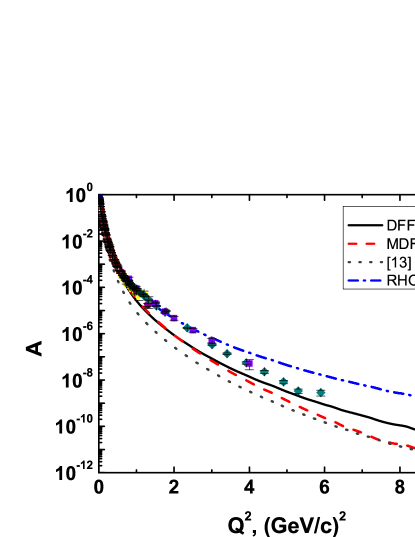
Figure 1: Fig.1. The deuteron structure function $A(q^{2})$ as a function of the transfer momentum squared. Calculations with DFF (black solid line), MDFF1 (dashed red line),  [13] (gray dotted line) and RHOM (blue dashed dotted line) nucleon form factors are shown. Experimental data are taken from [18].

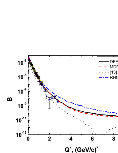
Figure 2: Fig.2. As in Fig.1, but for the structure function $B(q^{2})$. Experimental data are taken from [19] and [20].

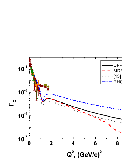
Figure 3: Fig.3. As in Fig.1, but for the charge form factor $F_{\rm C}(q^{2})$. Experimental data are taken from [21].

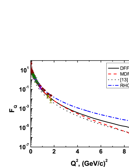
Figure 4: Fig.4. As in Fig.1, but for the quadrupole form factor $F_{\rm Q}(q^{2})$. Experimental data are taken from [21].

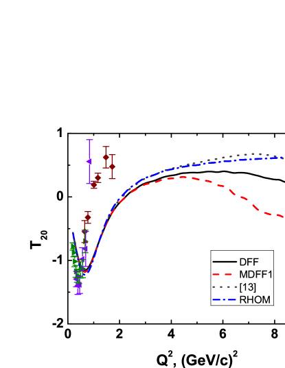
Figure 5: Fig.5. As in Fig.1, but for the tensor polarization component $T_{20}(q^{2})$. Experimental data are taken from [21].

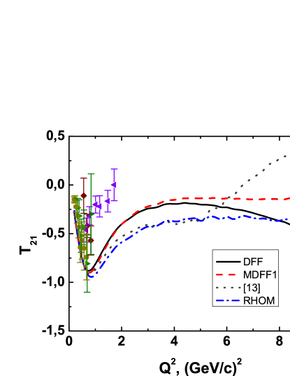
Figure 6: Fig.6. As in Fig.1, but for the tensor polarization component $T_{21}(q^{2})$. Experimental data are taken from [21].

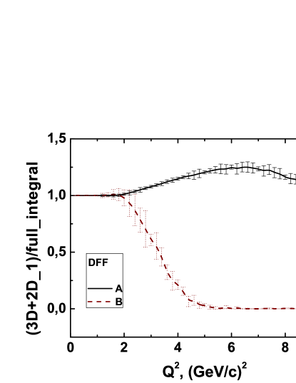
Figure 7: Fig.7. $3D+2D_{1}$-integral contribution to the full result.

5 Conclusion

In the paper the elastic electron-deuteron scattering in the relativistic impulse approximation within the Bethe-Salpeter approach with the covariant Graz II kernel of the nucleon-nucleon interaction is considered. Calculations are performed at high momentum transfer up to 10 (GeV/c)². The analytic structure of the vertex functions are taken into account. The result of calculations with four models of the nucleon form factors are compared. It is necessary to stress that considered high energies are required to take into account relativistic properties of the deuteron.

As for the significant change between nucleon form factors models there is a lack of experimental data to make any statements about which model is closer to real physics.

The difference between presented theoretical calculations and experimental data can be explained as it is necessary to take into account additional contributions. Thus, the next step is to use the modern separable kernel of nucleon-nucleon interaction [5]. As an extension to the calculations, some effects should be taken into account. Among them are the relativistic P-states in the deuteron, two-body interaction currents and off-mass shell nucleon effects (see, e.g. [4], [22]). As concerning off-mass shell effects in this approach, there is a possibility to solve inverse task and to determine the behavior of nucleon form factors of bound nucleon.

References

- [1] E. E. Salpeter and H. A. Bethe, Phys. Rev. 84, 1232 (1951).
- [2] J. Carbonell, V.A. Karmanov, PoS LC2010 (2010) 014, arXiv:1009.4522 [hep-ph]; J. Carbonell, V.A. Karmanov, Eur. Phys. J. A 46 (2010) 387.J. Carbonell, V.A. Karmanov, Nucl.Phys. A663 (2000) 361-364.
- [3] V. Pascalutsa and J. A. Tjon, Phys. Lett. B435, 245 (1998) [nucl-th/9711005].
- [4] S.G. Bondarenko et al., Prog. Part. Nucl. Phys.48, 449 (2002) [nucl-th/0203069]
- [5] S. G. Bondarenko et al., Nucl. Phys. A832, 233 (2010) [arXiv:0810.4470 [nucl-th]]; S. G. Bondarenko et al., Nucl. Phys. A848, 75 (2010) [arXiv:1002.0487 [nucl-th]]; S. G. Bondarenko, V. V. Burov and E. P. Rogochaya, Phys. Lett. B705, 264 (2011); S. G. Bondarenko, V. V. Burov and E. P. Rogochaya, Nucl. Phys. Proc. Suppl. 219-220, 126 (2011) [arXiv:1108.4170 [nucl-th]]; S. G. Bondarenko, V. V. Burov and E. P. Rogochaya, Nucl. Phys. Proc. Suppl. 245, 291 (2013).
- [6] S. G. Bondarenko, V. V. Burov and E. P. Rogochaya, Few Body Syst. 49, 121 (2011) [arXiv:1008.0107 [nucl-th]].
- [7] H. Pietschmann and H. Stremnitzer, Lett. Nuovo Cim. 2S1, 841 (1969) [ Lett. Nuovo Cim. 2, 841 (1969)].
- [8] V. V. Burov et al., Europhys. Lett. 24, 443 (1993) [hep-ph/9310377].
- [9] O. Gayou et al. [Jefferson Lab Hall A Collaboration], Phys. Rev. Lett. 88, 092301 (2002) [nucl-ex/0111010].
- [10] M. K. Jones et al. [Jefferson Lab Hall A Collaboration], Phys. Rev. Lett. 84, 1398 (2000) [nucl-ex/9910005].
- [11] S. Galster et al., Nucl. Phys. B32, 221 (1971).
- [12] K. S. Egiyan et al. [CLAS Collaboration], Phys. Rev. Lett. 98, 262502 (2007) [nucl-ex/0701013].
- [13] C. Adamuscin et al., Nucl. Phys. Proc. Suppl. 245, 69 (2013).
- [14] G. Rupp and J. A. Tjon, Phys. Rev. C41, 472 (1990).
- [15] S. G. Bondarenko, V. V. Burov and S. M. Dorkin, Phys. Atom. Nucl. 63, 774 (2000) [Yad. Fiz. 63, 844 (2000)].
- [16] A. Bekzhanov, S. Bondarenko and V. Burov, Nucl. Phys. Proc. Suppl. 245, 65 (2013).
- [17] L. Mathelitsch, W. Plessas and W. Schweiger, Phys. Rev. C26, 65 (1982);
- [18] C. D. Buchanan and M. R. Yearian, Phys. Rev. Lett. 15, 303 (1965); D. Benaksas, D. Drickey and D. Frerejacque, Phys. Rev. 148, 1327 (1966); J. E. Elias et al., Phys. Rev. 177, 2075 (1969); S. Galster et al., Nucl. Phys. B32, 221 (1971); R. G. Arnold et al., Phys. Rev. Lett. 35, 776 (1975); G. G. Simon, C. Schmitt and V. H. Walther, Nucl. Phys. A364, 285 (1981); R. Cramer et al., Z. Phys. C29, 513 (1985); S. Platchkov et al., Nucl. Phys. A510, 740 (1990); L. C. Alexa et al. [Jefferson Lab Hall A Collaboration], Phys. Rev. Lett. 82, 1374 (1999) [nucl-ex/9812002]; D. Abbott et al. [Jefferson Lab t(20) Collaboration], Phys. Rev. Lett. 82, 1379 (1999) [nucl-ex/9810017].
- [19] C. D. Buchanan and M. R. Yearian, Phys. Rev. Lett. 15, 303 (1965); G. G. Simon, C. Schmitt and V. H. Walther, Nucl. Phys. A364, 285 (1981); S. Auffret et al., Phys. Rev. Lett. 54, 649 (1985); R. Cramer et al., Z. Phys. C29, 513 (1985); R. G. Arnold et al., Phys. Rev. C42, 1 (1990).
- [20] R. Suleiman, Ph.D. thesis, Kent State University (1999).
- [21] D. Abbott et al. [JLAB t20 Collaboration], Eur. Phys. J. A7, 421 (2000) [nucl-ex/0002003]; D. M. Nikolenko et al., Phys. Rev. Lett. 90, 072501 (2003); C. Zhang et al., Phys. Rev. Lett. 107, 252501 (2011).
- [22] S.G. Bondarenko et al., PEPAN Letters 5(128), 17 (2005).