The physics of the optical light curve in supernovae

Abstract

We present a new formula which models the rate of decline of supernovae (SN) as given by the light curve in various bands. The physical basis is the conversion of the flux of kinetic energy into radiation. The two main components of the model are a power law dependence for the radius–time relation and a decreasing density with increasing distance from the central point. The new formula is applied to SN 1993J, SN 2005cf, SN 1999ac, and SN 2001el in different bands.

Keywords: Interstellar medium (ISM) and nebulae in the Milky Way, Supernova remnants,

1 Introduction

The light curve (LC) of supernovae (SN) at a given wavelength $\lambda$ denotes the luminosity–time relation. The astronomers work in terms of apparent/absolute magnitude and therefore the LC in SN is usually presented as a magnitude versus time relation. We have two great astronomical classifications for the LC: type I SN and type II SN. The type I has a fast decrease in magnitude followed by a nearly linear increase. In luminosity terms, the SN has a fast increase followed by a nearly exponential decay. The type II has a fast decrease in magnitude followed by oscillations, type IIb, or a plateau, type IIp; a decay follows the plateau. In this complex morphology, we will always specify the type of SN under consideration. The luminosity is usually modeled by the formula

$$L=L_{\lambda,0}\exp(-\frac{t}{\tau})\quad,$$ (1)

where $L$ and $L_{\lambda,0}$ are the luminosity at time $t$ and at $t=0$ respectively, and $\tau$ is the typical lifetime, see Bowers and Deeming (1984). As an example, the radioactive isotope ⁵⁶Ni has $\tau$ = 8.767 days. On introducing the apparent magnitude $m_{\lambda}$, the previous formula becomes

$$m_{\lambda}=k^{\prime}_{\lambda}+1.0857(\frac{t}{\tau})\quad,$$ (2)

where $k^{\prime}_{\lambda}$ is a constant. The absolute magnitude $M_{\lambda}$ scales in the same way:

$$M_{\lambda}=k^{\prime\prime}_{\lambda}+1.0857(\frac{t}{\tau})\quad,$$ (3)

where $k^{\prime\prime}_{\lambda}$ is another constant. The observational fact that, as an example, in IC 4182 the LC has a half-life of 56 days, requires the production of ⁵⁶Co, see van Hise (1974). The previous formula is an empirical relation which is based solely on observations rather than theory. The theory for SNII LCs was first developed by Grasberg et al. (1971) and later analytically and numerically explored by Falk and Arnett (1973); Arnett (1980); Arnett and Fu (1989). A model for the luminosity in $H\alpha$ of supernovae as a function of time can be found in Figure 7 of Chevalier and Fransson (1994). The LCs of type Ia SN have been explained (including the secondary maximum) by a time-dependent multigroup radiative transfer calculation, see Kasen (2006). A model for type II supernovae explosions has been built including progenitor mass, explosion energy, and radioactive nucleosynthesis, see Kasen and Woosley (2009). The model atmosphere code PHOENIX was used to calculate type Ia supernovae, see Jack et al. (2011). The previous works leave a series of questions unanswered or merely partially answered.

• Given the observational fact that the radius–time relation in young SNRs follows a power law, is it possible to find a theoretical law of motion which fits the observations?

• Can a model of an expansion in the framework of the thin layer approximation produce the observed radius–time relation?

• Can we express the flux of kinetic energy in the framework of an approximate law of motion and a medium characterized by a decreasing density?

• Can we parametrize the conversion of the flux of kinetic energy into total observed luminosity?

• Can we parametrize the fraction of conversion of the total luminosity into the optical bands?

In order to answer these questions, in Section 2.2 we analyze the existing equations of motion for SN 1993J as well a new adjustable equation. Section 3 reviews the basic formulas of synchrotron emission and reports the conversion of flux of kinetic energy into an observed band. Section 4 reports the application of the new formulas to different SNs in various bands.

2 The equation of motion

This section reviews three existing parameters for SNRs, the power law model and a new solution in the framework of the thin layer approximation.

2.1 Some existing solutions

The Sedov–Taylor solution is

$$R(t)=\left({\frac{25}{4}}\,{\frac{{\it E}\,{t}^{2}}{\pi\,\rho}}\right)^{1/5}\quad,$$ (4)

where $E$ is the energy injected into the process and $t$ is time, see Sedov (1944); Taylor (1950a, b); Sedov (1959); McCray (1987). Our astrophysical units are: time, ($t_{1}$), which is expressed in years; $E_{51}$, the energy in $10^{51}$ erg; $n_{0}$, the number density expressed in particles $\mathrm{cm}^{-3}$  (density $\rho=n_{0}$m, where m = 1.4$m_{\mathrm{H}}$). In these units, Equation (4) becomes

$$R(t)\approx 0.313\,\sqrt[5]{{\frac{{\it E_{51}}\,{{\it t_{1}}}^{2}}{{\it n_{0}}}}}~{}{pc}\quad.$$ (5)

The Sedov–Taylor solution scales as $R(t)\approx t^{2/5}=t^{0.4}$.

A second solution is connected with momentum conservation in the presence of a constant density medium, see Dyson, J. E. and Williams, D. A. (1997); Padmanabhan (2001); Zaninetti (2009). The astrophysical radius in pc as a function of time is

$$R(t)=\sqrt[4]{{{\it R_{0}}}^{3}\left(4.08\,10^{-6}\,{\it v_{1}}\,\left(t_{1}-t_{{0}}\right)+{\it R_{0}}\right)}\,\mathrm{pc}\quad,$$ (6)

where $t_{1}$ and $t_{0}$ are the time in years, $R_{0}$ is the radius in pc when $t_{1}=t_{0}$, and $v_{1}$ is the velocity in km s^-1 when $t_{1}=t_{0}$. The thin layer solution in the presence of a constant density medium scales as $t^{0.25}$. A relativistic solution of the thin layer approximation can be found in Zaninetti (2010).

A sophisticated approach as given by Chevalier (1982a) and Chevalier (1982b) analyzes self-similar solutions with varying inverse power law exponents for the density profile of the advancing matter, $R^{-n}$, and ambient medium, $R^{-s}$. The previous assumptions give a law of motion $R\propto t^{\frac{n-3}{n-s}}$ when $n\,>5$.

2.2 The equation of motion as a power law

The equation of the expansion of an SNR can be modeled by a power law of the type

$$R(t)=R_{0}(\frac{t}{t_{0}})^{\alpha}\quad,$$ (7)

where $R$ is the radius of the expansion, $t$ is the time, $R_{0}$ is the radius at $t=t_{0}$, and $\alpha$ is an exponent which can be found from a numerical analysis. In order to find the unknown parameters, we analyzed the data of supernova SN 1993J , classified as type IIb, which began to be visible in M81 in 1993, see Ripero et al. (1993), and presented a circular symmetry for 4000 days, see Marcaide et al. (2009). Its distance is 3.63 Mpc (the same as M81), see Freedman et al. (1994).

The velocity is

$$V(t)=\alpha R_{0}(\frac{1}{t_{0}})^{\alpha}t^{(\alpha-1)}\quad.$$ (8)

As an example, Figure 1 reports the fit of SN 1993J . We have chosen this SN because:

• it presents a nearly spherical expansion,

• the temporary radius of expansion has been measured for $\approx$ 10 yr in the radio band, seeMarcaide et al. (2009).

The observed radius–time relation of SN 1993J allows us to calibrate our model and the application of the least squares method through the FORTRAN subroutine LFIT from Press et al. (1992) allows finding $\alpha$ = 0.828  . Therefore the radius is growing more slowly than a free expansion with constant velocity, $R\propto\,t$, but more quickly than the Sedov–Taylor solution, $R\propto t^{0.4}$, see Equation (4).

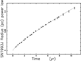
Figure 1: The theoretical radius as given by the power law fit represented by Equation (7) with $\alpha$ =0.828, $R_{0}$=0.0087 pc and $t_{0}$ = 0.498 yr. The astronomical data of SN 1993J are represented by vertical error bars and are extracted from Table 1 in Marcaide et al. (2009).

2.3 An adjustable equation of motion

We assume that around the SNR the density of the interstellar medium (ISM) has the following two piecewise dependencies

$$\rho(R)=\left\{\begin{array}[]{ll}\rho_{0}&\mbox{if $R\leq R_{0}$ }\\ \rho_{0}(\frac{R_{0}}{R})^{d}&\mbox{if $R>R_{0}$ ~{}.}\end{array}\right.$$ (9)

This assumption allows us to set up the initial conditions, otherwise the dependence $\rho(R)\propto(\frac{R_{0}}{R})^{d}$ will have a pole at $R=0$. At the moment of writing there is not a clear determination of the gradients around the SN and therefore $d$ can be considered a free parameter.

In this framework the SN is moving and the density, which is at rest, decreases as an inverse power law with an exponent $d$ which can be fixed from the observed temporal evolution of the radius. The mass swept, $M_{0}$, in the interval $0\leq r\leq R_{0}$ is

$$M_{0}=\frac{4}{3}\,\rho_{{0}}\pi\,{R_{{0}}}^{3}\quad.$$ (10)

The mass swept, $M$, in the interval $0\leq r\leq R$ with $r\geq R_{0}$ is

$$M=-4\,{r}^{3}\rho_{{0}}\pi\,\left({\frac{R_{{0}}}{r}}\right)^{d}\left(d-3\right)^{-1}+4\,{\frac{\rho_{{0}}\pi\,{R_{{0}}}^{3}}{d-3}}+\frac{4}{3}\,\rho_{{0}}\pi\,{R_{{0}}}^{3}\quad.$$ (11)

Momentum conservation in the thin layer approximation requires that

$$Mv=M_{0}v_{0}\quad,$$ (12)

where $v$ is the velocity at $t$ and $v_{0}$ is the velocity at $t=t_{0}$. The previous expression as a function of the radius is

$$v=\frac{{{\it r_{0}}}^{3}{\it v_{0}}\,\left(3-d\right)}{3\,{{\it r_{0}}}^{d}{R}^{3-d}-{{\it r_{0}}}^{3}d}\quad.$$ (13)

In this differential equation of first order in $R$, the variables can be separated and an integration term-by-term gives the following nonlinear equation ${\mathcal{F}}_{NL}$

$${\mathcal{F}}_{NL}=\left(4{R_{{0}}}^{3}d-{R_{{0}}}^{3}{d}^{2}\right)R-3{R_{{0}}}^{d}{R}^{4-d}+{R_{{0}}}^{4}{d}^{2}+12{R_{{0}}}^{3}v_{{0}}t+3{R_{{0}}}^{4}-4{R_{{0}}}^{4}d$$

$$+7{R_{{0}}}^{3}v_{{0}}d{\it t_{0}}+{R_{{0}}}^{3}v_{{0}}{d}^{2}t-7{R_{{0}}}^{3}v_{{0}}dt-12{R_{{0}}}^{3}v_{{0}}{\it t_{0}}-{R_{{0}}}^{3}v_{{0}}{d}^{2}{\it t_{0}}=0\quad.$$ (14)

An approximate solution of ${\mathcal{F}}_{NL}(r)$ can be obtained assuming that
$3R_{0}^{d}R^{4-d}$ $\gg$ $-(4R_{0}^{3}d-R_{0}^{3}d^{2})R$

$$R(t)=({R_{{0}}}^{4-d}-\frac{1}{3}d{R_{{0}}}^{4-d}(4-d)\\ +\frac{1}{3}(4-d)v_{{0}}{R_{{0}}}^{3-d}(3-d)(t-t_{{0}}))^{\frac{1}{4-d}}\quad.$$

Up to now, the physical units have not been specified, pc for length and yr for time are perhaps acceptable choices. With these units, the initial velocity $v_{{0}}$ is expressed in pc yr^-1 and should be converted into km s^-1; this means that $v_{{0}}=1.02\,10^{-6}v_{{1}}$ where $v_{{1}}$ is the initial velocity expressed in km s^-1.

The astrophysical version of the above equation in pc is

$$R(t)=({R_{0}}^{4-d}-\frac{1}{3}d{R_{{0}}}^{4-d}(4-d)+3.402\,10^{-7}(4-d)v_{{1}}{R_{{0}}}^{3-d}(3-d)(t_{1}-t_{{0}}))^{\frac{1}{4-d}}\,\mathrm{pc}\quad,$$ (15)

where $t_{1}$ and $t_{0}$ are times in years, $R_{0}$ is the radius in pc at $t_{1}=t_{0}$ and $v_{1}$ is the velocity at $t_{1}=t_{0}$ in km s^-1. The approximate solution (2.3) has the following limit as $t\to\infty$

$$R(t)=C_{th}t^{\frac{1}{4-d}}\quad,$$ (16)

where

$$C_{th}=\left(\frac{1}{3}\,{\frac{{{\it R_{0}}}^{3}{\it v_{0}}\,\left(-3+d\right)\left(-4+d\right)}{{{\it R_{0}}}^{d}}}\right)^{\frac{1}{\left(4-d\right)}}\quad.$$ (17)

On imposing

$$\alpha={\frac{1}{\left(4-d\right)}}\quad,$$ (18)

we obtain

$$d={\frac{4\,\alpha-1}{\alpha}}\quad.$$ (19)

where $\alpha$ is an observable parameter defined in Section 2.2. This means that the unknown parameter $d$ can be deduced from the observed parameter $\alpha$. More details on this model, as well as a relativistic version, can be found in Zaninetti (2011), where conversely the LC is not treated.

3 The energy cascade

This section contains the basic formula for the synchrotron emission, the transformation of the mechanical flux of energy into the observed luminosity, and the conversion of the predicted flux at a given wavelength to the apparent magnitude.

3.1 Synchrotron emission

In SNR we detect non-thermal emission with intensity

$$I(\nu)\propto\nu^{+\beta}\propto\lambda^{-\beta}\quad,$$ (20)

(where $\nu$ is the frequency, $\lambda$ the wavelength and $\beta$ the power law index). As an example in the case of SN 1993J after the transition from optically thick to optically medium, $\beta$ becomes $\approx-0.6$ after 2500 days, see Figure 8 in Martí-Vidal et al. (2011). The conversion of the flux of kinetic energy into synchrotron luminosity can be obtained by the following physical processes

• Turbulent evolution in the advancing shock in the framework of both the Kolmogorov and Kraichnan spectrum, see Fan et al. (2010).

• Particle acceleration in a turbulent environment using a Monte Carlo approach for the diffusion and acceleration of the particles, coupled to a magnetohydrodynamics code in the SNR environment, see Schure et al. (2010).

• A model for the evolution of the magnetic field in the advancing layer, see Reynolds (2011).

• Diffusion of the relativistic electrons from the position of the advancing layer, see Section 6 in Zaninetti (2011).

The lifetime, $\tau_{syn}$, for synchrotron losses is

$$\tau_{syn}=39660\,{\frac{1}{H\sqrt{H\nu}}}\,\mathrm{yr}\quad,$$ (21)

where $H$ is the magnetic field in Gauss and $\nu$ is the frequency of observation in Hertz, see Lang (1999). The outlined cascade of physical processes can work if the following inequalities are verified

$$t_{cas}<t_{a}<\tau_{syn}\quad,$$ (22)

where $t_{cas}$ is the time scale of turbulence formation and $t_{a}$ is the time scale of electron acceleration. In the following we will assume that the synchrotron emission is the main source of luminosity. Two radioactive decays will be considered in Section 4.

3.2 Non-thermal and thermal emission

The synchrotron emission in SNRs is detected from $10^{8}$ Hz of radio-astronomy to $10^{19}$ Hz of gamma astronomy which means 11 decades in frequency. At the same time, some particular effects, such as absorption, transition from optically thick to optically thin medium, line emission, and the energy decay of radioactive isotopes (⁵⁶Ni, ⁵⁶Co) can produce a change in the concavity of the flux versus frequency relation, see the discussion about Cassiopea A in Section 3.3 of Eriksen et al. (2009). A comparison between non-thermal and thermal emission (luminosity and surface brightness distribution) can be found in Petruk and Beshlei (2007), where it is possible to find some observational tests which allow the estimation of the parameters characterizing the cosmic ray injection on supernova remnant shocks. At the same time, a technique to isolate the synchrotron emission from the thermal emission is widely used, as an example see X-limb of SN1006 Katsuda et al. (2010).

3.3 The temporal evolution

The density of kinetic energy, $K$, is

$$K=\frac{1}{2}\rho V^{2}\quad,$$ (23)

where $\rho$ is the density and $V$ the velocity. In presence of an area $A$ and when the velocity is perpendicular to that area, the flux of kinetic energy $L_{m}$ is

$$L_{m}=\frac{1}{2}\rho AV^{3}\quad,$$ (24)

which in SI is measured in J s^-1 and in CGS in erg $s^{-1}$ see formula (A28) in De Young (2002). In our case, $A=4\pi R^{2}$, which means

$$L_{m}=\frac{1}{2}\rho 4\pi R^{2}V^{3}\quad,$$ (25)

where $R$ is the instantaneous radius of the SNR and $\rho$ is the density in the advancing layer. The source of synchrotron luminosity is assumed here to be proportional to the flux of kinetic energy. The density in the advancing layer is assumed to scale as $R^{-d}$, which means that

$$L_{m}\propto R^{2-d}V^{3}\quad.$$ (26)

This last assumption is connected with the adjustable equation of motion which is derived in a decreasing density environment, see Section 2.3. On adopting this point of view, $d$ is an unknown parameter which allows matching theory and observation. The temporal and velocity evolution are given by the power law dependencies of Equations (7) and (8) and therefore

$$L_{m}\propto t^{-\alpha d+5\alpha-3}\quad.$$ (27)

The synchrotron luminosity $L_{\lambda}$ and the observed flux $S_{\lambda}$ at a given wavelength $\lambda$ are assumed to be proportional to the mechanical luminosity and therefore

$$S_{\lambda}=S_{0}\,(\frac{\lambda}{\lambda_{obs}})^{-\beta}(\frac{t}{t_{0}})^{-\alpha d+5\alpha-3}\quad,$$ (28)

where $S_{0}$ is the flux when $t=t_{0}$ at a given wavelength $\lambda_{obs}$. The apparent magnitude at a given color $c$, where $c$ can be $U,B,V,R$ or $I$, is

$$m_{\mathrm{c}}=k_{c}-2.5\log_{10}{\int Se_{\mathrm{\lambda}}I_{\lambda}d\lambda}\quad,$$ (29)

where $Se_{\lambda}$ is the sensitivity function in the region specified by the wavelength $\lambda$, $k_{c}$ is a constant, and $I_{\lambda}$ is the energy flux reaching the earth. We now define a sensitivity function for a pseudo-monochromatic color system

$$Se_{\lambda}=\delta(\lambda-\lambda_{i})\quad i=U,B,V,R,I\quad,$$ (30)

where $\delta$ denotes the Dirac delta function, see Bowers and Deeming (1984). In this system the apparent magnitude is

$$m_{\mathrm{c}}=k_{c}-2.5\log_{10}I_{\lambda}\quad.$$ (31)

On assuming that the intensity of emission and the flux of kinetic energy as given by (28) are directly proportional, we obtain

$$m_{\mathrm{c}}=-2.5\,{\frac{\left(-\alpha\,d+5\,\alpha-3\right)\ln\left(t\right)}{\ln\left(2\right)+\ln\left(5\right)}}+k_{c}\quad,$$ (32)

where $k_{c}$ is a constant:

$$k_{c}=-2.5\log_{10}\bigl{(}S_{0}\,(\frac{\lambda}{\lambda_{obs}})^{-\beta}\bigr{)}+k_{b}\quad,$$ (33)

and $k_{b}$ is a constant.

In the previous equations we have three unknowns: $\alpha$, $k_{c}$ and $d$. In the case of SN 1993J the value of $\alpha$ is deduced from the data of the expansion. On fixing two times in the observed LC, $t=t_{0}$ and $t=t_{1}$, we have two corresponding magnitudes $m_{0}$ and $m_{1}$. The resulting nonlinear system of two equations in two unknowns can therefore be solved.

The $(C_{1}-C_{2})$ color can be expressed as

$$(C_{1}-C_{2})=$$

$$m_{\mathrm{1}}-m_{\mathrm{2}}=k_{12}-2.5\log_{10}\frac{\int Se_{\mathrm{2}}I_{\lambda}d\lambda}{\int Se_{\mathrm{1}}I_{\lambda}d\lambda}\quad,$$ (34)

where $k_{12}$ is a constant and $I_{\lambda}$ is the energy flux reaching the earth. In a pseudo-monochromatic color system

$$C_{1}-C_{2}=k_{12}-2.5\beta\log_{10}(\frac{\lambda_{2}}{\lambda_{1}})\quad.$$ (35)

According to the previous equation, the color of a SN should be constant with time. As an example in the case of SN 2005cf (type Ia) (B–V) became stable after the first 120 days Pastorello et al. (2007). The constancy of the color has been obtained with the assumption that the spectral index is constant with time. The spectral index in the radio varies considerably but becomes constant, $\beta\approx-0.7$, after $\approx$ 700 days, see Figure 8 in Martí-Vidal et al. (2011). Late time photometric observations of SN 1993J show that $(i-R)=-0.1$ in the interval 692 days $<t<$ 3260 days, further on $(e-i)=-0.26$ at 3245 days and $(e-i)=-0.29$ at 3504 days which means a small variation, $|\Delta(e-i)|=0.03$ in 259 days, see Table 3 in Zhang et al. (2004). In other words, the constancy of the color can be applied after $\approx$ 700 days.

More precisely, the observed luminosity at time $t$ can be expressed introducing the initial mechanical luminosity, $L_{m0}$, defined as

$$L_{m0}=\frac{1}{2}\rho_{0}4\pi R_{0}^{2}V_{0}^{3}\quad,$$ (36)

where the index $0$ stands for the first measurement. The astrophysical version of the above equation is

$$L_{m0}={1.39\times 10^{41}}\,{\it n_{1}}\,{{\it R_{1}}}^{2}{{\it v_{10000}}}^{3}\mathrm{ergs}\,\mathrm{s}^{-1}\quad,$$ (37)

where $n_{1}$ is the initial number density expressed in units of particles cm^-3, $R_{1}$ is the initial radius expressed in units of pc, and $v_{10000}$ is the initial velocity expressed in units of 10,000 km s^-1. The spectral luminosity, $L_{\nu}$, at a given frequency $\nu$ is

$$L_{\nu}=4\pi D^{2}S_{\nu}\quad,$$ (38)

with

$$S_{\nu}=S_{0}(\frac{\nu}{\nu_{0}})^{\beta}\quad,$$ (39)

where $S_{0}$ is the flux observed at the frequency $\nu_{0}$ and $D$ is the distance. The total observed luminosity, $L_{tot}$, is

$$L_{tot}=\int_{\nu_{min}}^{\nu_{max}}L_{\nu}d\nu\quad,$$ (40)

where ${\nu_{min}}$ and ${\nu_{max}}$ are the minimum and maximum frequencies observed. The total observed luminosity can be expressed as

$$L_{tot}=\epsilon L_{m0}\quad,$$ (41)

where $\epsilon$ is a constant of conversion from the mechanical luminosity to the total observed luminosity in the synchrotron emission. The fraction of the total luminosity deposited in a color $f_{c}$ is

$$f_{c}=\frac{{{\it\nu_{c,min}}}^{\beta+1}-{{\it\nu_{c,max}}}^{\beta+1}}{{{\it\nu_{min}}}^{\beta+1}-{{\it\nu_{max}}}^{\beta+1}}\quad,$$ (42)

where $\nu_{c,min}$ and $\nu_{c,max}$ are the minimum and maximum frequency of a color. Table 1 presents some values of $f_{c}$ for the most important optical bands.

Table 1: Table of the values of $f_{c}$ when $\nu_{min}=10^{7}$ Hz, $\nu_{max}=10^{18}$ Hz and $\beta=-0.7$.

colour	$\lambda$ ($\AA$)	FWHM ($\AA$)	$f_{c}$
U	3650	700	6.86 $\times 10^{-3}$
B	4400	1000	7.70 $\times 10^{-3}$
V	5500	900	5.17 $\times 10^{-3}$
$H\alpha$	6563	100	0.56 $\times 10^{-3}$
R	7000	2200	9.32 $\times 10^{-3}$
I	8800	2400	7.5 $\times 10^{-3}$

At the time of writing, the number density in the advancing layer is unknown and we can therefore define $\epsilon n_{1}$ as the constant which allows adjusting theory and observations. About $\epsilon$ it should be said that by definition $\epsilon<1$. The rapid rise in intensity in a SN can be modeled by Equation (46) for the radiative transfer when a time dependent transition from optically thick to optically thin medium is considered. The solution of the radiative transfer equation for the specific intensity per unit frequency, $I_{\nu}$, at the end of an astrophysical object, is

$$I_{\nu}(\tau_{\nu})=I_{\nu}(0)\exp{(-\tau_{\nu})}+G_{\nu}(1-\exp{(-\tau_{\nu})})\quad,$$ (43)

where $\tau_{\nu}$ is the optical depth, $G_{\nu}$ is the source function, and $I_{\nu}(0)$ the intensity beyond the astrophysical object, see equation (1.30) in Rybicki and Lightman (1991). On considering only the intensity of the object ($I_{\nu}(0)=0$) the previous formula becomes

$$I_{\nu}(\tau_{\nu})=G_{\nu}(1-\exp{(-\tau_{\nu})})\quad,$$ (44)

where $\tau_{\nu}$=1 represents the value at which the intensity is $63\%$ of the source function. The temporal transition from optically thick to optically thin medium before the maximum can be modeled by imposing $\tau_{\nu}=\frac{t}{t_{a}}$ where $t_{a}$ is a typical time. This is an ‘ad hoc’ function that allows of modeling the transition before and after the maximum and the consequent change of concavity of the LC as function of time. The time $t_{a}$ can vary from the few seconds of a Gamma Ray Burst (GRB) to the few days of the optical bands.

A logarithmic form of Equation (44) introduces the apparent magnitude $m_{\nu}$

$$m_{\nu}=-1.085\,\ln\left(1-\,{{\rm e}^{-\,{\frac{t}{{\it t_{a}}}}}}\right)+{\it k_{\nu}}\quad,$$ (45)

where $k_{\nu}$ is a constant.

We are now ready to introduce the two phase model which can be characterized by the following two piecewise dependencies

$$m_{\nu}=\left\{\begin{array}[]{ll}-1.085\,\ln\left(1-\,{{\rm e}^{-\,{\frac{t}{{\it t_{a}}}}}}\right)+{\it k_{\nu}}&\mbox{if $t\leq t_{0}$ }\\ -2.5\,{\frac{\left(-\alpha\,d+5\,\alpha-3\right)\ln\left(t\right)}{\ln\left(2\right)+\ln\left(5\right)}}+k_{c}&\mbox{if $t>t_{0}$ ~{}.}\end{array}\right.$$ (46)

4 Applications

Figure 2 reports the decay of the $R$ magnitude of SN 1993J , which is type IIb, as well our theoretical curve.

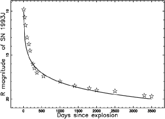
Figure 2: The $R$ LC of SN 1993J over 10 yr (empty stars) and theoretical curve as given by (32) (full line). In this case $t_{0}$ = 5 days, $d$ = 3.075, $k_{c}$ = 7.543 and $\alpha$ = 0.828. The data are extracted by the author from Figure 5 in Zhang et al. (2004).

The theoretical temporal evolution of the $H\alpha$ luminosity of SN 1993J as well the data are reported in Figure 3.

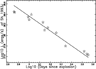
Figure 3: The Log-Log i-band (H$\alpha$ luminosity) LC of SN 1993J over 10 yr (empty stars) and theoretical curve as given by (41) (full line). In this case $t_{0}$ = 5 days, $d$ = 3.075, $\epsilon n_{1}=0.1$ and $\alpha$ = 0.828. The data are extracted by the author from Figure 7 in Zhang et al. (2004).

The $H\alpha$ luminosity which is derived from the $i-$band is also fitted by the model of Chevalier and Fransson (1994).

A second example is SN 2005cf (type Ia) which has been analyzed in Pastorello et al. (2007); Figure 4 and Figure 5 report the decay of the $V$ and $B$ magnitude of SN 2005cf as well our theoretical curve.

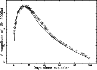
Figure 4: The $V$ LC of SN 2005cf (empty stars) and theoretical curve as given by the two phase model (46) (full line). The first phase is modeled by $t_{a}=5$ days and $k_{\nu}$ = 13.5 and the second phase by $t_{0}$ = 20.5 days, $d$ = 3.547, $k_{c}$ = 7.810 and $\alpha$ = 0.828. The data are the final S-corrected $V$ magnitudes reported in Table 6 of Pastorello et al. (200).

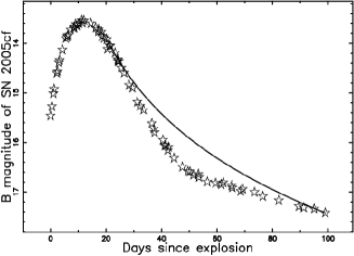
Figure 5: The $B$ LC of SN 2005cf (empty stars) and theoretical curve as given by (32) (full line). In this case $t_{0}$ = 20.5 days, $d$ = 3.83, $k_{c}$ = 7.286 and $\alpha$ = 0.828. The data are the final S-corrected $V$ magnitudes as reported in Table 6 of Pastorello et al. (2007).

The (B–V) color evolution of SN 2005cf is reported in Figure 6. Only the second phase is reported.

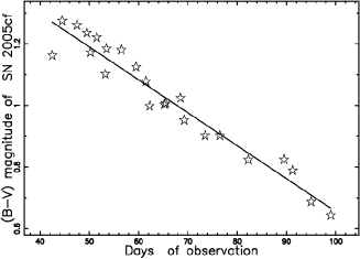
Figure 6: The (B–V) color evolution of SN 2005cf (empty stars) and the relative fitting straight line (full line). The time ranges from 40 days to 100 days.

A third example is the sample of 44 type Ia supernovae which have been observed in the UBVRI bands, see Jha et al. (2006). We selected SN 1999ac in the U band and Figure 7 reports the LC as well our fit.

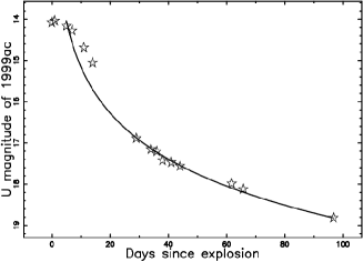
Figure 7: The $U$ LC of SN 1999ac (empty stars) and theoretical curve as given by (32) (full line). In this case $t_{0}$ = 5 days, $d$ = 3.17, $k_{c}$ = 11.44 and $\alpha$ = 0.828. The data are those reported at CDS.

A fourth example is SN 2001el (type Ia), which has been analyzed in Krisciunas et al. (2003). Figure 8 reports the decay of the $V$ magnitude of SN 2001el . A comparison should be made with Figure 4 of Kasen (2006) which uses the decay of ⁵⁶Ni.

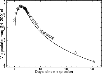
Figure 8: The $V$ LC of SN 2001el (empty stars) in absolute magnitude and theoretical curve as given by the two phase model (46) (full line). The first phase is modeled by $t_{a}=4$ days and $k_{\nu}=-18.64$, and the second phase by $t_{0}$ = 21 days, $d$ = 3.702, $k_{c}=-24.84$ and $\alpha$ = 0.828. The data are extracted from Table 3 of Krisciunas et al. (2003) and the adopted distance modulus is $\mu$ = 31.4 according to Kasen et al. (2006).

It is also interesting to plot the decay of the LC of SN 2001el , see Krisciunas et al. (2003), as given by two nuclear decay which, according to Equation (3), are straight lines, see Figure 9.

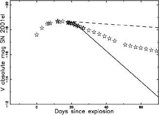
Figure 9: The $V$ LC of SN 2001el (empty stars) in absolute magnitude, theoretical curve as given by Equation (3) when the radioactive decay of the isotope ⁵⁶Ni ($\tau$ = 8.757 d or $T_{1/2}$ = 6.07 d) was considered (full line), and theoretical curve of the radioactive decay of the isotope ⁵⁶Co ($\tau$ = 111.47 d or $T_{1/2}$ = 77.27 d) was considered (dashed line).

5 Conclusions

The SN’s are classified as spherical SN, as an example SN 1993J , and as aspherical SN, see as an example Racusin et al. (2009) for SN  1987A . The theory here developed treats the spherical SN using classical dimensional arguments. The conversion of the flux of kinetic energy into luminosity after the maximum in the LC explains the curve of SNs in a direct form, see Equations (27) and (37) as well as in a logarithmic version, see Equation (32). The overall LC before and after the maximum can be built by introducing two different physical regimes, see Equation (46). The initial rise in intensity in the V-band is characterized by a typical time scale of $t_{a}\approx 5$ days and the decrease can be theoretically fitted for $t\approx 3500$ days. This large range in time is also the great advantage of our model: the existing nuclear models cover $\approx$ 100 days, see Figure 2 in Leibundgut and Suntzeff (2003). The standard approach of formula (2), which predicts a linear increase in the apparent magnitude with time, does not correspond to the observations because the observed and theoretical magnitudes scale as $m=a+b\,\ln(t)$ where $a$ and $b$ are two constants. As an example, Figure (9) reports two commonly accepted sources which are the radioactive isotopes ⁵⁶Co, see Georgii et al. (2000); Pluschke et al. (2001); Georgii et al. (2002), and ⁵⁶Ni, see Truran et al. (2012); Dessart et al. (2012): the radioactive fit is acceptable only for the first few days. The application of the new formulas to three SNs in different bands gives acceptable results. As an example, Figure 2 reports the LC in the R-band for SN 1993J and Figure 3 reports the LC for the $H\alpha$ of SN 1993J . An example of the two phase model as given by Equation (46) is reported in Figure (4) for SN 2005cf in the V-band. A careful analysis of the previous figures shows that the theoretical and observed curves present different concavities in the transition from small to large times. Similar results can be obtained assuming that all $\gamma$-rays produced by the decay of ⁵⁶Ni and ⁵⁶Co are converted into optical emission, see Figure 2 in Leibundgut and Suntzeff (2003). The observational fact that the initial velocity can be $\approx$ 30000 km s^-1 requires a relativistic treatment that is necessary for future progress. The analysis here performed treats the SN as a single object and therefore is not connected with various types of recent cosmologies, see Astier and Pain (2012); Chavanis (2013); ElNabulsi (2013).

We conclude with a list of not yet solved problems:

• The observational fact that the initial velocity can be $\approx 30000$ km s^-1 requires a relativistic treatment of the flux of kinetic energy that is left for future research;

• The connection between the cosmic ray production and the $\gamma$-rays in SNR, see Dermer and Powale (2013), requires an analysis of the temporal behavior of the magnetic field.

References

- Arnett (1980) Arnett, W. D. (1980), “Analytic solutions for light curves of supernovae of Type II,” ApJ , 237, 541–549.
- Arnett and Fu (1989) Arnett, W. D. and Fu, A. (1989), “The late behavior of supernova 1987A. I – The light curve. II – Gamma-ray transparency of the ejecta,” ApJ , 340, 396–425.
- Astier and Pain (2012) Astier, P. and Pain, R. (2012), “Observational evidence of the accelerated expansion of the universe,” Comptes Rendus Physique, 13, 521–538.
- Bowers and Deeming (1984) Bowers, R. L. and Deeming, T. (1984), Astrophysics. I and II, Boston: Jones and Bartlett .
- Chavanis (2013) Chavanis, P.-H. (2013), “A cosmological model describing the early inflation, the intermediate decelerating expansion, and the late accelerating expansion by a quadratic equation of state,” ArXiv e-prints.
- Chevalier (1982a) Chevalier, R. A. (1982a), “Self-similar solutions for the interaction of stellar ejecta with an external medium,” ApJ , 258, 790–797.
- Chevalier (1982b) — (1982b), “The radio and X-ray emission from type II supernovae,” ApJ , 259, 302–310.
- Chevalier and Fransson (1994) Chevalier, R. A. and Fransson, C. (1994), “Emission from circumstellar interaction in normal Type II supernovae,” ApJ , 420, 268–285.
- De Young (2002) De Young, D. S. (2002), The Physics of Extragalactic Radio Sources, Chicago: University of Chicago Press.
- Dermer and Powale (2013) Dermer, C. D. and Powale, G. (2013), “Gamma rays from cosmic rays in supernova remnants,” A&A , 553, A34.
- Dessart et al. (2012) Dessart, L., Hillier, D. J., Waldman, R., Livne, E., and Blondin, S. (2012), “Superluminous supernovae: 56Ni power versus magnetar radiation,” MNRAS , 426, L76–L80.
- Dyson, J. E. and Williams, D. A. (1997) Dyson, J. E. and Williams, D. A. (1997), The Physics of the Interstellar Medium, Bristol: Institute of Physics Publishing.
- ElNabulsi (2013) ElNabulsi, R. A. (2013), “Some late-time cosmological aspects of a Gauss–Bonnet gravity with nonminimal coupling à la Brans–Dicke: Solutions and perspectives,” Canadian Journal of Physics, 91, 300–321.
- Eriksen et al. (2009) Eriksen, K. A., Arnett, D., McCarthy, D. W., and Young, P. (2009), “The reddening toward Cassiopeia A’s supernova: Constraining the 56Ni yield,” ApJ , 697, 29–36.
- Falk and Arnett (1973) Falk, S. W. and Arnett, W. D. (1973), “A theoretical model for type II supernovae,” ApJ , 180, L65.
- Fan et al. (2010) Fan, Z., Liu, S., and Fryer, C. L. (2010), “Stochastic electron acceleration in the TeV supernova remnant RX J1713.7-3946: The high-energy cut-off,” MNRAS , 406, 1337–1349.
- Freedman et al. (1994) Freedman, W. L., Hughes, S. M., Madore, B. F., Mould, J. R., and Lee, M. G. (1994), “The Hubble Space Telescope Extragalactic Distance Scale Key Project. 1: The discovery of Cepheids and a new distance to M81,” ApJ , 427, 628–655.
- Georgii et al. (2000) Georgii, R., Pluschke, S., Diehl, R., Collmar, W., Lichti, G. G., Schonfelder, V., Bloemen, H., Knodlseder, J., McConnell, M., Ryan, J., and Bennett, K. (2000), “COMPTEL upper limits for the 56Co -rays from SN1998bu,” in American Institute of Physics Conference Series, eds. McConnell, M. L. and Ryan, J. M., vol. 510 of American Institute of Physics Conference Series, pp. 49–53.
- Georgii et al. (2002) Georgii, R., Pluschke, S., Diehl, R., Lichti, G. G., Schonfelder, V., Bloemen, H., Hermsen, W., Ryan, J., and Bennett, K. (2002), “COMPTEL upper limits for the 56Co gamma-ray emission from SN1998bu,” A&A , 394, 517–523.
- Grasberg et al. (1971) Grasberg, E. K., Imshenik, V. S., and Nadyozhin, D. K. (1971), “On the theory of the light curves of supernovate (in Russian),” Astrophysics and Space Science , 10, 3.
- Jack et al. (2011) Jack, D., Hauschildt, P. H., and Baron, E. (2011), “Theoretical light curves of type Ia supernovae,” A&A , 528, A141+.
- Jha et al. (2006) Jha, S., Kirshner, R. P., Challis, P., Garnavich, P. M., and Matheson, T. (2006), “UBVRI light curves of 44 type Ia supernovae,” AJ , 131, 527–554.
- Kasen (2006) Kasen, D. (2006), “Secondary maximum in the near-infrared light curves of type Ia supernovae,” ApJ , 649, 939–953.
- Kasen and Woosley (2009) Kasen, D. and Woosley, S. E. (2009), “Type II supernovae: Model light curves and standard candle relationships,” ApJ , 703, 2205–2216.
- Katsuda et al. (2010) Katsuda, S., Petre, R., Mori, K., Reynolds, S. P., Long, K. S., Winkler, P. F., and Tsunemi, H. (2010), “Steady X-ray synchrotron emission in the northeastern limb of SN 1006,” ApJ , 723, 383–392.
- Krisciunas et al. (2003) Krisciunas, K., Suntzeff, N. B., Candia, P., Arenas, J., Espinoza, J., Gonzalez, D., Gonzalez, S., Hoflich, P. A., Landolt, A. U., Phillips, M. M., and Pizarro, S. (2003), “Optical and infrared photometry of the nearby type Ia supernova 2001el,” AJ , 125, 166–180.
- Lang (1999) Lang, K. R. (1999), Astrophysical Formulae. (Third Edition), New York: Springer.
- Leibundgut and Suntzeff (2003) Leibundgut, B. and Suntzeff, N. B. (2003), “Optical light curves of supernovae,” in Supernovae and Gamma-Ray Bursters, ed. Weiler, K., vol. 598 of Lecture Notes in Physics, Berlin: Springer-Verlag, pp. 77–90.
- Marcaide et al. (2009) Marcaide, J. M., Martí-Vidal, I., Alberdi, A., and Pérez-Torres, M. A. (2009), “A decade of SN 1993J: Discovery of radio wavelength effects in the expansion rate,” A&A , 505, 927–945.
- Martí-Vidal et al. (2011) Martí-Vidal, I., Marcaide, J. M., Alberdi, A., Guirado, J. C., Pérez-Torres, M. A., and Ros, E. (2011), “Radio emission of SN1993J: The complete picture. II. Simultaneous fit of expansion and radio light curves,” A&A , 526, A143+.
- McCray (1987) McCray, R. A. (1987), “Coronal interstellar gas and supernova remnants,” in Spectroscopy of Astrophysical Plasmas, ed. A. Dalgarno & D. Layzer, pp. 255–278.
- Padmanabhan (2001) Padmanabhan, P. (2001), Theoretical Astrophysics. Vol. II: Stars and Stellar Systems, Cambridge University Press.
- Pastorello et al. (2007) Pastorello, A., Taubenberger, S., et al. (2007), “ESC observations of SN 2005cf—I. Photometric evolution of a normal type Ia supernova,” MNRAS , 376, 1301–1316.
- Petruk and Beshlei (2007) Petruk, O. and Beshlei, V. (2007), “Synchrotron and thermal X-ray emission from supernova remnants. Low radiation losses of electrons,” Kinematics and Physics of Celestial Bodies, 23, 16–27.
- Pluschke et al. (2001) Pluschke, S., Georgii, R., Diehl, R., Collmar, W., Lichti, G. G., Schonfelder, V., Bloemen, H., Hermsen, W., Bennett, K., McConnell, M., and Ryan, J. (2001), “56Co -rays from SN1998bu: COMPTEL upper limits,” in Exploring the Gamma-Ray Universe, eds. Gimenez, A., Reglero, V., and Winkler, C., vol. 459 of ESA Special Publication, pp. 87–90.
- Press et al. (1992) Press, W. H., Teukolsky, S. A., Vetterling, W. T., and Flannery, B. P. (1992), Numerical Recipes in FORTRAN. The Art of Scientific Computing, Cambridge University Press.
- Racusin et al. (2009) Racusin, J. L., Park, S., Zhekov, S., Burrows, D. N., Garmire, G. P., and McCray, R. (2009), “X-ray evolution of SNR 1987A: The radial expansion,” ApJ , 703, 1752–1759.
- Reynolds (2011) Reynolds, S. P. (2011), “Particle acceleration in supernova-remnant shocks,” Astrophysics and Space Science , 336, 257–262.
- Ripero et al. (1993) Ripero, J., Garcia, F., Rodriguez, D., Pujol, P., Filippenko, A. V., Treffers, R. R., Paik, Y., Davis, M., Schlegel, D., Hartwick, F. D. A., Balam, D. D., Zurek, D., Robb, R. M., Garnavich, P., and Hong, B. A. (1993), “Supernova 1993J in NGC 3031,” IAU circ. , 5731, 1.
- Rybicki and Lightman (1991) Rybicki, G. and Lightman, A. (1991), Radiative Processes in Astrophysics, New York: Wiley.
- Schure et al. (2010) Schure, K. M., Achterberg, A., Keppens, R., and Vink, J. (2010), “Time-dependent particle acceleration in supernova remnants in different environments,” MNRAS , 406, 2633–2649.
- Sedov (1944) Sedov, L. I. (1944), “Decay of isotropic turbulent motions of an incompressible fluid,” Dokl. Akad. Nauk. SSSR, 42, 116.
- Sedov (1959) — (1959), Similarity and Dimensional Methods in Mechanics, New York: Academic Press.
- Taylor (1950a) Taylor, G. (1950a), “The formation of a blast wave by a very intense explosion. I. Theoretical discussion,” Royal Society of London Proceedings Series A, 201, 159–174.
- Taylor (1950b) — (1950b), “The formation of a blast wave by a very intense explosion. II. The atomic explosion of 1945,” Royal Society of London Proceedings Series A, 201, 175–186.
- Truran et al. (2012) Truran, J. W., Glasner, A. S., and Kim, Y. (2012), “56Ni, explosive nucleosynthesis, and SNe Ia diversity,” Journal of Physics Conference Series, 337, 012040.
- van Hise (1974) van Hise, J. R. (1974), “Light-decay curve of the supernova in IC 4182,” ApJ , 192, 657–659.
- Zaninetti (2009) Zaninetti, L. (2009), “Scaling for the intensity of radiation in spherical and aspherical planetary nebulae,” MNRAS , 395, 667–691.
- Zaninetti (2010) — (2010), “A law of motion for spherical shells in special relativity,” Advanced Studies in Theoretical Physics, 4, 525–534.
- Zaninetti (2011) — (2011), “Time-dependent models for a decade of SN 1993J,” Astrophysics and Space Science , 333, 99–113.
- Zhang et al. (2004) Zhang, T., Wang, X., Zhou, X., Li, W., Ma, J., Jiang, Z., and Li, Z. (2004), “Optical photometry of SN 1993J: 1995 to 2003,” AJ , 128, 1857–1867.