Low-temperature data for carbon dioxide

Abstract

We investigate the empirical data for the vapor pressure (154$\leq$$T$$\leq$196 K) and heat capacity (15.52$\leq$$T$$\leq$189.78 K) of the solid carbon dioxide. The approach is both theoretical and numerical, using a computer algebra system (CAS). From the latter point of view, we have adopted a cubic piecewise polynomial representation for the heat capacity and reached an excellent agreement between the available empirical data and the evaluated one. Furthermore, we have obtained values for the vapor pressure and heat of sublimation at temperatures below 195 right down to 0 K. The key prerequisites are the: 1) Determination of the heat of sublimation of 26250 J$\cdot$mol^-1 at vanishing temperature and 2) Elaboration of a ‘linearized’ vapor pressure equation that includes all the relevant properties of the gaseous and solid phases. It is shown that: 1) The empirical vapor pressure equation derived by Giauque & Egan remains valid below the assumed lower limit of 154 K (similar argument holds for Antoine’s equation), 2) The heat of sublimation reaches its maximum value of 27211 J$\cdot$mol^-1 at 58.829 K and 3) The vapor behaves as a (polyatomic) ideal gas for temperatures below 150 K.

I Introduction

Because of the intensive use of carbon dioxide in industry and research carbon , it has become necessary to determine its thermodynamic, physical and chemical properties on an extended range of temperatures. Significant effort has been deployed to build up a database through observations and theoretical calculations Meyers ; Giauque ; d2 ; Suzuki ; Schnepp ; Ron ; G ; Gray ; nist ; tool ; Jr ; IoP . From the former point of view, we mention the case of the accurate measurements due to Giauque & Egan Giauque and from the latter point of view, the derivation based on the classical version of the theory of lattice dynamics, which predicts the heat capacity of carbon dioxide in the range of temperatures 15$<$$T$$<$50 K Suzuki , is in a very good agreement with that obtained through observations Giauque .

However, such a good agreement is still out of reach for some other properties of carbon dioxide due to difficulties from both experimental and theoretical points of view. For instance, the empirical determination of the latent heat of sublimation at low temperatures remains a major obstacle because of the difficulty in eliminating the superheating of the gas Giauque . Similarly, by way of example, the lagrangian classical treatment of the two-dimensional rigid rotor is intractable and the theoretical determination of the heat capacity, mentioned above, had been made possible at only sufficiently low temperatures ($T$$<$50 K) when the harmonic approximation is valid Schnepp . With that said, much work has to be done in order to determine further properties of carbon dioxide particularly at low temperatures, such properties are still missing in the best compendia.

We will exploit the data available in Giauque , which we refer to as G&E, and show that it is possible to evaluate the heat of sublimation $L$ and vapor pressure $p$ at temperatures 5$\leq$$T$$\leq$195 K. A key prerequisite is the determination of the heat of sublimation at $T$=0 K ($L(0)$=$\epsilon_{0}$). Stull calculated an average value of $L$ by the method of least squares using the vapor pressure data measured by different workers d2 and obtained a value of 26.3 kJ$\cdot$mol^-1 (=6286 cal$\cdot$mol^-1) for 139$\leq$$T$$\leq$195 K nist . However, the literature citations listed in d2 show that Stull did not extract data from G&E, which is even more accurate and includes data concerning the heat capacity of the solid carbon dioxide and other data that could be used to obtain $L$ at different temperatures. By contrast, G&E have evaluated $L$ at 194.67 K using partly their measured data and available data for $L$ at lower temperatures Meyers . They evaluated the integral of the heat capacity of the solid (change in the enthalpy) graphically from a smooth curve through their measured data and obtained a value for $L$ that is merely 10 cal$\cdot$mol^-1 higher than their measured value $L_{\rm{meas}}(194.67)$=6030$\pm$5 cal$\cdot$mol^-1 (25230$\pm$21 J$\cdot$mol^-1). They also evaluated the entropies of the gas and solid at 194.67 K and reached an excellent agreement between experimental data and statistics (the experimental & spectroscopic values of the entropy of the gas $s_{g}$ they obtained were 47.59 & 47.55 cal$\cdot$K^-1$\cdot$mol^-1, respectively, constituting a proof of the third law d3 ). However, this cumbersome procedure had prevented them from carrying out a systematic evaluation of the latent heat and entropy at temperatures covering the range of their measured data. Furthermore, this procedure (the graphical evaluation) adds a human error, which is an unknown factor.

In this paper we will carry out a systematic evaluation of the fore-mentioned physical quantities on a more extended range of temperatures than that of G&E using 1) a computer algebra system (CAS), which eliminates the human error and allows an excellent adjustment of the parameters in order to achieve a better accuracy, as well as 2) an established formula for the vapor pressure. It will be shown below that our reevaluated value of $L(194.67)$ is 6030.4 cal$\cdot$mol^-1 (25231 J$\cdot$mol^-1). The data for the relevant quantities will be tabulated at temperatures incremented by 5 K and plotted. Moreover, the generating codes will be provided, which allow the evaluation of any quantity at any given temperature within minutes of time. In this work, we will be relying on measured data by different workers and on some empirical formulas derived by graphical interpolation. Since some of these data are provided without accuracy and some other lack accuracy due to personal error, it will be difficult to assign accuracy to our results, as is the case in most compendia. Some values of $p$ (in Torr) will be given with one significant digit while other values with 2 or 3 significant digits. The values of $L$ (of the order of 26000 J$\cdot$mol^-1) will be given with five digits without decimals, assuming an error not higher than 0.35%. The accuracy of the results for $p$ and $L$ can be read by comparing with the available measured data.

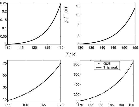
Figure 1: The vapor pressure vs. the temperature. Solid line: This work (TW) plotted for 110$\leq$$T$$\leq$195, dotted line: G&E plotted for 155$\leq$$T$$\leq$196.

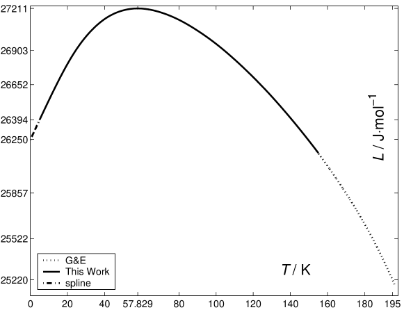
Figure 2: The heat of sublimation vs. the temperature. Solid line: This work (TW) plotted using the derived Eq. (12), dotted line: plotted using the same equation with $p_{\,\rm G\&E}\,$, dash-dot line: arc of the spline through the data ($T,L_{\,\rm TW}$) & $T$=5$n$ K (0$\leq$$n$$\leq$31, positive integer) shown in Table II. This arc extrapolates the solid line to temperatures below 5 K.

II Results and Discussions

Heat of sublimation at $\boldsymbol{T=0}$.

Throughout this paper, we use the units and symbols recommended by the International Union of Pure and Applied Chemistry (IUPAC) IUPAC . The energy is given in J and in cal = 4.184 J, the pressure in Torr, and the temperature in K. Since the original data were given in calories, we perform our evaluations in this unit, taking $R$=1.98724 cal$\cdot$K^-1$\cdot$mol^-1, then convert the results to joules.

The G&E heat capacity measurements, shown in the codes (appendix), extend from 15.52 to 189.78 K. On such a large interval there is no best equation that will represent the data d3 . G&E worked on a smooth curve through the data but did not describe it. In order to represent the data, the alternative is to subdivide the interval into sufficiently small intervals and represent the data by a polynomial on each sub-interval in such a way that the polynomial pieces blend smoothly making a spline mat .

MATLAB provides spline curve via the command spline(x,y) (see Appendix Section). It returns the piecewise polynomial form of the cubic spline interpolant with the not-a-knot end conditions, having two continuous derivatives and breaks at all interior data sites except for the leftmost and the rightmost one. The values of the spline at the breaks spline(x,y,x(i)) coincide with the data values y(i). Cubic splines are more attractive for interpolation purposes than higher-order polynomials mat .

We will deal with molar physical quantities labeled by the subscripts $s$ & $g$ to differentiate between the solid and gaseous phases. We denote by $L$ the latent heat of sublimation and by $u_{i}$, $a_{i}$, $\mu_{i}$, $v_{i}$, $h_{i}$, $s_{i}$ ($i$=$s,g$), the internal energy, free energy, chemical potential, volume, enthalpy, entropy, respectively. We take the zero of rotational energy to be that of the $J$=0 state and the zero of vibrational energy to be that of the ground state, meaning that a molecule at rest in the gas has an energy of zero at vanishing temperature ($u_{g}(0)$=0). Let $\epsilon_{0}$ be the heat of sublimation at $T$=0 which is, according to our energy convention, the binding energy of the particles of the solid ($u_{s}(0)$=$a_{s}(0)$=${h}_{s}(0)$=$\mu_{s}(0)$=$-\epsilon_{0}$$<$0).

The excellent agreement between the experimental & spectroscopic values of $s_{g}$ at 194.67 K is due to G&E accurate measurements and to the success of Debye’s theory at low temperatures. G&E used Debye’s formula to evaluate $s_{s}$ for 0$\leq$$T$$\leq$15 K. However, they did not explain their choice for Debye’s temperature $\theta_{D}\,$. In this work, the energy and entropy of the solid for temperatures below 15.52 K are extrapolated by substitution of the Debye heat capacity formula. Moreover, we will rely on Suzuki & Schnepp’s assertion that the molar heat capacities of the solid carbon dioxide ($c_{v}$ & $c_{p}$) are equal within an error of 10^-5 per cent for such small temperatures Suzuki . Finally, we fix $\theta_{D}$ by equating the heat capacity due to Debye with that measured by G&E at 15.52 K (0.606 cal$\cdot$K^-1$\cdot$mol^-1). Solving the equation using a CAS we find $\theta_{D}$=139.59 K.

The MATLAB codes provided in the appendix are split into three parts. In Part (I), cd represents the Debye heat capacity. The vectors t & cp show the temperature data sites used by G&E (15.52$\mapsto$189.78 K) and the corresponding measured heat capacities (0.606$\mapsto$13.05 cal$\cdot$K^-1$\cdot$mol^-1), respectively. These G&E data sites are extended by the temperature vector u and the corresponding Debye heat capacity vector v, respectively. The last two lines evaluate, at the temperature vector Tn, the spline through the extended data sites (t, cp), the integrals $\int_{0}^{T}c_{p}\,{\rm d}T^{\prime}$=$h_{s}(T)+\epsilon_{0}$=$\Delta h_{s}(T)$ (vector I) and $\int_{0}^{T}(c_{p}/T^{\prime})\,{\rm d}T^{\prime}$=$s_{s}(T)$ (vector J), with $T\in$ Tn.

The heat of sublimation $\epsilon_{0}$ is determined upon solving the equation $\mu_{g}$=$\mu_{s}$ at any given temperature for which the measured $L$ is known. The lead we had followed seeking for higher accuracy led us to select the value of $L$=$6190$ cal$\cdot$mol^-1 at $170$ K (Meyers, , Eucken & Donath) & Giauque . We find $\epsilon_{0}$=$6273.4$ cal$\cdot$mol^-1 and the calculation is shown below.

With $\mu_{g}$=$a_{g}+p\,v_{g}$ & $\mu_{s}$=${h}_{s}-T\,s_{s}\,$, the equation $\mu_{g}$=$\mu_{s}$ reduces to $\epsilon_{0}$=$\Delta h_{s}-T\,s_{s}-a_{g}-p\,v_{g}\,$. Upon solving the Clapeyron equation for $p\,v_{g}$ we obtain $p\,v_{g}$=$[L/(T\,{\rm d}\ln p/{\rm d}T)]+p\,v_{s}$, and finally

$$\epsilon_{0}=\Delta h_{s}-T\,s_{s}-a_{g}-\frac{L}{T({\rm d}\ln p/{\rm d}T)}-p\,v_{s}\,.$$ (1)

We will make use of the G&E empirical equation to evaluate $p$ & ${\rm d}\ln p/{\rm d}T$ at 170 K

$$p_{\,\rm G\&E}({\rm Torr})=10\,{\rm exp}[(a_{1}/T)+b_{1}+c_{1}\,T+d_{1}\,T^{2}]\quad(154\leq T\leq 196\,{\rm K}),$$ (2)

($a_{1}$=$-$1354.210$\times$$\ln 10$, $b_{1}$=8.69903$\times$$\ln 10$, $c_{1}$=0.001588$\times$$\ln 10$, $d_{1}$=$-$4.5107$\times$$10^{-6}$$\times$$\ln 10$), and obtain $p(170)$=74.59 Torr. Since $v_{s}$=25.55 cm³$\cdot$mol^-1 Suzuki , the last term $p\,v_{s}$=0.06 cal$\cdot$mol^-1 is neglected. The term including $L$ equals 6190/(170$\times$0.108021)=337.08 cal$\cdot$mol^-1, and $\Delta h_{s}(170)\;\&\;s_{s}(170)$ are the 85000^th components of the vectors I & J: $\Delta h_{s}(170)-170\times s_{s}(170)$=I(85000)-170*J(85000)=$-$1227.8 cal$\cdot$mol^-1.

Now, we make our first hypothesis concerning the vapor. We assume the validity of the first order virial expansion neglecting thus the next terms, and this has always been the case for carbon dioxide Giauque at such low temperatures. We have then

$$p\,v_{g}=R\,T+B(T)\,p\,,$$ (3)

thereby we can show that the term $a_{g}$ in (1) is the free energy of an ideal gas evaluated at the point $(T,p)$=$(170\,{\rm K},74.59\,{\rm Torr})\,$. For the molecule of CO₂ we have $a_{g}$=$a_{\rm t}+a_{\rm r}+a_{\rm v}$, which is the sum of the translational, rotational and four vibrational contributions $a_{\rm v}$=$2\,a_{\rm v1}+a_{\rm v2}+a_{\rm v3}$ MQ ; HG . With our choice of the origin of the energy, these contributions write

$$a_{\rm t}=-R\,T\,\ln(\mathcal{C}\,{\rm e}\,T^{5/2}/p)\,;$$

   ,

(4)

with ${\mathcal{C}}$=7.575455$\times 10^{5}$ in SI units (=$(2\,\pi\,m/h^{2})^{3/2}\,k^{5/2}$) and $\theta_{\rm r}$=0.561, $\theta_{\rm v1}$=954, $\theta_{\rm v2}$=1890, $\theta_{\rm v3}$=3360 K. We have then $a_{g}(170)$=$-$7838.2 cal$\cdot$mol^-1 leading with the previously evaluated terms to $\epsilon_{0}$=6273.4 cal$\cdot$mol^-1.

Vapor pressure.

From now on we will assume $\epsilon_{0}$=6274 cal$\cdot$mol^-1 (26250 J$\cdot$mol^-1). Upon substituting (3) & (4) into $\epsilon_{0}$=$\Delta h_{s}-T\,s_{s}-a_{g}-p\,v_{g}$ ($\mu_{g}$=$\mu_{s}$) and rearranging the terms we obtain

$$p={\mathcal{C}}\,T^{5/2}Z_{\rm r}\,Z_{\rm v}\,{\rm exp}\{[\Delta h_{s}-T\,s_{s}-\epsilon_{0}-B(T)\,p]/RT\}\,,$$ (5)

where $Z_{\rm v}$=$Z_{\rm v1}^{2}Z_{\rm v2}Z_{\rm v3}\,$, $Z_{\rm vi}$=$1/[1-{\rm exp}(-\theta_{\rm vi}/T)]\,({\rm i}$=$1-3)$, and $Z_{\rm r}$=$[T+\theta_{\rm r}/3]/(2\,\theta_{\rm r})\,$. Assuming that $B(T)$ follows Berthelot’s equation Giauque ; d3

$$B(T)\,p=R\,\ell_{1}[1-(\ell_{2}/T^{2})]\,p({\rm Torr})$$ (6)

(where $\ell_{2}$=6$\times$304.1² K² and, in order to express $B(T)\,p$ in cal$\cdot$mol^-1, we take $\ell_{1}$=9$\times$304.1/(128$\times$72.8$\times$760) K/Torr), we have solved numerically both equation (5) and its linearized form and the results coincide up to an insignificant error. Upon substituting exp$[-B(T)p/RT]$=$1-B(T)p/RT$ into (5), the linearized equation yields

$$p_{\,\rm TW}({\rm Torr})=\frac{p_{\,\rm ideal}}{\{1+\ell_{1}[1-(\ell_{2}/T^{2})]p_{\,\rm ideal}/T\}}\quad(T\geq 5\,{\rm K})\,,$$ (7)

where $p_{\,\rm ideal}$ (in Torr) is the corresponding pressure for an ideal gas

$$p_{\,\rm ideal}({\rm Torr})=(760/101325)\,{\mathcal{C}}\,T^{5/2}Z_{\rm r}\,Z_{\rm v}\,{\rm exp}\{[\Delta h_{s}-T\,s_{s}-\epsilon_{0}]/RT\}\,.$$ (8)

Table II & FIG. 1 compare values of the vapor pressure derived in this work (TW) with those of G&E (Eqs. (7) & (2)). We have evaluated (2) at temperatures below the left-end point 154 K, as shown in Table II, and the formula remains applicable, however, for temperatures above 110 K; below this temperature, equation (2) diverges from (7). The third column (A) of Table II shows values of the vapor pressure evaluated using Antoine’s equation d3 . The constants $A_{1}$=6.81228, $B_{1}$=1301.679 & $C_{1}$=$-$3.494 of Antoine’s equation have been evaluated by the National Institute of Standards and Technology (NIST) nist from G&E data. The equation writes

$$p_{\,\rm A}({\rm Torr})=(760/1.01325){\rm exp}\{\bar{A_{1}}-[\bar{B_{1}}/(A_{1}T+C_{1})]\}\quad(154.26\leq T\leq 195.89\,{\rm K}),$$ (9)

where $\bar{A_{1}}$=$A_{1}\ln 10$, $\bar{B_{1}}$=$B_{1}\ln 10$.

Table 1: Vapor pressure data. The values of the pressure shown in italics are evaluated at temperatures beyond the assumed range of validity of the corresponding formula. The table compares our results TW: This work (Eq. (7)) with those of G&E (Eq. (2)) Giauque and Antoine’s equation (Eq. (9)) nist . Nomenclature: NA=Not Applicable. Conventions: 1) E–n=$10^{-n}\,$; 2) a letter C shown on the right of a $p$-value indicates that a small correction for gas imperfection has been added; if, otherwise, the values of $p$ with and without correction are equal ($p$=$p_{\,\rm ideal}$). Since the G&E and A data are empirical, a letter C has been added to all of them including those values evaluated beyond the assumed range of validity.

$T$/K	$p_{\,\rm TW}$/Torr	$p_{\,\rm G\&E}$/Torr	$p_{\,\rm A}$/Torr
65	3.4E–12	NA	3.3E–12(C)
70	1.2E–10	NA	1.3E–10(C)
75	2.8E–9	NA	3.0E–9(C)
80	4.2E–8	NA	4.7E–8(C)
85	4.7E–7	NA	5.2E–7(C)
90	3.9E–6	NA	4.3E–6(C)
95	2.6E–5	NA	2.8E–5(C)
100	1.4E–4	NA	1.5E–4(C)
105	6.8E–4	NA	7.3E–4(C)
110	0.003	0.003(C)	0.003(C)
115	0.01	0.01(C)	0.01(C)
120	0.03	0.03(C)	0.03(C)
125	0.09	0.09(C)	0.09(C)
130	0.2	0.2(C)	0.2(C)
135	0.6	0.6(C)	0.6(C)
140	1.4	1.4(C)	1.4(C)
145	3.1	3.1(C)	3.1(C)
150	6.4	6.4(C)	6.3(C)
155	12.5	12.6(C)	12.5(C)
160	23.6	23.6(C)	23.5(C)
165	42.8(C)	42.7(C)	42.4(C)
170	74.6(C)	74.6(C)	74.1(C)
175	126(C)	126(C)	125(C)
180	206(C)	207(C)	205(C)
185	329(C)	330(C)	328(C)
190	511(C)	513(C)	511(C)
195	776(C)	781(C)	777(C)

From Table II we establish the following results. Equations (2) & (9) are still valid beyond their assumed ranges of validity; the ranges are now extended right down below their left-end points to include temperatures above 110 and 65 K, respectively. Moreover, the vapor behaves as a polyatomic ideal gas for temperatures below 155 K.

An instance of calculation is provided in the codes provided in Part(II) of the appendix, which show the evaluation of the ideal-gas pressure equation (8) & the real-gas pressure equation (7) at 160, 180 & 194.67 K. The evaluated pressures are represented by the 3-vectors PI and PTW, respectively.

Heat of sublimation.

Combining different thermodynamic entities we establish the equation

$$L(T)=\epsilon_{0}-\Delta h_{s}(T)+h_{g}(T)+[B(T)-(T\,{\rm d}B/{\rm d}T)]\,p(T)\,,$$ (10)

where the last two terms add a correction for gas imperfection, $p(T)$ is the vapor pressure and $h_{g}$ is the ideal-gas enthalpy given by $h_{g}$=$R\,[(7T/2)$$-$$(\theta_{\rm r}/3)]$$-$$T^{2}[{\rm d}(a_{\rm v}/T)/{\rm d}T]$ (Eq. (4)).

Looking for extreme values we can first ignore the correction for gas imperfection then justify it later. We have solved graphically the equation ${\rm d}L/{\rm d}T$=0 ($c_{p\,s}$=$c_{p\,g}$) and obtained the values 57.829 K for $T$ & 6503.58 cal$\cdot$mol^-1 for $L$ as shown in FIG. 2. We will assume $L_{\rm max}$=6503.6 cal$\cdot$mol^-1 (27211 J$\cdot$mol^-1). Tables II & II, however, show that at 57.829 K the vapor behaves as an ideal gas, and this justifies the omission of the correction terms in ${\rm d}L/{\rm d}T$=0.

Substituting (6) into (10), this latter splits into two equations whether we evaluate the vapor pressure using (2) or (7)

$$L_{\,\rm G\&E} = \epsilon_{0}-\Delta h_{s}+h_{g}+R\,\ell_{1}[1-(3\ell_{2}/T^{2})]\,p_{\,\rm G\&E}\quad(154\leq T\leq 196\,{\rm K}),$$ (11)

$$L_{\,\rm TW} = \epsilon_{0}-\Delta h_{s}+h_{g}+R\,\ell_{1}[1-(3\ell_{2}/T^{2})]\,p_{\,\rm TW}\quad(T\geq 5{\rm K})\,.$$ (12)

Equations (11) & (12) are plotted in FIG. 2. In the codes provided in Part(III) of the appendix, we evaluate the r.h.s of (12) at 160, 180 & 194.67 K (3-vector LTW). The value of the latent heat obtained at 194.67 K is 6030.4 cal$\cdot$mol^-1 (25231 J$\cdot$mol^-1) or 6030.6 cal$\cdot$mol^-1 (25232 J$\cdot$mol^-1) whether we calculate the r.h.s of (12) or (11).

Table 2: Heat of sublimation data. The values of the latent heat shown in italics are evaluated at temperatures beyond the assumed range of validity of the corresponding formula. The table compares our results TW: This work (Eq. (12)) with those derived from Eq. (11) using G&E pressure equation. Nomenclature: NA=Not Applicable. Convention: a letter C shown on the right of a $L$-value indicates that a small correction for gas imperfection has been added; if, otherwise, the values of $L$ with and without correction are equal.

$T$/K	$L_{\,\rm TW}$/J$\cdot$mol-1	$L_{\,\rm G\&E}$/J$\cdot$mol-1
0	26250	NA
5	26394	NA
10	26538	NA
15	26676	NA
20	26804	NA
25	26914	NA
30	27005	NA
35	27077	NA
40	27133	NA
45	27172	NA
50	27197	NA
55	27209	NA
60	27210	NA
65	27201	NA
70	27183	NA
75	27158	NA
80	27128	NA
85	27091	NA
90	27048	NA
95	27002	NA
100	26951	NA
105	26896	NA
110	26836	26836
115	26773	26773
120	26707	26707
125	26637	26637
130	26565	26565
135	26488	26488
140	26408	26408
145	26325	26325
150	26239(C)	26239(C)
155	26149(C)	26149(C)
160	26055(C)	26055(C)
165	25958(C)	25958(C)
170	25855(C)	25855(C)
175	25745(C)	25745(C)
180	25629(C)	25629(C)
185	25504(C)	25504(C)
190	25368(C)	25368(C)
195	25221(C)	25220(C)

In concluding, it was of interest to further compare our results for the pressure with those used by Stull d2 that, as already stated, are less accurate than G&E values. At temperatures 138.8, 148.7, 153.6, 158.7 K, we read from d2 the values 1, 5, 10, 20 Torr for the pressure, while our evaluated values (Eq. (7)) are 1.16, 5.30, 10.42, 20.12 Torr, respectively. Finally, values of the entropy of the solid at the tabulated temperatures $T$=5$j$ K (1$\leq$$j$$\leq$39, positive integer) form a sub-vector of J and are obtainable upon executing the codes q=2500:2500:97500; J(q). For instance, $s_{s}(160)$=J(80000)=14.07, $s_{s}(180)$=J(90000)=15.50 and $s_{s}(194.67)$=J(97335)=16.52 cal$\cdot$K^-1$\cdot$mol^-1 (58.87, 64.85 & 69.12 J$\cdot$K^-1$\cdot$mol^-1, respectively).

III Methods

Concerning the numerical approach, given the accurate data for the heat capacity at constant pressure of carbon dioxide and some available data for the heat of sublimation, we employed the method of splines to generate and evaluate a smooth curve representing the heat capacity data. Dealing with a large number of data sites, we preferred to use cubic splines, which are more attractive for interpolation purposes than higher-order polynomials mat . Once the curve set, we proceeded to the evaluation of the change of the enthalpy and entropy of the solid. The evaluation of the relevant physical quantities concerning the vapor was rather straightforward using almost fresh formulas from the thermodynamic literature MQ ; HG . We used MATLAB to execute the task and the calculated entities were used in subsequent vapor pressure and heat of sublimation evaluations.

Now, concerning the theoretical approach, we mainly derived a formula for the vapor pressure including a correction for gas imperfection and effects for internal structure, as well as a formula for the heat of sublimation with same purposes.

IV acknowledgments

The author acknowledges comments and suggestions by an anonymous referee, which helped to improve the manuscript.

Appendix
This section is devoted to provide the main MATLAB codes, as a part of the numerical method, leading to the results shown in this paper.

Part(I)
Part(I) shows the data sites used by G&E (15.52$\mapsto$189.78 K) & (0.606$\mapsto$13.05 cal$\cdot$K^-1$\cdot$mol^-1). We evaluate the spline through the extended data sites (t, cp), the integrals $\int_{0}^{T}c_{p}\,{\rm d}T^{\prime}$=$h_{s}(T)+\epsilon_{0}$=$\Delta h_{s}(T)$ (vector I) and $\int_{0}^{T}(c_{p}/T^{\prime})\,{\rm d}T^{\prime}$=$s_{s}(T)$ (vector J), with $T\in$ Tn.

syms x z real;
f=(12/(x^3))*int((z^3)/(exp(z)-1),z,0,x);
g=(3*x)/(exp(x)-1); A=f-g; cd=3*1.98724*A;
u=0.01:0.01:15.25; xn=139.59./u;
v=real(double(subs(cd,x,xn))); t=[0 u 15.52 17.30
19.05 21.15 23.25 25.64 27.72 29.92 32.79 35.99
39.43 43.19 47.62 52.11 56.17 60.86 61.26 66.24
71.22 76.47 81.94 87.45 92.71 97.93 103.26 108.56
113.91 119.24 124.58 130.18 135.74 141.14 146.48
151.67 156.72 162.00 167.62 173.36 179.12 184.58
189.78]; cp=[0 v 0.606 0.825 1.081 1.419 1.791
2.266 2.676 3.069 3.555 4.063 4.603 5.195 5.794
6.326 6.765 7.269 7.302 7.707 8.047 8.370 8.703
8.984 9.189 9.421 9.671 9.893 10.07 10.27 10.44
10.69 10.88 11.08 11.27 11.45 11.64 11.84 12.07
12.32 12.57 12.82 13.05];
Tn=0.001:0.002:196.001; spcp=spline(t,cp,Tn);
I=0.002*cumsum(spcp); J=0.002*cumsum(spcp./Tn);

Part(II)
We evaluate the ideal-gas and real-gas pressures (Eqs. (8) & (7)) at 160, 180 & 194.67 K. The evaluated pressures are represented by the 3-vectors PI and PTW, respectively.

Eps=6274; T=[159.999 179.999 194.669];
m=[80000 90000 97335]; ms=I(m)-(T.*J(m));
PC=7.575455*(10^5); l1=9*304.1/(128*72.8*760);
l2=6*(304.1^2); S=exp(ms./(1.98724*T));
Ztr=(1/(2*0.561))*((T.^(7/2)).*
(ones(size(T))+((0.561/3)./T)));
Zv=(1./((ones(size(T))-exp(-954./T)).^2)).*
(1./(ones(size(T))-exp(-1890./T))).*
(1./(ones(size(T))-exp(-3360./T)));
PI=((760/101325)*PC).*((Ztr.*Zv).*
(S.*exp(-Eps./(1.98742*T))));
V=(l1*((ones(size(T))-(l2./(T.^2))).*(PI./T)))+
ones(size(T)); PTW=PI./V;
T   =  160      180      194.67
PI  =  23.604   204.845  739.817
PTW =  23.632   206.308  754.942

Part(III)
We evaluate the the heat of sublimation (Eq. (12)) 160, 180 & 194.67 K. The output is the 3-vector LTW.

IT=ones(size(T)); h1=954./(exp(954./T)-IT);
h2=1890./(exp(1890./T)-IT);
h3=3360./(exp(3360./T)-IT);
hv=1.98724*((2*h1)+h2+h3);
hg=((3.5*1.98724).*T)+hv-(((1.98724*0.561)/3)*IT);
GI=(1.98724*l1).*(IT-((3*l2)./(T.^2))).*PTW;
LTW=Eps-I(m)+hg+GI;
T            =  160        180        194.67
LTW(cal/mol) =  6227.4     6125.5     6030.4
LTW(J/mol)   =  26055      25629      25231

References

Air Liquide http://www.airliquide.com/en/business/products/gases/gasdata/;
J.B. Calvert http://www.du.edu/~jcalvert/phys/carbon.htm .

Meyers, Van Dusen (1933) Nat. Bur. Stand. J. Research 10: 381; Henning, Stock (1921) Zeits. f. Physik 4: 226; Siemens (1913) Ann. d. Physik 42: 871; Eucken, Donath (1926) Zeits. f. Physik. Chemie 124: 181; Heuse, Otto (1931) Ann. d. Physik 9: 486; (1932) 14: 181.

Giauque WF, Egan CJ (1937) J. Chem. Phys. 5: 45.

Stull DR (1947) Organic compounds, Ind. Eng. Chem. 39: 517.

Suzuki M, Schnepp O (1971) J. Chem. Phys. 55: 5349.

Schnepp O, Jacobi N (1975) Lattice Dynamics of Molecular Solids. In Dynamical Properties of Solids, vol 2. North-Holland Publishing Company, Amsterdam.

Sataty YA, Ron A (1974) J. Chem. Phys. 61: 5471.

Grigoriev IS, Meilikhov EZ (Editors) (1997) Handbook of physical quantities. CRC Press Boca Raton Florida.

Gray DE (Coordinating Editor) (1972 (1982 Reissue)) American Institute of Physics Handbook 3rd Edition. McGraw-Hill Book Company New York.

National Institute of Standards and Technology http://webbook.nist.gov/chemistry/.

Engineering Tool Box http://www.engineeringtoolbox.com/.

Schaeffer CD, Jr (1989) Data for General Inorganic, Organic, and Physical Chemistry http://wulfenite.fandm.edu/Data%20/Data.html;
The Wired Chemist http://wulfenite.fandm.edu/Data%20/.

Moore JH, Spencer ND (Editors) (2001) Encyclopedia of Chemical Physics and Physical Chemistry. Institute of Physics Publishing Bristol & Philadelphia.

Stull DR, Westrum EF, Sinke GC (1969) The Chemical Thermodynamics of Organic Compounds. John Wiley & Sons, New York.

Mills I, Cvitaš T, Homann K, Kuchitsu K (1993) Quantities, Units and Symbols in Physical Chemistry 2^nd Edition. Blackwell Scientific Publications Oxford;
IUPAC http://www.iupac.org/reports/1993/homann/index.html .

De Boor C (2001) A Practical Guide to Splines. Springer-Verlag, New York; Schilling RJ, Harris SL (2000) Applied Numerical Methods for Engineers. Brooks/Cole, Pacific Grove, CA; Meir A, Sharma A (1973) Spline Functions and Approximation Theory (Proceedings of a symposium, University of Alberta, 1972). Basel, Stuttgart, Birkhuser; Gu C (2002) Smoothing Spline ANOVA Models. Springer-Verlag, New York.

McQuarrie DA (1976) Statistical Physics. Harper & Row Publishers New York.

Herzberg G (1989) Molecular Spectra & Molecular Structure. R.E. Krieger Pub. Co. Malabar, Fla.