KUNS-XXXX A model of quarks with $\Delta(6N^{2})$ family symmetry

1 Introduction

Neutrino oscillation experiments have discovered large solar and atmospheric mixing angles in the lepton sector, together with a Cabibbo-sized reactor angle $\theta^{\ell}_{13}$ [1]. In the approximation with $\theta^{\ell}_{13}\approx 0$, the tribimaximal mixing matrix is a quite interesting ansatz for the lepton sector [2]. The tribimaximal mixing ansatz led to a number of studies based on non-Abelian discrete flavor symmetries (see for review Refs. [3, 4, 5, 6].) In the direct approach, first a non-Abelian flavor symmetry $G^{(\ell)}_{f}$ for the lepton sector is assumed. Then, such a symmetry is broken to $G_{\ell}$ ($G_{\nu}$) in the mass terms of the charged lepton (neutrino) sector. It was also found that certain preserved subgroups of small discrete family symmetry groups such as $S_{4}=\Delta(24)$, namely $G_{\nu}=Z_{2}\times Z_{2}$ and $G_{\ell}=Z_{3}$, lead to simple mixing patterns such as tri-bimaximal mixing matrix [7]. Recent neutrino experiments show that $\theta^{\ell}_{13}\neq 0$ [8, 9]. However, the above direct approach is still interesting to derive experimental values of lepton mixing angles although we need much larger groups than $S_{4}=\Delta(24)$ [5, 6], for example $\Delta(6N^{2})$ for large $N$ values such as $N=28$ [10].

Here we consider such a direct approach applied to the quark sector in order to predict the CKM matrix. Just as in the charged lepton sector where the residual symmetry $G_{\ell}$ may be in general $Z_{l}$ [11], so in the quark sector one may envisage a residual $Z_{n}\times Z_{m}$ symmetry of the quark mass matrices, where this is a subgroup of some family symmetry. However, in the quark sector, this approach is more challenging since larger mixing angles follow more directly from discrete family symmetry than the small mixing angles present in the quark sector. Nevertheless the Cabibbo angle $\theta_{C}\approx\pi/14\approx 0.22$ has been shown to emerge from a residual $Z_{2}\times Z_{2}$ symmetry, arising as a subgroup of the dihedral family symmetry $D_{7}$ [11, 12], $D_{12}$ [13], or $D_{14}$ [14, 15, 16]. A more general analysis based on larger discrete family symmetry groups was considered by [17, 18]. Some analyses have considered both the lepton mixing angles and the Cabibbo angle as arising from the same discrete family symmetry group [16, 17, 18]. In all these works, only the Cabibbo angle is determined, since the residual $Z_{2}\times Z_{2}$ symmetry only fixes the upper $2\times 2$ block of the mixing matrix. The other angles will appear by introducing small breaking terms for the symmetry at the next-to-leading order. A complementary approach to deriving the Cabibbo angle of $\theta_{C}\approx 1/4$ at leading order was recently considered in an indirect model based on a vacuum alignment $(1,4,2)$ without any residual symmetry [19], although we shall not pursue such an indirect approach here.

In the present paper, we shall propose a model of quarks based on the discrete family symmetry $\Delta(6N^{2})$, following the above the direct approach to predicting the Cabibbo angle. This is the first model of quarks in the literature based on the $\Delta(6N^{2})$ series. Unlike the dihedral groups, $\Delta(6N^{2})$ contains triplet representations and is capable of fixing all the lepton mixing angles using the direct approach based on the full Klein symmetry subgroup preserved in the neutrino sector, where $N=28$ for example gives both an accurate determination of the reactor angle [10] and the Cabibbo angle [18]. Therefore the present model of quarks may be regarded as a first step towards formulating a complete model of quarks and leptons based on $\Delta(6N^{2})$. As above, we assume the residual symmetry for the quark sector to be a simple $Z_{2}\times Z_{2}$ symmetry corresponding to a $Z_{2}$ symmetry in each of the up and down sectors, where the $Z_{2}$ symmetries are subgroups of a family symmetry $\Delta(6N^{2})$. Since the eigenvalues of $Z_{2}$ is $\pm 1$, at least two eigenvalues in $3\times 3$ matrices should be the same. With the phase difference of $\theta_{12}$ for up and down quark sectors, the Cabibbo angle is predicted by $\theta_{C}=\pi n/N$ where $n$ and $N$ are integers relating to the flavor symmetry.

The motivation for constructing an explicit model of quarks in this approach, is that the $Z_{2}\times Z_{2}$ symmetry only determines the Cabibbo angle, and a concrete model is required in order to shed light on the remaining small quark mixing angles $\theta_{23}$ and $\theta_{13}$ which are not fixed by the symmetry alone. Within the specified model, the angle $\theta_{23}$ is generated without breaking the $Z_{2}$ symmetries and can be much smaller compared to $\theta_{12}$. The remaining angle $\theta_{13}$ is given by breaking the $Z_{2}$ symmetries with higher dimensional operators, which are fully specified within the considered model, providing an explanation for why it is more suppressed. In this way, the model provides a qualitative explanation for the smaller mixing angles, although their quantitative values must be fitted to experimental values, rather than being predicted.

This paper is organized as follows. In section 2 we discuss the symmetry $Z_{n}\times Z_{m}$ of the quark mass matrices and the relation with the CKM matrix. In section 3 we review the group theory of the $\Delta(6N^{2})$ series and identify suitable $Z_{2}\times Z_{2}$ subgroups which may be preserved in the quark sector, leading to a successful determination of the Cabibbo angle. In section 4 we construct a model of quarks based on $\Delta(6N^{2})$, the first of its kind in the literature. We construct the quark mass matrices and resulting CKM mixing at the leading and next-to-leading order and derive the vacuum alignments that are required. In section 5 we perform a full numerical analysis of the model for $N=28$ and show that all the quark masses and CKM parameters may be accommodated. Section 6 summarises the paper.

2 CKM matrix and $Z_{n}\times Z_{m}$ symmetry of quark mass matrices

The quark mass matrices are defined in a general RL basis by

$$-{\cal L}=\begin{pmatrix}\overline{u}&\overline{c}&\overline{t}\end{pmatrix}_{R}M_{u}\begin{pmatrix}u\\ c\\ t\\ \end{pmatrix}_{L}+\begin{pmatrix}\overline{d}&\overline{s}&\overline{b}\end{pmatrix}_{R}M_{d}\begin{pmatrix}d\\ s\\ b\\ \end{pmatrix}_{L}+H.c..$$ (1)

We write the mass matrices in the diagonal basis with hats, where,

$$M_{u}=V_{u}^{\prime}{\hat{M}}_{u}V_{u}^{\dagger}\ \ {\rm and}\ \ M_{d}=V_{d}^{\prime}{\hat{M}}_{d}V_{d}^{\dagger}.$$ (2)

Hence,

$$M_{u}^{\dagger}M_{u}=V_{u}{\hat{M}}_{u}^{\dagger}{\hat{M}}_{u}V_{u}^{\dagger}\ \ {\rm and}\ \ M_{d}^{\dagger}M_{d}=V_{d}{\hat{M}}_{d}^{\dagger}{\hat{M}}_{d}V_{d}^{\dagger}.$$ (3)

In the diagonal basis the mass matrices are invariant under ${\hat{Q}}$ and ${\hat{A}}$ transformations,

$${\hat{Q}}^{\dagger}\left({\hat{M}_{u}}^{\dagger}{\hat{M}_{u}}\right){\hat{Q}}={\hat{M}_{u}}^{\dagger}{\hat{M}_{u}}\ \ {\rm and}\ \ {\hat{A}}^{\dagger}\left({\hat{M}_{d}}^{\dagger}{\hat{M}_{d}}\right){\hat{A}}={\hat{M}_{d}}^{\dagger}{\hat{M}_{d}},$$ (4)

where ${\hat{Q}}$ and ${\hat{A}}$ are elements of $Z_{n}$ and $Z_{m}$, respectively, given by

$${\hat{Q}}=\begin{pmatrix}e^{2\pi in_{u}/n}&0&0\\ 0&e^{2\pi in_{c}/n}&0\\ 0&0&e^{2\pi in_{t}/n}\\ \end{pmatrix},\quad{\hat{A}}=\begin{pmatrix}e^{2\pi im_{d}/m}&0&0\\ 0&e^{2\pi im_{s}/m}&0\\ 0&0&e^{2\pi im_{b}/m}\\ \end{pmatrix},$$ (5)

where $n_{u,c,t}$ and $m_{d,s,b}$ are integers. It then follows that in the original (non-diagonal) basis that the mass matrices are invariant under $Q$ and $A$ transformations,

$$Q^{\dagger}\left(M_{u}^{\dagger}M_{u}\right)Q=M_{u}^{\dagger}M_{u}\ \ {\rm and}\ \ A^{\dagger}\left(M_{d}^{\dagger}M_{d}\right)A=M_{d}^{\dagger}M_{d},$$ (6)

where

$$Q=V_{u}{\hat{Q}}V_{u}^{\dagger},\quad A=V_{d}{\hat{A}}V_{d}^{\dagger}.$$ (7)

In the non-diagonal basis they also satisfy $Q^{n}=A^{m}=e$. Since the CKM matrix is given by $V_{u}^{\dagger}V_{d}$, it can be determined from the matrices which diagonalise $Q$ and $A$,

$$Q=V_{Q}{\hat{Q}}V_{Q}^{\dagger},\quad A=V_{A}{\hat{A}}V_{A}^{\dagger},$$ (8)

where we identify $V_{u}=V_{Q}$ and $V_{d}=V_{A}$.

3 The group $\Delta(6N^{2})$ and $Z_{2}$ symmetry

Let us shortly review the discrete group $\Delta(6N^{2})$, which is isomorphic to $(Z_{N}\times Z_{N}^{\prime})\rtimes S_{3}$ [20]. We denote $S_{3}$ generators by $a$ and $b$, where where $a$ and $b$ are $Z_{3}$ and $Z_{2}$, and the generators of $Z_{N}$ and $Z_{N}^{\prime}$ by $a$ and $a^{\prime}$. These generators satisfy

$$a^{3}=b^{2}=(ab)^{2}=c^{N}={d}^{N}=e,\quad cd=dc,$$

$$aca^{-1}=c^{-1}d^{-1},\quad ada^{-1}=c,$$

$$bcb^{-1}=d^{-1},\quad bdb^{-1}=c^{-1}.$$ (1)

Using them, all of $\Delta(6N^{2})$ elements are written as

$$g=a^{k}b^{\ell}c^{m}d^{n},$$ (2)

for $k=0,1,2$, $\ell=0,1$ and $m,n=0,1,2,\cdots,N-1$. The character table is written in Tab. 1.

	$h$	$\chi_{1_{r}}$	$\chi_{2}$	$\chi_{3_{1k}}$	$\chi_{3_{2k}}$	$\chi_{6_{[[k],[\ell]]}}$
$C_{1}$	1	1	2	3	3	6
$C_{3}^{(m)}$	$\frac{N}{\gcd(N,m)}$	1	2	$\eta^{-2mk}+2\eta^{mk}$	$\eta^{-2mk}+2\eta^{mk}$	$2\eta^{m(k-\ell)}+2\eta^{-m(2k+\ell)}+2\eta^{m(k+2\ell)}$
$C_{6}^{(m,n)}$	$\frac{N}{\gcd(N,m,n)}$	1	2	$\eta^{mk}+\eta^{-nk}$	$\eta^{mk}+\eta^{-nk}$	$\eta^{mk+n\ell}+\eta^{(-m+n)k-m\ell}+\eta^{-nk+(m-n)\ell}$
				$+\eta^{(-m+n)k}$	$+\eta^{(-m+n)k}$	$+\eta^{-nk-m\ell}+\eta^{mk+(-m+n)\ell}+\eta^{(-m+n)k+n\ell}$
$C_{2N^{2}}$	$3$	1	$-1$	$0$	0	0
$C_{3N}^{(m)}$	$\frac{2N}{\gcd(N,m)}$	$(-1)^{r}$	$0$	$\eta^{-mk}$	$-\eta^{-mk}$	0

Table 1: Character table of $\Delta(6N^{2})$ for $N/3\neq$ integer, where $\eta=e^{2\pi i/N}$.

For $N\not=$integer, irreducible representations are ${\bf 1}_{0,1}$, $\bf 2$, ${\bf 3}_{1k}$, ${\bf 3}_{2k}$, and ${\bf 6}_{[[k],[\ell]]}$. Tensor products relating to doublet and triplets are

$$\begin{split}{\bf 3}_{1k}\times{\bf 3}_{1k^{\prime}}={\bf 3}_{1(k+k^{\prime})}+{\bf 6}_{[[k],[-k^{\prime}]]},\quad{\bf 3}_{1k}\times{\bf 3}_{2k^{\prime}}={\bf 3}_{2(k+k^{\prime})}+{\bf 6}_{[[k],[-k^{\prime}]]},\\ {\bf 3}_{2k}\times{\bf 3}_{2k^{\prime}}={\bf 3}_{1(k+k^{\prime})}+{\bf 6}_{[[k],[-k^{\prime}]]},\quad{\bf 3}_{1k}\times{\bf 2}={\bf 3}_{1k}+{\bf 3}_{2k},\\ {\bf 3}_{2k}\times{\bf 2}={\bf 3}_{1k}+{\bf 3}_{2k},\quad{\bf 2}\times{\bf 2}={\bf 1}_{0}+{\bf 1}_{1}+{\bf 2}.\end{split}$$ (3)

Some triplets and sextet are reducible, precisely ${\bf 3}_{10}={\bf 1}_{0}+{\bf 2}$, ${\bf 3}_{20}={\bf 1}_{1}+{\bf 2}$, and ${\bf 6}_{[[-k],[k]]}={\bf 3}_{1k}+{\bf 3}_{2k}$. If their representations are explicitly given, they are $(x_{1},x_{2},x_{3})_{{\bf 3}_{10}}=(x_{1}+x_{2}+x_{3})_{{\bf 1}_{0}}+(\omega x_{1}+x_{2}+\omega^{2}x_{3},\omega^{2}x_{1}+x_{2}+\omega x_{3})_{\bf 2}$, $(x_{1},x_{2},x_{3})_{{\bf 3}_{20}}=(x_{1}+x_{2}+x_{3})_{{\bf 1}_{1}}+(\omega x_{1}+x_{2}+\omega^{2}x_{3},\omega^{2}x_{1}+x_{2}+\omega x_{3})_{\bf 2}$, and $(x_{1},x_{2},x_{3},x_{4},x_{5},x_{6})_{{\bf 6}_{[[-k],[k]]}}=(x_{1}+x_{6},x_{2}+x_{5},x_{3}+x_{4})_{{\bf 3}_{1k}}+(-x_{1}+x_{6},-x_{2}+x_{5},-x_{3}+x_{4})_{{\bf 3}_{2k}}$.

As residual symmetry, we will choose $Z_{2}$ symmetry in this group. The elements of $Z_{2}$ symmetry is belonging to the conjugacy class of

$$\begin{array}[]{cc}C_{3N}^{(\ell)}:&\left\{bc^{\ell+n}d^{n},~{}a^{2}bc^{-\ell}d^{-\ell-n},~{}abc^{-n}d^{\ell}~{}|~{}n=0,1,\cdots,N-1\right\},\\ &~{}\ell=0,1,\cdots,N-1.\end{array}$$ (6)

The number of this class is $3N$ for each choice of $\ell$ so that total number is $3N^{2}$. By taking $3\times 3$ matrix representations, the meaning of $3N^{2}$ is explained as follows. The three choices mean the choice of three angles $\theta_{12}$, $\theta_{13}$, and $\theta_{23}$ to be maximal mixing with some phase factor. The one of $N$ choices for the charge of $Z_{N}$ which determines the phase of maximal mixing. The last $N$ choices exist to determine the phase of trace.

In matrix representation, the generators are written by

$$a=\begin{pmatrix}0&1&0\\ 0&0&1\\ 1&0&0\\ \end{pmatrix},\quad b=\pm\begin{pmatrix}0&0&1\\ 0&1&0\\ 1&0&0\\ \end{pmatrix},\quad c=\begin{pmatrix}\eta^{k}&0&0\\ 0&\eta^{-k}&0\\ 0&0&1\\ \end{pmatrix},\quad d=\begin{pmatrix}1&0&0\\ 0&\eta^{k}&0\\ 0&0&\eta^{-k}\\ \end{pmatrix},\quad$$ (7)

for the triplet ${\bm{3}}_{1k}$ with plus sign and for ${\bm{3}}_{2k}$ with minus sign where $\eta=e^{2\pi i/N}$, Let us take specific choice for the symmetries of mass matrices $Q=abc^{x}$ and $A=abc^{y}$, i.e.

$$Q=\begin{pmatrix}0&\eta^{-lx}&0\\ \eta^{lx}&0&0\\ 0&0&1\end{pmatrix},\quad A=\begin{pmatrix}0&\eta^{-ly}&0\\ \eta^{ly}&0&0\\ 0&0&1\end{pmatrix},$$ (8)

for ${\bm{3}}_{1k}$ to $Q$ and ${\bm{3}}_{1l}$ to $A$. This specific choice makes $\theta_{12}$ to be maximal, the charge of $Z_{N}$ fixed, and the trace being $1$. Because of the degeneracy of eigenvalue for the above matrices, we generally have

$$Q=V_{Q}\begin{pmatrix}-1&0&0\\ 0&1&0\\ 0&0&1\end{pmatrix}V_{Q}^{\dagger},\quad A=V_{A}\begin{pmatrix}-1&0&0\\ 0&1&0\\ 0&0&1\end{pmatrix}V_{A}^{\dagger},$$ (9)

where

$$\begin{split}V_{Q}=\frac{1}{\sqrt{2}}\begin{pmatrix}-\eta^{kx}&\eta^{kx}&0\\ 1&1&0\\ 0&0&\sqrt{2}\end{pmatrix}\begin{pmatrix}1&0&0\\ 0&\cos\theta&\sin\theta\\ 0&-\sin\theta&\cos\theta\end{pmatrix},\\ V_{A}=\frac{1}{\sqrt{2}}\begin{pmatrix}-\eta^{ly}&\eta^{ly}&0\\ 1&1&0\\ 0&0&\sqrt{2}\end{pmatrix}\begin{pmatrix}1&0&0\\ 0&\cos\theta^{\prime}&\sin\theta^{\prime}\\ 0&-\sin\theta^{\prime}&\cos\theta^{\prime}\end{pmatrix}.\end{split}$$ (10)

As discussed in the previous section, the CKM matrix is given by $V_{\text{CKM}}=V_{Q}^{\dagger}V_{A}$ so that

$$V_{\text{ CKM}}=\frac{1}{2}\begin{pmatrix}\eta^{-kx+ly}+c&-\eta^{-kx+ly}+c&\sqrt{2}s\\ -\eta^{-kx+ly}+c&\eta^{-kx+ly}+c&\sqrt{2}s\\ -\sqrt{2}s&-\sqrt{2}s&2c\end{pmatrix},$$ (11)

where $c=\cos(-\theta+\theta^{\prime})$, $s=\sin(-\theta+\theta^{\prime})$ are undetermined. For simplicity, if we take $\theta=\theta^{\prime}$, it predicts the Cabibbo angle as $\sin\theta_{C}=\sin(\pi(-kx+ly)/N)$. By choosing $N=14$ and $-kx+ly=1$, it is close to the best fit value $\theta_{C}\approx 0.22$. As a general problem for the model which preserves $Z_{2}$ symmetry, if the residual symmetry is unbroken, then $|V_{ub}|$ and $|V_{cb}|$ will have the same value, undetermined by symmetry.

In the work [10], the lepton mixing is predicted by model independent method with $\Delta(6N^{2})$. According to this, $\sin\theta_{13}=\sqrt{2/3}\sin(\pi\gamma^{\prime}/N)$ or $\sin\theta_{13}=\sqrt{2/3}\cos(\pi/6\pm\pi\gamma^{\prime}/N)$ where $\gamma^{\prime}=1,\cdots,N/2$, $\theta_{23}=45^{\circ}\mp\theta_{13}/\sqrt{2}$. As it predicts tri-maximal mixing so that $\sin^{2}\theta_{12}\approx 1/3$. Experimentally, the best fit value is close to $\sin\theta_{13}\approx 0.15$. Some values predicted by $N=14$ are $|\sin\theta_{13}|=0.122,0.182$. In the case $N=28$, it can be closer to the experimental value $|\sin\theta_{13}|=0.152$.

4 The Model

4.1 Quark masses and mixing

Assuming $N/3$ is not integer, the model we consider is defined in Tab. 2.

	$(q_{1},q_{2},q_{3})$	$u^{c}$	$c^{c}$	$t^{c}$	$d^{c}$	$s^{c}$	$b^{c}$	$h_{u},h_{d}$	$\chi_{u}$	$\chi_{d}$	$\chi_{3}$	$\chi_{1}$	$\chi_{1}^{\prime}$
$\Delta(6N^{2})$	${\bf 3}_{2k}$	${\bf 1}_{0}$	${\bf 1}_{0}$	${\bf 1}_{1}$	${\bf 1}_{0}$	${\bf 1}_{0}$	${\bf 1}_{0}$	${\bf 1}_{0}$	${\bf 3}_{1(-k)}$	${\bf 3}_{1(-k)}$	${\bf 3}_{2(-2k)}$	${\bf 1}_{1}$	${\bf 1}_{1}$
$Z_{N+1}$	$0$	$-2$	$-2$	$0$	$-2$	$0$	$0$	$0$	$1$	$0$	$0$	$2$	$0$
$Z_{N+1}$	$0$	$-2$	$0$	$0$	$-2$	$-2$	$-2$	$0$	$0$	$1$	$0$	$0$	$2$
$U(1)_{R}$	$1$	$1$	$1$	$1$	$1$	$1$	$1$	$0$	$0$	$0$	$0$	$0$	$0$

Table 2: Charge assignment of quarks, Higgs, and flavors for the flavor symmetry $\Delta(6N^{2})\times Z_{N+1}\times Z_{N+1}$ and $U(1)_{R}$.

We take vacuum expectation values for all the scalar fields and assume vacuum alignment such that

$$\begin{split}\langle h_{u}\rangle=v_{u},\quad\langle h_{d}\rangle=v_{d},\quad\langle\chi_{1}\rangle=u_{4},\quad\langle\chi_{1}^{\prime}\rangle=u_{5},\\ \langle\chi_{u}\rangle=\begin{pmatrix}u_{1}\\ u_{1}\eta^{-kx}\\ 0\end{pmatrix},\quad\langle\chi_{d}\rangle=\begin{pmatrix}u_{2}\\ u_{2}\eta^{-ky}\\ 0\end{pmatrix},\quad\langle\chi_{3}\rangle=\begin{pmatrix}0\\ 0\\ u_{3}\end{pmatrix}.\end{split}$$ (1)

The residual symmetries are $Q=abc^{x}$ for up-type quarks and $A=abc^{y}$ for down-type quarks. Considering the triplet ${\bf 3}_{1(-k)}$ representation, we have

$$Q=\begin{pmatrix}0&\eta^{kx}&0\\ \eta^{-kx}&0&0\\ 0&0&1\\ \end{pmatrix},\quad A=\begin{pmatrix}0&\eta^{ky}&0\\ \eta^{-ky}&0&0\\ 0&0&1\\ \end{pmatrix}.$$ (2)

Then we have $Q\langle\chi_{u}\rangle=\langle\chi_{u}\rangle$, $A\langle\chi_{u}\rangle\not=\langle\chi_{u}\rangle$, and $A\langle\chi_{d}\rangle=\langle\chi_{d}\rangle$, $Q\langle\chi_{d}\rangle\not=\langle\chi_{d}\rangle$.

The allowed Yukawa couplings are

$$\begin{split}{\cal L}=&\frac{y_{u1}}{\Lambda^{2}}(q_{1},q_{2},q_{3})c^{c}h_{u}\chi_{u}^{2}+\frac{y_{u2}}{\Lambda^{2}}(q_{1},q_{2},q_{3})c^{c}h_{u}\chi_{3}\chi_{1}+\frac{y_{u3}}{\Lambda}(q_{1},q_{2},q_{3})t^{c}h_{u}\chi_{3}\\ &+\frac{y_{d1}}{\Lambda}(q_{1},q_{2},q_{3})s^{c}h_{d}\chi_{d}^{2}+\frac{y_{d2}}{\Lambda}(q_{1},q_{2},q_{3})s^{c}h_{d}\chi_{3}\chi_{1}^{\prime}+\frac{y_{d3}}{\Lambda}(q_{1},q_{2},q_{3})b^{c}h_{d}\chi_{d}^{2}+\frac{y_{d4}}{\Lambda}(q_{1},q_{2},q_{3})b^{c}h_{d}\chi_{3}\chi_{1}^{\prime},\end{split}$$ (3)

where $\Lambda$ is the cutoff scale. The multiplication of ${\bf 3}_{1k}$ and ${\bf 3}_{1(-k)}$ is $(x_{1},x_{2},x_{3})_{{\bf 3}_{1k}}\times(y_{1},y_{2},y_{3})_{{\bf 3}_{1(-k)}}=(x_{1}y_{1}+x_{2}y_{2}+x_{3}y_{3})_{{\bf 1}_{0}}+(\omega x_{1}y_{1}+x_{2}y_{2}+\omega^{2}x_{3}y_{3},\omega^{2}x_{1}y_{1}+x_{2}y_{2}+\omega x_{3}y_{3})_{{\bf 2}}$.

Then mass matrices become

$$(M_{u})_{RL}=\frac{v_{u}}{\Lambda^{2}}\begin{pmatrix}0&0&0\\ y_{u1}u_{1}^{2}&y_{u1}u_{1}^{2}\eta^{-2kx}&y_{u2}u_{3}u_{4}\\ 0&0&y_{u3}u_{3}\Lambda\\ \end{pmatrix},\quad(M_{d})_{RL}=\frac{v_{d}}{\Lambda^{2}}\begin{pmatrix}0&0&0\\ y_{d1}u_{2}^{2}&y_{d1}u_{2}^{2}\eta^{-2ky}&y_{d2}u_{3}u_{5}\\ y_{d3}u_{2}^{2}&y_{d3}u_{2}^{2}\eta^{-2ky}&y_{d4}u_{3}u_{5}\\ \end{pmatrix}.$$ (4)

They are rank 2 matrices so one eigenvalue is vanishing for each sector. Assuming all the Yukawa couplings are real, mass matrices in $LL$ basis can be diagonalised by $V_{u}=V_{23}^{u}V_{12}$ and $V_{d}=V_{23}^{d}V_{12}^{\prime}$. Then, the CKM matrix has the form

$$V_{CKM}=\frac{1}{2}\begin{pmatrix}1+c_{23}\eta^{2k(x-y)}&-c_{23}\eta^{2kx}+\eta^{2ky}&-\sqrt{2}s_{23}\eta^{2kx}\\ \eta^{-2kx}-c_{23}\eta^{-2ky}&c_{23}+\eta^{2k(-x+y)}&\sqrt{2}s_{23}\\ \sqrt{2}s_{23}\eta^{-2ky}&-\sqrt{2}s_{23}&2c_{23}\\ \end{pmatrix}.$$ (5)

4.2 Next-to-next-to-leading correction

Correction terms of higher dimensional operators are

$$\begin{split}\Delta{\cal L}=&\frac{y_{u4}}{\Lambda^{3}}(q_{1},q_{2},q_{3})u^{c}h_{u}\chi_{u}\chi_{1}\chi_{1}^{\prime}+\frac{y_{u5}}{\Lambda^{3}}(q_{1},q_{2},q_{3})u^{c}h_{u}\chi_{d}\chi_{1}^{2}\\ &+\frac{y_{d5}}{\Lambda^{3}}(q_{1},q_{2},q_{3})d^{c}h_{d}\chi_{u}\chi_{1}^{\prime 2}+\frac{y_{d6}}{\Lambda^{3}}(q_{1},q_{2},q_{3})d^{c}h_{d}\chi_{d}\chi_{1}\chi_{1}^{\prime}.\end{split}$$ (6)

Then mass matrices become

$$\begin{split}(M_{u})_{RL}=\frac{v_{u}}{\Lambda^{2}}\begin{pmatrix}0&0&0\\ y_{u1}u_{1}^{2}&y_{u1}u_{1}^{2}\eta^{-2kx}&y_{u2}u_{3}u_{4}\\ 0&0&y_{u3}u_{3}\Lambda\\ \end{pmatrix}\\ +\frac{u_{4}v_{u}}{\Lambda^{3}}\begin{pmatrix}y_{u4}u_{1}u_{5}+y_{u5}u_{2}u_{4}&y_{u4}u_{1}u_{5}\eta^{-kx}+y_{u5}u_{2}u_{4}\eta^{-ky}&0\\ 0&0&0\\ 0&0&0\\ \end{pmatrix},\\ (M_{d})_{RL}=\frac{v_{d}}{\Lambda}\begin{pmatrix}0&0&0\\ y_{d1}u_{2}^{2}&y_{d1}u_{2}^{2}\eta^{-2ky}&y_{d2}u_{3}u_{5}\\ y_{d3}u_{2}^{2}&y_{d3}u_{2}^{2}\eta^{-2ky}&y_{d4}u_{3}u_{5}\\ \end{pmatrix}\\ +\frac{u_{5}v_{d}}{\Lambda^{3}}\begin{pmatrix}y_{d5}u_{1}u_{5}+y_{d6}u_{2}u_{4}&y_{d5}u_{1}u_{5}\eta^{-kx}+y_{d6}u_{2}u_{4}\eta^{-ky}&0\\ 0&0&0\\ 0&0&0\\ \end{pmatrix}.\end{split}$$ (7)

These are rank 3 matrices and break $Z_{2}$ symmetry, then we obtain up and down masses and $\theta_{13}$.

Now we have all the mixing angles from up and down quarks. Using $V_{u}=V_{12}V_{23}^{u}V_{13}^{u}$ and $V_{d}=V_{12}^{\prime}V_{23}^{d}V_{13}^{d}$, the CKM matrix becomes $V_{\rm CKM}=V_{12}^{\dagger}V_{23}^{u\dagger}V_{13}V_{23}^{d}V_{12}^{\prime}$ where $V_{13}=V_{13}^{u\dagger}V_{13}^{d}$. To find out $\theta_{13}$ and $\theta_{23}$ for CKM matrix, let us consider

$$\begin{split}V_{ub}&=\frac{1}{\sqrt{2}}(-\sin\theta_{23}^{d}\cos\theta_{23}^{u}\eta^{kx}+\cos\theta_{13}^{ud}\sin\theta_{23}^{u}\cos\theta_{23}^{d}\eta^{kx}+\sin\theta_{13}^{ud}\cos\theta_{23}^{d}),\\ V_{cb}&=\frac{1}{\sqrt{2}}(\sin\theta_{23}^{d}\cos\theta_{23}^{u}-\cos\theta_{13}^{ud}\sin\theta_{23}^{u}\cos\theta_{23}^{d}+\sin\theta_{13}^{ud}\cos\theta_{23}^{d}\eta^{-kx}),\end{split}$$ (8)

where $\theta_{23}^{u}$ is the angle of $V_{23}^{u}$, $\theta_{23}^{d}$ is the angle of $V_{23}^{d}$, and $\theta_{13}^{ud}$ is the angle of $V_{13}^{ud}$. Assuming these mixing angles are small, $|V_{ub}|$ and $|V_{cb}|$ can be expanded by

$$\begin{split}|V_{ub}|&=\frac{1}{\sqrt{2}}\sqrt{(\theta_{23}^{d}-\theta_{23}^{u})^{2}+(\theta_{13}^{ud})^{2}-2\theta_{13}^{ud}(\theta_{23}^{d}-\theta_{23}^{u})\cos(kx)}),\\ |V_{ub}|&=\frac{1}{\sqrt{2}}\sqrt{(\theta_{23}^{d}-\theta_{23}^{u})^{2}+(\theta_{13}^{ud})^{2}+2\theta_{13}^{ud}(\theta_{23}^{d}-\theta_{23}^{u})\cos(kx)}).\end{split}$$ (9)

By tuning the angles, we will obtain $|V_{ub}|\ll|V_{cb}|$.

4.3 Potential analysis with driving field

	$\chi_{u}$	${\chi}_{d}$	${\chi}_{3}$	$\chi_{1}$	${\chi}_{1}^{\prime}$	$\Phi_{1}$	$\Phi_{2}$	$\Phi_{3}$	$\Phi_{4}$	$\Phi_{5}$	$\Phi_{6}$	$\Phi_{7}$
$\Delta(6N^{2})$	${\bf 3}_{1(-k)}$	${\bf 3}_{1(-k)}$	${\bf 3}_{2(-2k)}$	${\bf 1}_{1}$	${\bf 1}_{1}$	${\bf 1}_{1}$	${\bf 1}_{0}$	${\bf 1}_{0}$	${\bf 1}_{0}$	${\bf 1}_{0}$	${\bf 1}_{0}$	${\bf 1}_{0}$
$Z_{N+1}$	$1$	$0$	$0$	$2$	$0$	$0$	$-2$	$-3$	$1$	$0$	$0$	$0$
$Z_{N+1}$	$0$	$1$	$0$	$0$	$2$	$0$	$0$	$0$	$0$	$-2$	$-3$	$1$
$U(1)_{R}$	$0$	$0$	$0$	$0$	$0$	$2$	$2$	$2$	$2$	$2$	$2$	$2$

Table 3: Charge assignment of flavors and driving fields for the flavor symmetry $\Delta(6N^{2})\times Z_{N+1}\times Z_{N+1}$ and $U(1)_{R}$ symmetry.

We introduce driving fields $\Phi_{u}$ and $\Phi_{d}$. The super potential becomes

$$\begin{split}w=\frac{\lambda_{1}}{\Lambda}\chi_{3}^{3}\Phi_{1}+\frac{\lambda_{2}}{\Lambda^{2}}\chi_{u}^{2}\chi_{3}^{2}\Phi_{2}+\frac{\lambda_{3}}{\Lambda^{2}}\chi_{3}^{3}\chi_{1}\Phi_{2}+\frac{\lambda_{4}}{\Lambda}\chi_{u}^{3}\Phi_{3}+\frac{\lambda_{5}}{\Lambda^{N-2}}\sum_{n}(\chi_{u}^{N-12n}\chi_{1}^{12n})\Phi_{4}\\ +\frac{\lambda_{6}}{\Lambda^{2}}\chi_{d}^{2}\chi_{3}^{2}\Phi_{5}+\frac{\lambda_{7}}{\Lambda^{2}}\chi_{3}^{3}\chi_{1}^{\prime}\Phi_{5}+\frac{\lambda_{8}}{\Lambda}\chi_{d}^{3}\Phi_{6}+\frac{\lambda_{9}}{\Lambda^{N-2}}\sum_{n}(\chi_{d}^{N-12n}\chi_{1}^{\prime 12n})\Phi_{7}.\end{split}$$ (10)

They are explicitly written by

$$\begin{split}w=&\frac{\lambda_{1}}{\Lambda}\chi_{31}\chi_{32}\chi_{33}\Phi_{1}+\frac{\lambda_{2}}{\Lambda^{2}}(\chi_{u1}^{2}\chi_{32}\chi_{33}+\chi_{u2}^{2}\chi_{33}\chi_{31}+\chi_{u3}^{2}\chi_{31}\chi_{32})\Phi_{2}+\frac{\lambda_{3}}{\Lambda^{2}}\chi_{31}\chi_{32}\chi_{33}\chi_{1}\Phi_{2}\\ &+\frac{\lambda_{4}}{\Lambda}\chi_{u1}\chi_{u2}\chi_{u3}\Phi_{3}+\frac{\lambda_{5}}{\Lambda}(\chi_{u1}^{N}+\chi_{u2}^{N}+\chi_{u3}^{N}+\sum_{n}(\chi_{u1}\chi_{u2}\chi_{u3})^{N-12n}\chi_{1}^{12n})\Phi_{4}\\ &+\frac{\lambda_{6}}{\Lambda^{2}}(\chi_{d1}^{2}\chi_{32}\chi_{33}+\chi_{d2}^{2}\chi_{33}\chi_{31}+\chi_{d3}^{2}\chi_{31}\chi_{32})\Phi_{5}+\frac{\lambda_{7}}{\Lambda^{2}}\chi_{31}\chi_{32}\chi_{33}\chi_{1}^{\prime}\Phi_{5}\\ &+\frac{\lambda_{8}}{\Lambda}\chi_{d1}\chi_{d2}\chi_{d3}\Phi_{6}+\frac{\lambda_{9}}{\Lambda}(\chi_{d1}^{N}+\chi_{d2}^{N}+\chi_{d3}^{N}+\sum_{n}(\chi_{d1}\chi_{d2}\chi_{d3})^{N-12n}\chi_{1}^{\prime 12n})\Phi_{7}\end{split}$$ (11)

The potential minimum conditions are

$$\begin{split}&\chi_{31}\chi_{32}\chi_{33}=0,\quad\chi_{u1}^{2}\chi_{32}\chi_{33}+\chi_{u2}^{2}\chi_{33}\chi_{31}+\chi_{u3}^{2}\chi_{31}\chi_{32}=0,\\ &\chi_{u1}\chi_{u2}\chi_{u3}=0,\quad\chi_{u1}^{N}+\chi_{u2}^{N}+\chi_{u3}^{N}=0,\\ &\chi_{d1}^{2}\chi_{32}\chi_{33}+\chi_{d2}^{2}\chi_{33}\chi_{31}+\chi_{d3}^{2}\chi_{31}\chi_{32}=0,\\ &\chi_{d1}\chi_{d2}\chi_{d3}=0,\quad\chi_{d1}^{N}+\chi_{d2}^{N}+\chi_{d3}^{N}=0.\end{split}$$ (12)

We take the vacuum expectation values as $\langle\chi_{u}\rangle=(u_{1},u_{2},u_{3})$, $\langle\chi_{d}\rangle=(u_{4},u_{5},u_{6})$, and $\langle\chi_{3}\rangle=(u_{7},u_{8},u_{9})$. At first, we need to choose one of $u_{1}$, $u_{2}$, and $u_{3}$ is zero, and similarly one of $u_{4}$, $u_{5}$, and $u_{6}$ is zero. Let us take $u_{3}=u_{6}=0$, then remaining equations are

$$\begin{split}u_{7}u_{8}u_{9}=0,\quad u_{1}^{2}u_{8}u_{9}+u_{2}^{2}u_{9}u_{7}=0,\quad u_{1}^{N}=-u_{2}^{N},\\ u_{4}^{2}u_{8}u_{9}+u_{5}^{2}u_{9}u_{7}=0,\quad u_{4}^{N}=-u_{5}^{N},\end{split}$$ (13)

There are twp choices to satisfy all of them, $u_{9}=0$ or $u_{7}=u_{8}=0$, and we take the latter case. Then the vacuum alignment that satisfies the conditions is

$$\begin{split}\langle\chi_{u}\rangle=\begin{pmatrix}u_{1}\eta^{x}\\ -u_{1}\eta^{x^{\prime}}\\ 0\\ \end{pmatrix},\quad\langle\chi_{d}\rangle=\begin{pmatrix}u_{4}\eta^{y}\\ -u_{4}\eta^{y^{\prime}}\\ 0\\ \end{pmatrix},\quad\langle\chi_{3}\rangle=\begin{pmatrix}0\\ 0\\ u_{9}\\ \end{pmatrix},\end{split}$$ (14)

where $x$, $x^{\prime}$, $y$, and $y^{\prime}$ are any integers. Therefore we can take the vacuum alignment used in our model.

5 Numerical results

With the next-to-next-to-leading corrections, we have 11 Yukawa couplings and two phase parameters. Taking $y_{u3}u_{3}$ and $y_{d4}u_{3}u_{5}/\Lambda$ as common factors which can be fitted by top and bottom masses, we have 9 parameters. Precisely, the parameters for next leading order corrections for up quarks are $y_{u1}u_{1}^{2}/y_{u3}u_{3}\Lambda$ and $y_{u2}u_{4}/y_{u3}\Lambda$. For down quarks they are $y_{d1}u_{2}^{2}/y_{d4}u_{3}u_{5}$, $y_{d2}/y_{d4}$, and $y_{d3}u_{2}^{2}/y_{d4}u_{3}u_{5}$. NNLO corrections for up quarks are $y_{u4}u_{1}u_{5}/y_{u3}u_{3}\Lambda$, and $y_{u5}u_{2}u_{4}/y_{u3}u_{3}\Lambda$. NNLO corrections for down quarks are $y_{d5}u_{1}u_{5}/y_{d4}u_{3}u_{5}$, and $y_{d6}u_{2}u_{4}/y_{d4}u_{3}u_{5}$. For the phases, we choose $N=28$ and $k(x-y)=2$ then we predict $\sin\theta_{12}=0.222521$ at the leading order.

We derive physical values, masses and mixing at the GUT scale. After renormalization group running, following values will be preferred by experiments [21]:

$$\begin{split}\theta_{12}\approx 0.2276,\quad 2.9\times 10^{-3}\leq\theta_{13}\leq 3.4\times 10^{-3},\quad 3.3\times 10^{-2}\leq\theta_{23}\leq 3.9\times 10^{-2},\\ 4.8\times 10^{-6}\leq\frac{m_{u}}{m_{t}}\leq 5.4\times 10^{-6},\quad 2.3\times 10^{-3}\leq\frac{m_{c}}{m_{t}}\leq 2.6\times 10^{-3},\\ 6.3\times 10^{-4}\leq\frac{m_{d}}{m_{b}}\leq 8.9\times 10^{-4},\quad 1.8\times 10^{-2}\leq\frac{m_{s}}{m_{b}}\leq 1.2\times 10^{-2},\end{split}$$ (1)

where we have chosen $1\leq\tan\beta\leq 50$, $-0.2\leq\bar{\eta}_{b},\bar{\eta}_{q}\leq 0.2$.

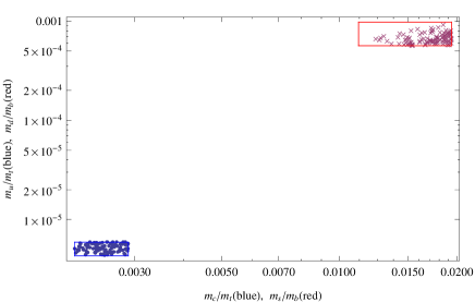
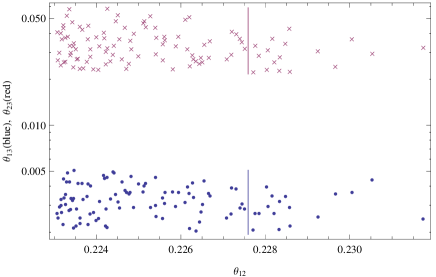
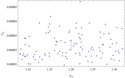
Figure 1: Relations of physical parameters at the GUT scale and they will be allowed by experiments after running to the electroweak scale. The lines denote the allowed region including the threshold corrections $-0.2<{\bar{\eta}}_{b},{\bar{\eta}}_{q}<0.2$ [21]. For $\theta_{12}$ and $\delta_{CP}$, the running effects are small so we take around the best fit values.

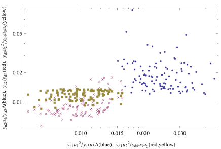
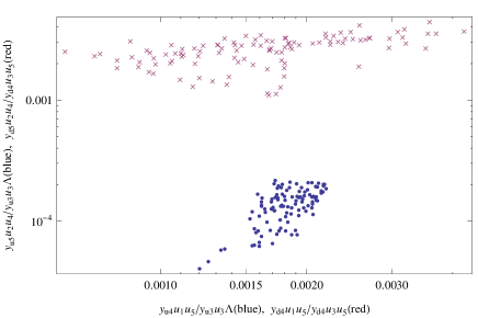
Figure 2: Input values that satisfy the experimentally allowed region indicated by Fig. 1 are displayed. The number of Yukawa couplings is eleven and two parameters are chosen to be common factors to be fixed by the masses of top and bottom. Giving the rest nine parameters with the ratios of the two common factors, we get the physical values. All the Yukawa couplings are considered to be complex and figures show absolute values.

In the figures 1 and 2, we show the random plots. Giving random values for all the Yukawa couplings and VEVs of flavons, we get physical values for masses and mixing by diagonalising mass matrices of up- and down-type quarks. We constrain the results to be consistent with experimental values indicating from Eq. (1). The physical values are actually three up-quark masses, three-down quark masses, three mixing angles, and CP phase. Since the third generation masses can be determined independently, we take mass ratios. For the convenience of numerical calculation, it includes 2$\%$ error for $\theta_{12}$ and 10$\%$ error for $\delta_{\rm CP}$. Expecting higher order corrections, these parameters will have some deviations and the errors will be reasonable. For Jarlskog invariant, we take no constraint and it is calculated by other parameters.

Fig. 2 show the parameter region of all the parameters we use for the mass matrices and all the points satisfy the constraints of Fig. 1. Since the Yukawa couplings are always appeared as the combinations with some flavon VEVs so we take ratios for the parameters with two chosen common factors $y_{u3}u_{3}\Lambda$ for up quarks and $y_{d4}u_{3}u_{5}$ for down quarks. These two parameters can be given by fitting the third generation masses, top and bottom. The left figure indicates NLO corrections which are of order $10^{-2}$ and the right figure is for NNLO corrections which are of order $10^{-3}$. The perturbation for the model seems successful.

6 Summary

We have proposed the first model of quarks in the literature based on the discrete family symmetry $\Delta(6N^{2})$ in which the Cabibbo angle is correctly determined by a residual $Z_{2}\times Z_{2}$ subgroup, and the smaller quark mixing angles may be qualitatively understood from the details of the model. We emphasise that a concrete model is required in order to shed light on the remaining small quark mixing angles $\theta_{23}$ and $\theta_{13}$ which are not fixed by the symmetry alone. In the present model we have performed a full numerical analysis for $N=28$ which shows that all the quark masses and CKM parameters may be accommodated.

Unlike the dihedral groups, $\Delta(6N^{2})$ contains triplet representations and is capable of fixing all the lepton mixing angles using the direct approach. The present model of quarks may therefore be regarded as a first step towards formulating a complete model of quarks and leptons based on $\Delta(6N^{2})$, in which the lepton mixing matrix is fully determined by a Klein subgroup. Taking $N=28$, such a model is capable of predicting $\sin\theta^{\rm MNS}_{13}=0.152$, $\sin\theta^{\rm CKM}_{12}=0.223$ at the leading order. As a general strategy, one can take any value for $\sin\theta^{\rm CKM}_{23}$ without breaking $Z_{2}$ symmetry and the smallest angle $\sin\theta^{\rm CKM}_{13}$ can be derived by NNLO terms which break $Z_{2}$.

References

• [1] J. Beringer et al. (Particle Data Group), Phys. Rev. D 86, 010001 (2012).
• [2] P. F. Harrison, D. H. Perkins and W. G. Scott, Phys. Lett.  B 530, 167 (2002) [arXiv:hep-ph/0202074]; Z. Z. Xing, Phys. Lett. B 533, 85 (2002) [arXiv:hep-ph/0204049]; P. F. Harrison and W. G. Scott, Phys. Lett.  B 535, 163 (2002) [arXiv:hep-ph/0203209]; Phys. Lett.  B 557, 76 (2003) [arXiv:hep-ph/0302025].
• [3] G. Altarelli and F. Feruglio, Rev. Mod. Phys.  82, 2701 (2010) [arXiv:1002.0211 [hep-ph]].
• [4] H. Ishimori, T. Kobayashi, H. Ohki, Y. Shimizu, H. Okada and M. Tanimoto, Prog. Theor. Phys. Suppl.  183, 1 (2010) [arXiv:1003.3552 [hep-th]]; Lect. Notes Phys.  858, 1 (2012); Fortsch. Phys.  61, 441 (2013).
• [5] S. F. King and C. Luhn, Rep. Prog. Phys.  76, 056201 (2013) [arXiv:1301.1340 [hep-ph]].
• [6] S. F. King, A. Merle, S. Morisi, Y. Shimizu and M. Tanimoto, arXiv:1402.4271 [hep-ph].
• [7] C. S. Lam, Phys. Lett. B656, 193 (2007) [arXiv:0708.3665 [hep-ph]]; Phys. Rev. Lett. 101, 121602 (2008) [arXiv:0804.2622 [hep-ph]]; Phys. Rev. D78, 073015 (2008) [arXiv:0809.1185 [hep-ph]]; W. Grimus, L. Lavoura and P. O. Ludl, J. Phys. G36, 115007 (2009) [arXiv:0906.2689 [hep-ph]].
• [8] DAYA-BAY Collaboration, Phys. Rev. Lett. 108, 171803 (2012) [arXiv:1203.1669 [hep-ex]]; Chin. Phys. C 37, 011001 (2013) [arXiv:1210.6327 [hep-ex]]; DOUBLE-CHOOZ Collaboration, Phys. Rev. Lett. 108, 131801 (2012) [arXiv:1112.6353 [hep-ex]]; RENO Collaboration, Phys. Rev. Lett. 108, 191802 (2012) [arXiv:1204.0626 [hep-ex]].
• [9] T2K Collaboration, Phys. Rev. Lett. 107, 041801 (2011) [arXiv:1106.2822 [hep-ex]]; MINOS Collaboration, Phys. Rev. Lett. 107, 181802 (2011) [arXiv:1108.0015 [hep-ex]].
• [10] S. F. King, T. Neder and A. J. Stuart, Phys. Lett. B 726 (2013) 312 [arXiv:1305.3200 [hep-ph]].
• [11] C. S. Lam, Phys. Lett. B 656 (2007) 193 [arXiv:0708.3665 [hep-ph]].
• [12] A. Blum, C. Hagedorn and M. Lindner, Phys. Rev. D 77 (2008) 076004 [arXiv:0709.3450 [hep-ph]].
• [13] J. E. Kim and M. -S. Seo, JHEP 1102 (2011) 097 [arXiv:1005.4684 [hep-ph]].
• [14] A. Blum and C. Hagedorn, Nucl. Phys. B 821 (2009) 327 [arXiv:0902.4885 [hep-ph]].
• [15] A. Blum, C. Hagedorn and A. Hohenegger, JHEP 0803 (2008) 070 [arXiv:0710.5061 [hep-ph]].
• [16] C. Hagedorn and D. Meloni, Nucl. Phys. B 862 (2012) 691 [arXiv:1204.0715 [hep-ph]].
• [17] M. Holthausen and K. S. Lim, Phys. Rev. D 88 (2013) 033018 [arXiv:1306.4356 [hep-ph]].
• [18] T. Araki, H. Ishida, H. Ishimori, T. Kobayashi and A. Ogasahara, Phys. Rev. D 88 (2013) 096002 [arXiv:1309.4217 [hep-ph]].
• [19] S. F. King, JHEP 1401 (2014) 119 [arXiv:1311.3295 [hep-ph]].
• [20] J. A. Escobar and C. Luhn, J. Math. Phys.  50 (2009) 013524 [arXiv:0809.0639 [hep-th]].
• [21] S. Antusch and V. Maurer, JHEP 1311 (2013) 115 [arXiv:1306.6879 [hep-ph]].