An importance sampling approach for copula models in insurance

Abstract

An importance sampling approach for sampling copula models is introduced. We propose two algorithms that improve Monte Carlo estimators when the functional of interest depends mainly on the behaviour of the underlying random vector when at least one of the components is large. Such problems often arise from dependence models in finance and insurance. The importance sampling framework we propose is general and can be easily implemented for all classes of copula models from which sampling is feasible. We show how the proposal distribution of the two algorithms can be optimized to reduce the sampling error. In a case study inspired by a typical multivariate insurance application, we obtain variance reduction factors between 10 and 30 in comparison to standard Monte Carlo estimators.
Key words: Copula, Dependence models, Importance sampling, Insurance, Risk measure, Tail event

1 Introduction

Many insurance applications, see our motivation Section 2, lead to the problem of calculating a functional of the form $\mathbb{E}[\Psi_{0}(\mathbf{X})]$, where $\mathbf{X}=(X_{1},\dots,X_{d}):\Omega\rightarrow\mathbb{R}^{d}$ is a random vector on a probability space $(\Omega,\mathcal{F},\mathbb{P})$ and $\Psi_{0}:\mathbb{R}^{d}\rightarrow\mathbb{R}$ is a measurable function. If the components of $\mathbf{X}$ cannot be assumed to be independent, it is popular to model the distribution of $\mathbf{X}$ with a copula, such that

$$\mathbb{P}\left[X_{1}\leq x_{1},\dots,X_{d}\leq x_{d}\vphantom{x_{1,}}\right]=C\left(\vphantom{1_{1_{1}}}F_{X_{1}}(x_{1}),\dots,F_{X_{d}}(x_{d})\right),\qquad\mathbf{x}\in\mathbb{R}^{d},$$

where $F_{X_{j}}(x)=\mathbb{P}[X_{j}\leq x]$, $j=1,\dots,d$, are the marginal cumulative distribution functions (cdf) and $C:[0,1]^{d}\rightarrow[0,1]$ is a copula. A copula allows one to separate the dependence structure from the marginal distributions, which is useful for constructing multivariate stochastic models. We assume the reader to have a basic knowledge on copulas and refer to McNeil et al., (2005) or Nelsen, (2006) for introductions.

The usual approach to estimate $\mathbb{E}[\Psi_{0}(\mathbf{X})]$ is by Monte Carlo simulation. In actuarial practice, very often a set of outcomes of $\mathbf{X}$ with a low probability makes a large contribution to $\mathbb{E}[\Psi_{0}(\mathbf{X})]$. In this case, importance sampling can increase the number of samples lying in this set. Through a weighting approach, an unbiased estimator with a reduced variance can be obtained.

Importance sampling for copulas has been investigated by Glasserman and Li, (2005) and Huang et al., (2010) for the Gauss copula only and Bee, (2011) for absolutely continuous copulas. These papers are inspired by copula models in financial applications and assume the copula to be either Gaussian or having a known density. Copulas used in insurance however often deviate from these assumptions.

The main contribution of this paper is the study of importance sampling techniques that do not rely on a specific copula structure. We consider the case where the functional $\Psi_{0}$ of interest depends mainly on the behaviour of the random vector $\mathbf{X}$ when at least one of the components is large. Such problems often arise from dependence models in the realm of finance and insurance, where distorted expectations of heavy tailed distributions are involved. We propose a new importance sampling framework for this setup which can be implemented for all classes of copula models from which sampling is feasible.

This paper is organized as follows. After motivating our work in Section 2, we introduce the importance sampling approach in Section 3. Section 4 presents a rejection sampling algorithm while Section 5 presents a direct sampling algorithm. For each of them, we expose the sampling of the proposal distribution, the calculation of the importance sampling weights and we discuss the optimal choice of the proposal distribution. Section 6 discusses the efficiency of our algorithms in rare event settings. A case study is given in Section 7 and Section 8 concludes.

2 Motivation

In a copula model, we may write

$$\mathbb{E}[\Psi_{0}(\mathbf{X})]=\mathbb{E}[\Psi(\mathbf{U})]$$

where $\mathbf{U}=(U_{1},\dots,U_{d}):\Omega\rightarrow\mathbb{R}^{d}$ is a random vector with distribution function $C$, $\Psi:[0,1]^{d}\rightarrow\mathbb{R}$ is defined as

$$\Psi(u_{1},\dots,u_{d})=\Psi_{0}\left(F_{X_{1}}^{-1}(u_{1}),\dots,F_{X_{d}}^{-1}(u_{d})\right),$$

and $F_{X_{j}}^{-1}(p)=\inf\{x\in\mathbb{R}:F_{X_{j}}(x)\geq p\}$, for $j=1,\dots,d$.

If $C$ and the margins $F_{X_{j}}$ are known, we can use Monte Carlo simulation to estimate $\mathbb{E}[\Psi(\mathbf{U})]$. For a random sample $\{\mathbf{U}_{i}:i=1,\dots,n\}$ of $\mathbf{U}$, the Monte Carlo estimator of $\mathbb{E}[\Psi(\mathbf{U})]$ is given by

$$\mu_{n} =\frac{1}{n}\sum_{i=1}^{n}\Psi(\mathbf{U}_{i}).$$ (2.1)

In this paper, we consider the case where $\Psi$ is large only when at least one of its arguments is close to $1$, or equivalently, if at least one of the components of $\mathbf{X}$ is large. This assumption is inspired by several applications in insurance, as the following examples illustrate:

• The fair premium of a stop loss cover with deductible $T$ is $\mathbb{E}\left[\max\left\{\sum_{j=1}^{d}X_{j}-T,0\right\}\right]$. The corresponding functional is $\Psi(\mathbf{u})=\max\left\{\sum_{j=1}^{d}F_{X_{j}}^{-1}(u_{j})-T,0\right\}$; see the left hand side of Figure 1 for a contour plot of $\Psi$ for two Pareto margins.

  

  

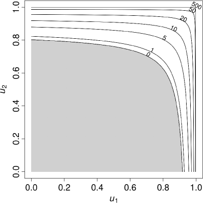
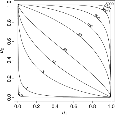
  Figure 1: Left: Contour lines for the excess function $\Psi(u_{1},u_{2})=\max\{F_{X_{1}}^{-1}(u_{1})+F_{X_{2}}^{-1}(u_{2})-10,0\}$, where the margins are Pareto distributed with $F_{X_{1}}(x)=1-(1+x/4)^{-2}$ and $F_{X_{2}}(x)=1-(1+x/8)^{-2}$. The grey area indicates where $\Psi$ is zero. Right: Contour lines for the product function $\Psi(u_{1},u_{2})=F_{X_{1}}^{-1}(u_{1})F_{X_{2}}^{-1}(u_{2})$, where $X_{1}\sim\operatorname{LN}(2,1)$ and $X_{2}\sim\operatorname{LN}(1,1.5)$.

• Risk measures for an aggregate $S=\sum_{j=1}^{d}X_{j}$, such as Value-at-Risk, $\operatorname{VaR}_{\alpha}(S)$, or Expected Shortfall, $\operatorname{ES}_{\alpha}(S)$, $\alpha\in(0,1)$, cannot in general be written as an expectation of type $\mathbb{E}[\Psi_{0}(\mathbf{X})]$. However, they are functionals of the aggregate distribution function $F_{S}(x)=\mathbb{P}[S\leq x]=\mathbb{E}[\Psi^{(x)}(\mathbf{U})]$, where $\Psi^{(x)}$ $(x\in\mathbb{R})$ is the indicator function

  $$\Psi^{(x)}(\mathbf{u})=\mathbf{1}\left\{F_{X_{1}}^{-1}(u_{1})+\dots+F_{X_{d}}^{-1}(u_{d})\leq x\right\}.$$

  We can therefore write

  $$\operatorname{VaR}_{\alpha}(S)=\inf\left\{x\in\mathbb{R}:\mathbb{E}[\Psi^{(x)}(\mathbf{U})]\geq\alpha\right\},\qquad\operatorname{ES}_{\alpha}(S)=\frac{1}{1-\alpha}\int_{\alpha}^{1}\operatorname{VaR}_{u}(S)\mathrm{d}u,$$

  which depend only on those $x$ for which $\mathbb{E}[\Psi^{(x)}(\mathbf{U})]\geq\alpha$ holds. This is determined by the tail behaviour of $S$, which is strongly influenced by the properties of the copula $C$ when at least one component is close to $1$. Note that capital allocation methods such as the Euler principle for Expected Shortfall behave similarly, see Tasche, (2008) and McNeil et al., (2005), page 260.

• Computing the covariance (or correlation) of two positive heavy-tailed random variables $X_{1}$ and $X_{2}$ requires the calculation of $\mathbb{E}[X_{1}X_{2}]$. The implied functional is $\Psi(u_{1},u_{2})=F_{X_{1}}^{-1}(u_{1})F_{X_{2}}^{-1}(u_{2})$. A contour plot of $\Psi$ for log-normal (LN) margins is shown in the right hand side of Figure 1. In contrast to the preceding examples, this $\Psi$ does not only depend on the tail behaviour of $(X_{1},X_{2})$. However, $\mathbb{E}[\Psi(\mathbf{U})]$ depends mainly on the copula behaviour when at least one argument is close to 1, as $\Psi$ becomes large in this case.

Note that in this framework we follow the convention of (McNeil et al.,, 2005, Remark 2.1) that $\mathbf{X}$ refers to a loss and $-\mathbf{X}$ to a profit, which is more common in an actuarial context. One could have equally well worked with the P&L random variable $-\mathbf{X}$ by changing the area of interest to where components of $\mathbf{X}$ are small.

3 Importance sampling

The idea behind importance sampling is to sample from a proposal distribution $F_{\mathbf{V}}$ different from the target distribution $C.$ The proposal distribution concentrates more samples in the region driving large contributions to $\mathbb{E}[\Psi(\mathbf{U})]$. With a suitable weighting approach, one obtains an unbiased estimator with lower variance.

Suppose the function $\Psi$ under consideration is in the class illustrated above: $\Psi$ is large if at least one of its arguments is close to $1$. In this case, a drawback of the estimator $\mu_{n}$ in (2.1) is that, typically, for many of the samples $\mathbf{U}_{i}$, none of the components is close to $1$. Therefore, most samples lie in a region of low interest. The estimation error of $\mu_{n}$ can thus be large, even if $n$ is large.

Let $\mathbf{V}=(V_{1},\dots,V_{d}):\Omega\rightarrow[0,1]^{d}$ denote a random vector with distribution function $F_{\mathbf{V}}$. We can rewrite the integral $\mathbb{E}[\Psi(\mathbf{U})]$ as

$$\mathbb{E}[\Psi(\mathbf{U})]=\int_{[0,1]^{d}}\Psi(\mathbf{u})\mathrm{d}C(\mathbf{u})=\int_{[0,1]^{d}}\Psi(\mathbf{u})\frac{\mathrm{d}C(\mathbf{u})}{\mathrm{d}F_{\mathbf{V}}(\mathbf{u})}\mathrm{d}F_{\mathbf{V}}(\mathbf{u})=\mathbb{E}\left[\Psi(\mathbf{V})\frac{\mathrm{d}C(\mathbf{V})}{\mathrm{d}F_{\mathbf{V}}(\mathbf{V})}\right],$$ (3.1)

where $\mathrm{d}C/\mathrm{d}F_{\mathbf{V}}$ denotes the Radon–Nikodym derivative of $C$ with respect to $F_{\mathbf{V}}$. The Radon–Nikodym derivative exists if and only if the copula $C$ is absolutely continuous with respect to $F_{\mathbf{V}}$. We will provide more details on this issue later in this section. If $C$ and $F_{\mathbf{V}}$ are absolutely continuous with densities $c$ and $f_{\mathbf{V}}$ with respect to the Lebesgue measure, the Radon–Nikodym derivative $\mathrm{d}C/\mathrm{d}F_{\mathbf{V}}$ is simply the ratio of the densities $c/f_{\mathbf{V}}$.

For an i.i.d. sample $\{\mathbf{V}_{i}:i=1,\dots,n\}$ of $\mathbf{V}$, we can define the importance sampling estimator

$$\widehat{\mu}_{n}=\frac{1}{n}\sum_{i=1}^{n}\Psi(\mathbf{V}_{i})w(\mathbf{V}_{i}),$$ (3.2)

where $w(\mathbf{V}_{i})=\mathrm{d}C(\mathbf{V}_{i})/\mathrm{d}F_{\mathbf{V}}(\mathbf{V}_{i})$ are the sample weights. The goal is then to find $F_{\mathbf{V}}$ such that the variance of $\widehat{\mu}_{n}$ is smaller than the variance of $\mu_{n}$.

In order to define the proposal distribution $F_{\mathbf{V}},$ we suggest a mixing approach by taking a weighted average of a multivariate cdf $C^{[\lambda]}:[0,1]^{d}\rightarrow[0,1]$ over different values of $\lambda$. Let $F_{\Lambda}$ denote the distribution function of a random variable $\Lambda:\Omega\mapsto[0,1)$. We then define the distribution $F_{\mathbf{V}}$ of $\mathbf{V}$ as a mixture of $C^{[\lambda]}$ over the distribution $F_{\Lambda}$:

$$F_{\mathbf{V}}(\mathbf{u})=\int_{0}^{1}C^{[\lambda]}(\mathbf{u})\,\mathrm{d}F_{\Lambda}(\lambda),\quad\mathbf{u}\in[0,1]^{d}.$$

The distribution $C^{[\lambda]}$ shall be understood as a distorted version of the copula $C$ that will concentrate samples in specific regions of the sampling space. These regions will then be parametrized by the value of $\lambda$. More precisely, we will construct $C^{[\lambda]}$ so that it puts mass only in the region $[0,1]^{d}\setminus[0,\lambda]^{d}$. In the sequel, we will propose two possible definitions of $C^{[\lambda]}$ that will define two importance sampling algorithms, namely a rejection sampling algorithm in Section 4 and a direct sampling algorithm in Section 5.

We will see that this mixture approach is natural in order to allow $C$ to be absolutely continuous with respect to $F_{\mathbf{V}}$. In particular, the absolute continuity is guaranteed for any copula $C$ if the following condition is satisfied.

Condition A.

The random variable $\Lambda$ satisfies $\mathbb{P}[\Lambda=0]>0$.

In order to obtain a well defined weight function $w(\mathbf{V})$ and an unbiased estimator $\widehat{\mu}_{n}$, Condition A must be fulfilled. This condition does not require particular assumptions on $C$. Although it seems restrictive, we will see that it is also needed to have a consistent estimator $\widehat{\mu}_{n}$. To that end, we assume Condition A to be satisfied in what follows.

The construction of the proposal distribution $F_{\mathbf{V}}$ as a $C^{[\lambda]}$-mixture directly yields a sampling method, as one can draw a realization of $F_{\mathbf{V}}$ by first drawing $\Lambda\sim F_{\Lambda}$ and then $\mathbf{V}\sim C^{[\Lambda]}$. Therefore, the following algorithm can be used to calculate $\widehat{\mu}_{n}$:

Algorithm 3.1.

Fix $n\in\mathbb{N}$. For $i=1,\dots,n$, do:

1. draw $\Lambda_{i}\sim F_{\Lambda}$;

2. draw $\mathbf{V}_{i}\sim C^{[\Lambda_{i}]}$;

3. calculate $w(\mathbf{V}_{i})$;

Return $\widehat{\mu}_{n}=n^{-1}\sum_{i=1}^{n}\Psi(\mathbf{V}_{i})w(\mathbf{V}_{i})$.

The following lemma establishes consistency and asymptotic normality of the estimator $\widehat{\mu}_{n}$.

Lemma 3.2.

Suppose that $\operatorname{var}[\Psi(\mathbf{U})]<\infty$ and that $w(\,\cdot\,)\leq B$ for some constant $B<\infty$. Then

1. $\widehat{\mu}_{n}$ converges $\mathbb{P}$-almost surely to $\mu$;

2. $\sigma^{2}=\operatorname{var}[\Psi(\mathbf{V})w(\mathbf{V})]<\infty$ and $n^{1/2}(\widehat{\mu}_{n}-\mu)$ converges to $\mathcal{N}(0,\sigma^{2})$ in distribution.

Proof.

1. Since $\mathbb{E}[\Psi(\mathbf{V})w(\mathbf{V})]=\mathbb{E}[\Psi(\mathbf{U})]$, consistency follows directly from the Strong Law of Large Numbers.

2. Note that

   $$\mathbb{E}\left[\Psi(\mathbf{V})^{2}w(\mathbf{V})^{2}\right]=\mathbb{E}\left[\Psi(\mathbf{U})^{2}w(\mathbf{U})\right]\leq\mathbb{E}\left[\Psi(\mathbf{U})^{2}\right]B<\infty,$$

   where the first equality is justified by a change of measure, see (3.1). We can immediately deduce asymptotic normality of $\widehat{\mu}_{n}$ by the Central Limit Theorem, see, for example, Section 2.4 in Durrett, (2010), page 110. $\hfill\Box$

We will later show that under some mild assumptions on $F_{\Lambda}$, the weight function will indeed be bounded on $[0,1]$.

4 A rejection sampling algorithm

For this algorithm, we propose $C^{[\lambda]}$ to denote the distribution of $\mathbf{U}$ conditioned on the event that at least one of its components exceeds $\lambda$:

$$C^{[\lambda]}(\mathbf{u}) =\mathbb{P}\left[U_{1}\leq u_{1},\dots,U_{d}\leq u_{d}\,\left|\,\max\{U_{1},\dots,U_{d}\}>\lambda\right.\right]=\mathbb{P}[U_{1}\leq u_{1},\dots,U_{d}\leq u_{d}\,|\,\mathbf{U}\notin[0,\lambda]^{d}]$$

$$=\frac{C(\mathbf{u})-C\left(\min\{u_{1},\lambda\},\dots,\min\{u_{d},\lambda\}\right)}{1-C(\lambda\mathbf{1})},$$

where $\lambda\mathbf{1}=\lambda(1,\dots,1)=(\lambda,\dots,\lambda)\in[0,1)^{d}$. Note that $C^{[\lambda]}$ is a copula only if $C(\lambda\mathbf{1})=0$, but $C^{[\lambda]}$ does not need to be copula for our algorithm to work. By putting mass of $\Lambda$ on $(0,1)$, we can put more weight on the region of the copula where at least one component is large. For instance, if $F_{\Lambda}$ is discrete and $\mathbb{P}[\Lambda=0]=\mathbb{P}[\Lambda=0.9]=0.5$, then 50% of the samples of $\mathbf{V}$ are constrained to lie only in $[0,1]^{d}\setminus[0,0.9]^{d}$ while the other 50% of the samples will lie on $[0,1]^{d}$. Note that the mass on $[0,1]^{d}\setminus[0,0.9]^{d}$ would then be higher than 50%. On the other hand, the case $\mathbb{P}[\Lambda=0]=1$ yields $F_{\mathbf{V}}=C$.

4.1 Sampling the proposal distribution

We shall now describe how samples from $F_{\mathbf{V}}$ can be drawn. As $F_{\mathbf{V}}$ is defined through a mixing distribution, drawing a realization from $F_{\mathbf{V}}$ is done by drawing first $\Lambda\sim F_{\Lambda}$ and then $\mathbf{V}\sim C^{[\Lambda]}$, see Algorithm 3.1. Unfortunately, for well-known copula classes, the conditional distribution $C^{[\lambda]}$ is not analytically tractable. We are aware of only one class of shock copulas, namely Marshall–Olkin copulas, for which it is possible to sample directly from the conditional distribution $C^{[\lambda]}$. Details and the corresponding algorithm are provided in Appendix A.

However, sampling from $C^{[\lambda]}$ for an arbitrary copula $C$ is always possible through a rejection algorithm, which is simple to implement but may be time consuming due to the rejection step. With the following rejection algorithm, it is thus possible to draw a sample from $F_{\mathbf{V}}$ for any copula $C$. The only condition is that it is feasible to draw realizations from both $F_{\Lambda}$ and $C$. It is not necessary to know further properties of $C$, such as its density. The basic idea is to first draw a realization $\Lambda$ from $F_{\Lambda}$ and then iteratively draw realizations from $C$ until one obtains a maximum component larger than $\Lambda$.

Algorithm 4.1.

To draw one realization of $F_{\mathbf{V}}$:

1. draw $\Lambda\sim F_{\Lambda}$;

2. repeatedly draw $\mathbf{V}\sim C$ until $\max\{V_{1},\dots,V_{d}\}>\Lambda$;

3. return $\mathbf{V}$.

A disadvantage of Algorithm 4.1 is that typically many samples of $C$ are discarded, because of the acceptance condition in Step 2. In practice, there are two important reasons why this approach can be justified over standard Monte-Carlo. First, the evaluation of $\Psi$ can be numerically more expensive than sampling from the copula, if, for instance, marginal quantile functions are demanding to compute or if $\Psi_{0}$ has no closed form. Second, storing a large sample of $\mathbf{U}$ in computer memory can be numerically more expensive than generating it. This case may appear for example in estimating allocated capital, which requires storing the whole multivariate sample. In particular in high dimensional problems, memory constraints can be quite prohibitive. For illustration, consider the following example: for the calculation of risk capital and risk contributions in a setting with heavy tailed marginals, a sample of size 10’000’000 is often not large enough to yield sufficiently small estimation errors. However, in a 1’000-dimensional setting with double-precision floating point numbers, this sample would require about 80 gigabytes of memory, which is more than an average computer currently possesses in terms of RAM.

Algorithm 4.1 may require several realizations from $\mathbf{U}$ in order to generate one realization of $\mathbf{V}$. The following lemma gives an expression for the expected number of $\mathbf{U}$’s for obtaining a realization of $\mathbf{V}$.

Lemma 4.2.

Let $N_{\mathbf{V}}$ denote the number of draws from $C$ necessary to simulate one realization from $F_{\mathbf{V}}$. The expected number of draws is

$$\mathbb{E}[N_{\mathbf{V}}]=\int_{0}^{1}\frac{1}{1-C(\lambda\mathbf{1})}\mathrm{d}F_{\Lambda}(\lambda).$$

Proof. The probability that one draw from $\mathbf{U}\sim C$ satisfies $\max\{U_{1},\dots,U_{d}\}>\lambda$ is $\mathbb{P}[\max\{U_{1},\dots,U_{d}\}>\lambda]=1-C(\lambda\mathbf{1})$. Therefore, the number of draws necessary to simulate from $C^{[\lambda]}$ for a fixed $\lambda$ is geometrically distributed with parameter $1-C(\lambda\mathbf{1})$ and has expectation $1/[1-C(\lambda\mathbf{1})]$. In order to simulate from $\mathbf{V}$, $\Lambda$ is drawn from $F_{\Lambda}$. Therefore, $\mathbb{E}[N_{\mathbf{V}}]$ is given by averaging $1/[1-C(\lambda\mathbf{1})]$ over $F_{\Lambda}$. $\hfill\Box$

Using the Fréchet–Höffding bounds (see Theorem 5.7 in McNeil et al., (2005)), we can give the following bounds for $\mathbb{E}[N_{\mathbf{V}}]$, which depend only on $F_{\Lambda}$ and the dimension $d$, independent of the copula $C$.

Theorem 4.3.

We have

$$\frac{1}{d}\mathbb{E}\left[\frac{1}{1-\Lambda}\right]\leq\mathbb{E}[N_{\mathbf{V}}]\leq\mathbb{E}\left[\frac{1}{1-\Lambda}\right].$$

Proof. Due to the upper Fréchet–Höffding bound, we have $C(\lambda\mathbf{1})\leq\min\{\lambda,\dots,\lambda\}=\lambda$. Hence,

$$\mathbb{E}[N_{\mathbf{V}}] =\int_{0}^{1}\frac{1}{1-C(\lambda\mathbf{1})}\mathrm{d}F_{\Lambda}(\lambda)\leq\int_{0}^{1}\frac{1}{1-\lambda}\mathrm{d}F_{\Lambda}(\lambda)=\mathbb{E}\left[\frac{1}{1-\Lambda}\right].$$

Analogously, due to the lower Fréchet–Höffding bound:

$$\mathbb{E}[N_{\mathbf{V}}]\geq\int_{0}^{1}\frac{1}{1-\max\{0,d\lambda-d+1\}}\mathrm{d}F_{\Lambda}(\lambda)=\int_{0}^{1}\max\left\{1,\frac{1}{d(1-\lambda)}\right\}\mathrm{d}F_{\Lambda}(\lambda)\geq\frac{1}{d}\mathbb{E}\left[\frac{1}{1-\Lambda}\right].\qquad\hfill\Box$$

Due to Theorem 4.3, the number of draws from $C$ necessary to draw one realization from $\mathbf{V}$ has a finite expectation if and only if $\mathbb{E}[(1-\Lambda)^{-1}]<\infty$. Intuitively, this implies that $\Lambda$ should not have mass concentrated near 1 in order to be able to use Algorithm 4.1.

We shall see in the next section that specific choices for the copula $C$ and for $F_{\Lambda}$ will allow us to find analytical expressions for $\mathbb{E}[N_{\mathbf{V}}]$.

4.2 Calculation of sample weights

This section outlines how the weights $w(\mathbf{V}_{i})$ used in Algorithm 3.1 can be calculated. We first deduce a useful representation.

Theorem 4.4.

The Radon–Nikodym derivative $w(\mathbf{u})=\mathrm{d}C(\mathbf{u})/\mathrm{d}F_{\mathbf{V}}(\mathbf{u})$ can be written as

$$w(\mathbf{u})=\left(\int_{0}^{\max\{u_{1},\dots,u_{d}\}}\frac{1}{1-C(\lambda\mathbf{1})}\mathrm{d}F_{\Lambda}(\lambda)\right)^{-1}.$$

Proof. Due to the Leibnitz integral rule, we have $\mathrm{d}F_{\mathbf{V}}(\mathbf{u})=\int_{0}^{1}\mathrm{d}C^{[\lambda]}(\mathbf{u})\mathrm{d}F_{\Lambda}(\lambda)$. From the definition of $C^{[\lambda]}$, we can deduce the differential

$$\mathrm{d}C^{[\lambda]}(\mathbf{u})=\begin{cases}0,&\mathbf{u}\in[0,\lambda]^{d},\\ \frac{\mathrm{d}C(\mathbf{u})}{1-C(\lambda\mathbf{1})},&\text{ otherwise. }\end{cases}$$

Using both identities, we obtain

$$\mathrm{d}F_{\mathbf{V}}(\mathbf{u})=\mathrm{d}C(\mathbf{u})\int_{0}^{1}\frac{\mathbf{1}\left\{\lambda\leq\max\{u_{1},\dots,u_{d}\}\right\}}{1-C(\lambda\mathbf{1})}\mathrm{d}F_{\Lambda}(\lambda),$$

leading to the desired result. $\hfill\Box$

The efficiency of our approach comes from the fact that the term $\mathrm{d}C(\mathbf{u})$ does not appear in $w(\mathbf{u})$. For instance, if $C$ is absolutely continuous with respect to the Lebesgue measure, the density of $C$ does not have to be evaluated to calculate $w(\mathbf{u})$. This is in an advantage in comparison to most other importance sampling algorithms, for which the existence of the density of $C$ is required.

In order to simplify the notation, let $\widetilde{w}(t):[0,1]\rightarrow[0,\infty)$ be defined as

$$\widetilde{w}(t)=\left(\int_{0}^{t}\frac{1}{1-C(\lambda\mathbf{1})}\mathrm{d}F_{\Lambda}(\lambda)\right)^{-1},$$

such that $w(\mathbf{u})=\widetilde{w}(\max\{u_{1},\dots,u_{d}\})$.

Lemma 4.5.

Under Condition A, $\widetilde{w}$ is bounded from above by $\mathbb{P}[\Lambda=0]^{-1}$ on $[0,1].$

Proof. Since $C(\lambda\mathbf{1}),\lambda\in[0,1]$, the diagonal section of the copula $C$ and the distribution function $F_{\Lambda}$ are both increasing functions, the weight function $\widetilde{w}(t)$ is decreasing on $[0,1]$, it is therefore bounded above by $\widetilde{w}(0)=\mathbb{P}[\Lambda=0]^{-1}<\infty.$ $\hfill\Box$

As a consequence, Condition A is not only sufficient to obtain existence of the weights, but it also guarantees that they are bounded. In virtue of Lemma 3.2, this is needed for consistency and asymptotic normality of the importance sampling estimator.

For general $C$ and $F_{\Lambda}$, the evaluation of the weight function $\widetilde{w}$ can be demanding. In general, numerical integration schemes could be used. To circumvent these problems, we present two cases in which the evaluation of $\widetilde{w}$ is straightforward. Section 4.2.1 illustrates the case in which $F_{\Lambda}$ is discrete. In Section 4.2.2, we assume that the copula $C$ lies in a large class of copulas satisfying a polynomial condition on the diagonal. For this class, there is a specific choice of $F_{\Lambda}$ which leads to an analytical expression for $\widetilde{w}$.

4.2.1 Discrete $F_{\Lambda}$

This section shows that in the case of a discrete $F_{\Lambda}$, calculating $\widetilde{w}(t)$ is fast and can easily be implemented. To this end, suppose $F_{\Lambda}$ is discrete with a finite number $n_{\Lambda}$ of atoms:

$$\mathbb{P}[\Lambda=x_{k}]=p_{k},k=1,\dots,n_{\Lambda},\sum_{k=1}^{n_{\Lambda}}p_{k}=1,p_{1}>0,\text{ and }0=x_{1}<\dots<x_{n_{\Lambda}}<1.$$

Note that Condition A is satisfied. In this case, $\widetilde{w}$ can be written as a step function

$$\widetilde{w}(t)=\left(\sum_{k=1}^{n_{\Lambda}}\frac{\mathbf{1}\{x_{k}\leq t\}}{1-C(x_{k}\mathbf{1})}p_{k}\right)^{-1}.$$ (4.1)

In order to evaluate $\widetilde{w}(t)$, it is sufficient to calculate (or approximate) $C(x_{k}\mathbf{1})$ for $k=1,\dots,n_{\Lambda}$. These values must be calculated only once for the whole sample. This approach with a discrete $F_{\Lambda}$ can be used for any copula $C$. For $\mathbb{E}[N_{\mathbf{V}}]$, we obtain the explicit expression

$$\mathbb{E}[N_{\mathbf{V}}]=\sum_{k=1}^{n_{\Lambda}}\frac{p_{k}}{[1-C(x_{k}\mathbf{1})]}.$$

4.2.2 Continuous $F_{\Lambda}$

For continuous $F_{\Lambda}$, the weight function $\widetilde{w}$ can in general only be calculated numerically. In the following, we assume that both $C$ and $F_{\Lambda}$ are of a special polynomial form, which leads to an explicit $\widetilde{w}$. Suppose that $C$ behaves as a monomial on its diagonal:

$$C(u\mathbf{1})=u^{\alpha},\quad 0\leq u\leq 1.$$

Due to the Fréchet–Höffding bounds, $\alpha$ must satisfy $1\leq\alpha\leq d$. This class of copulas is quite large. The following list shows some popular copula families satisfying this condition.

• Marshall–Olkin copulas as proposed in Example A.2 of Appendix A. The corresponding exponent is $\alpha=\sum_{j=1}^{m}\min_{i:j\in I_{i}}(s_{j}/\widetilde{s}_{i})$.

• Sibuya copulas, as defined in Hofert and Vrins, (2013), for which the default rate process is a homogeneous Poisson process.

• Extreme value copulas with a Pickands dependence function $A$. The corresponding exponent is $\alpha=dA(1/d,\dots,1/d)$; see Section 7 in McNeil et al., (2005) for a definition of extreme value copulas. Note that this class contains the well-known Gumbel copula, for example.

Apart from the copula $C$, we also make some specific assumptions about $F_{\Lambda}:[0,1]\rightarrow[0,1]$. Suppose that

$$F_{\Lambda}(\lambda)=(1-\gamma)+\gamma\left(1-(1-\lambda^{\alpha})^{\beta}\right),\quad\beta>1,\,0\leq\gamma\leq 1.$$

The parameter $\alpha$ is given by the exponent of the copula diagonal, so cannot be chosen freely. Furthermore, $F_{\Lambda}$ has an atom of weight $1-\gamma$ at zero. This distribution is similar to the distribution of Kumaraswamy, (1980). In this case, the weight function can easily be calculated as

$$\widetilde{w}(t)=\left(1-\gamma+\gamma\beta\int_{0}^{t}\alpha\lambda^{\alpha-1}(1-\lambda^{\alpha})^{\beta-2}\mathrm{d}\lambda\right)^{-1}=\frac{\beta-1}{\beta-1+\gamma\left(1-\beta(1-t^{\alpha})^{\beta-1}\right)}.$$ (4.2)

As $\mathbb{E}[N_{\mathbf{V}}]=1/\widetilde{w}(1)$ (c.f. Lemma 4.2), we obtain an explicit expression for $\mathbb{E}[N_{\mathbf{V}}]$:

$$\mathbb{E}[N_{\mathbf{V}}]=1+\frac{\gamma}{\beta-1}.$$ (4.3)

In order for Condition A to be satisfied, we assume $\gamma<1$. In fact, using properties of the hypergeometric function, it is possible to show that for $\gamma=1$, the weight function is unbounded and the variance of the weights $\operatorname{var}[w(\mathbf{V})]$ is always infinite.

There are many copula classes which have an explicit diagonal. For instance, the Clayton family has a diagonal $C(t\mathbf{1})=(dt^{-\theta}-d+1)^{-1/\theta}$ for some $0<\theta<\infty$. For future research, we may point out that it would be interesting to find “conjugate” $F_{\Lambda}$ for copulas that also allow for an explicit form of $\widetilde{w}(\cdot)$.

4.3 Optimal proposal distribution

This section gives an approach to calibrate the distribution $F_{\Lambda}$ to the problem at hand. The basic idea is to choose the proposal distribution $F_{\mathbf{V}}$ in such a way that $\widehat{\mu}_{n}$ has a smaller variance than $\mu_{n}$. In our case, this reduces to optimally choosing the distribution $F_{\Lambda}$. In general, $F_{\Lambda}$ must have an atom at $0$ in order to satisfy Condition A. If Algorithm 4.1 is used for sampling, we also need to fulfill the constraint that $\mathbb{E}[1/(1-\Lambda)]$ is not too large, and, in particular, finite.

Zero variance (i.e., no estimation error) would be obtained for $\widehat{\mu}_{n}$ if

$$\Psi(\mathbf{u})w(\mathbf{u})=\mathbb{E}[\Psi(\mathbf{U})],\quad\mathbf{u}\in[0,1)^{d},$$ (4.4)

see Section 4.1 in Asmussen and Glynn, (2007), page 128. This choice is obviously not possible as $\mathbb{E}[\Psi(\mathbf{U})]$ is unknown. To obtain a small variance, we should choose $\Lambda$ such that $w(\mathbf{u})^{-1}$ is approximately proportional to $\Psi(\mathbf{u})$. Due to Theorem 4.4, we may write this relation as

$$K\int_{0}^{\max\{u_{1},\dots,u_{d}\}}\frac{1}{1-C(\lambda\mathbf{1})}\mathrm{d}F_{\Lambda}(\lambda)\approx\Psi(\mathbf{u}),$$ (4.5)

for some unknown constant $K\in\mathbb{R}_{+}$. In order to obtain a tractable optimization scheme, we use our assumption that $\Psi(\mathbf{u})$ is large if at least one of its components is large, namely

$$\Psi(\mathbf{u})\approx\Psi\bigl{(}\max\{u_{1},\dots,u_{d}\}\mathbf{1}\bigr{)}.$$ (4.6)

Plugging (4.6) into (4.5), we obtain

$$K\int_{0}^{t}\frac{1}{1-C(\lambda\mathbf{1})}\mathrm{d}F_{\Lambda}(\lambda)\approx\Psi(t\mathbf{1}),\quad t\in[0,1].$$ (4.7)

In the following, we propose methods to calibrate $F_{\Lambda}$ such that the approximate relation (4.7) is satisfied. We illustrate this calibration with the two choices for $F_{\Lambda}$ being discrete and continuous.

4.3.1 Discrete $F_{\Lambda}$

In the discrete case, as defined in Section 4.2.1, specifying the distribution $F_{\Lambda}$ reduces to setting the atoms $x_{k}$ and their weights $p_{k}=\mathbb{P}[\Lambda=x_{k}]$ for $k=1,\dots,n_{\Lambda}$. By plugging $F_{\Lambda}$ into (4.7), we obtain

$$K\sum_{k=1}^{n_{\Lambda}}\frac{\mathbf{1}\{x_{k}\leq t\}p_{k}}{1-C(x_{k}\mathbf{1})}\approx\Psi(t\mathbf{1}),\quad t\in[0,1).$$ (4.8)

We propose to set the $p_{k}$’s by enforcing equality to hold in (4.8) only for $t=x_{1},\dots,x_{n_{\Lambda}}$. By assuming without loss of generality, that $x_{k}<x_{k+1}$ for all $k$, Equation (4.8) leads to

$$K\sum_{l=1}^{k}\frac{1}{1-C(x_{l}\mathbf{1})}p_{l}=\Psi(x_{k}\mathbf{1}),\quad k=1,\dots,n_{\Lambda}.$$

This yields a triangular linear system of equations which can be easily solved with the following algorithm; we propose to choose the $x_{k}$’s on a finite logarithmic grid becoming denser towards $1$.

Algorithm 4.6.

 

1. Choose $n_{\Lambda}\in\mathbb{N}$;

2. define $x_{k}=1-(1/2)^{k-1}$, $k=1,\dots,n_{\Lambda}$;

3. define $\widetilde{p}_{1}=\Psi(0,\dots,0)$ and $\widetilde{p}_{k}=\left(\Psi(x_{k}\mathbf{1})-\Psi(x_{k-1}\mathbf{1})\right)(1-C(x_{k}\mathbf{1}))$, for $k=2,\dots,n_{\Lambda}$;

4. define $p_{k}=\widetilde{p}_{k}/(\sum_{l}\widetilde{p}_{l})$.

The use of powers of $1/2$ to set the $x_{k}$’s is arbitrary; any other factor in $(0,1)$ can be used instead. In numerical experiments, the impact of this choice was in general small, as the calculated $p_{k}$ change accordingly.

In the following situations, Algorithm 4.6 may fail:

• if $p_{1}=0$, then $F_{\Lambda}$ does not satisfy Condition A;

• if $t\mapsto\Psi(t\mathbf{1})$ is not monotone, then Algorithm 4.6 results in some of the $p_{k}$’s being negative;

• if the function $\Psi$ does not attain a finite value at $(0,\dots,0)$.

Since $n_{\Lambda}<\infty$, the condition $\mathbb{E}[1/(1-\Lambda)]<\infty$ is automatically satisfied. Of course, one could also use discrete distributions for $\Lambda$ supported by infinitely many points. However, in experiments analogous to the case study presented in Section 7, this has led to waiting times $\mathbb{E}[N_{\mathbf{V}}]$ becoming large without providing additional accuracy when using rejection sampling.

4.3.2 Continuous $F_{\Lambda}$

In the continuous case, as defined in Section 4.2.2, the optimization unfortunately cannot be done as easily and explicitly as for the discrete case. By putting $F_{\Lambda}$, see Equation (4.2), into (4.7), we obtain

$$K\left(1+\frac{\gamma\left(1-\beta(1-t^{\alpha})^{\beta-1}\right)}{\beta-1}\right)\approx\Psi(t\mathbf{1}),\quad t\in[0,1].$$ (4.9)

In order to optimize $F_{\Lambda}$, we would need to find parameters $K\in\mathbb{R}$, $\gamma\in(0,1)$ and $\beta>1$ which minimize some distance between the left and right hand side of (4.9). As distance function, one can for instance use the quadratic norm. This minimization can be implemented through standard numerical minimization procedures. Recall that $\alpha$ is fixed through the copula’s diagonal. In order to have $\mathbb{E}[N_{\mathbf{V}}]$ not excessively high, one might want to impose a further parameter constraint by bounding $\mathbb{E}[N_{\mathbf{V}}]=1+\gamma/(\beta-1)$.

5 A direct sampling algorithm

As noted in the previous section, the rejection sampling algorithm may lead to large sampling time due to the rejection step. This step was necessary due to the complexity of the conditioning event in the definition of $C^{[\lambda]}$. We now consider

$$C^{[\lambda]}(\mathbf{u}) =d^{-1}\sum_{i=1}^{d}\mathbb{P}\left[U_{1}\leq u_{1},\dots,U_{d}\leq u_{d}\,|\,U_{i}>\lambda\right]$$ (5.1)

$$=d^{-1}\sum_{i=1}^{d}\frac{C(\mathbf{u})-C\left(u_{1},\dots,u_{i-1},\min\{u_{i},\lambda\},u_{i+1},\dots,u_{d}\right)}{1-\lambda},\quad\mathbf{u}\in[0,1]^{d}.$$

This distribution only involves the conditional copula where the conditioning event is only on one element of the random vector $\mathbf{U}$. This will have the practical advantage that a direct sampling algorithm, i.e. with no rejection step, can be provided.

5.1 Sampling the proposal distribution

Let us denote $C_{u_{k}}$ the conditional copula given that the $k$-th component equals $u_{k}$, that is

$$C_{u_{k}}(u_{1},\dots,u_{k-1},u_{k+1},\dots,u_{d})=\mathbb{P}[U_{1}\leq u_{1},\dots,U_{k-1}\leq u_{k-1},U_{k+1}\leq u_{k+1},\dots,U_{d}\leq u_{d}\,|\,U_{k}=u_{k}].$$

Sampling from $F_{\mathbf{V}}$ can then be performed using the following algorithm.

Algorithm 5.1.

To draw one realization of $F_{\mathbf{V}}$:

1. draw $\Lambda\sim F_{\Lambda}$;

2. draw $I\in\{1,\dots,d\},$ with $\mathbb{P}[I=i]=d^{-1}$;

3. draw $V_{I}\sim U(\Lambda,1)$;

4. draw $(V_{1},\dots,V_{I-1},V_{I+1},\dots,V_{d})\sim C_{V_{I}}$;

5. return $\mathbf{V}=(V_{1},\dots,V_{d})$.

The main advantage of this algorithm is that it does not reject any sample and as a consequence, in contrast to Algorithm 4.1, its run time does not depend on the distribution $F_{\Lambda}.$ In addition, one can show that using a rejection algorithm for producing samples from (5.1) would yield an expected waiting time of $\mathbb{E}[(1-\Lambda)^{-1}]$, which would be higher than the expected waiting time of the rejection sampling presented in Section 4, see Theorem 4.3. This justifies the fact that we propose two specific distributions of $C^{[\lambda]}$ for each of these two algorithms.

In Step 4 of Algorithm 5.1, a sampling algorithm for the conditional copula $C_{u_{k}}$, where $k$ can be any of the $d$ components, is required. Depending on the form of the copula $C_{u_{k}}$, efficient sampling algorithms may be available, see for instance Examples 5.3 and 5.4 below, or one can use the conditional distribution method. Note that the conditional distribution method is applied, for example, for sampling vine copulas; see the VineCopula R package.

Along the lines of Embrechts et al., (2003), we then propose the following general algorithm to sample from $C_{u_{k}}$.

Algorithm 5.2.

Given $u_{k}\in\mathbb{R}$, to draw one realization of $C_{u_{k}}$, do:

1. draw $\mathbf{U}^{\prime}=\left(U_{1}^{\prime},\dots,U_{k-1}^{\prime},U_{k+1}^{\prime},\dots,U_{d}^{\prime}\right)\sim U(0,1)^{d-1}$;

2. set

   $$U_{1} =C^{-1}(U_{1}^{\prime}\,|\,u_{k})$$

   $$\vdots$$

   $$U_{k-1} =C^{-1}(U_{k-1}^{\prime}\,|\,U_{1},\dots,U_{k-2},u_{k})$$

   $$U_{k+1} =C^{-1}(U_{k+1}^{\prime}\,|\,U_{1},\dots,U_{k-2},U_{k-1},u_{k})$$

   $$\vdots$$

   $$U_{d} =C^{-1}(U_{d}^{\prime}\,|\,U_{1},\dots,U_{k-1},u_{k},U_{k+1},\dots,U_{d-1})$$

3. return $(U_{1},\dots,U_{k-1},U_{k+1},\dots,U_{d})$.

Following Theorem 2.27 and Remark 2.29 in Schmitz, (2003), we have that for $k>j$

$$C(u_{j}|u_{1},\dots,u_{j-1},u_{k})=\frac{D_{1,\dots,j-1,k}C_{1,\dots,j-1,j,k}(u_{1},\dots,u_{j-1},u_{j},u_{k})}{D_{1,\dots,j-1,k}C_{1,\dots,j-1,k}(u_{1},\dots,u_{j-1},u_{k})},$$ (5.2)

which simplifies to

$$C(u_{j}|u_{1},\dots,u_{j-1})=\frac{D_{1,\dots,j-1}C_{1,\dots,j-1,j}(u_{1},\dots,u_{j-1},u_{j})}{D_{1,\dots,j-1}C_{1,\dots,j-1}(u_{1},\dots,u_{j-1})},$$

whenever $k<j$. Here, $D_{1,\dots,j,k}$ denotes the partial derivatives with respect to the components ${1,\dots,j,k}$ and $C_{1,\dots,j,k}$ denotes the copula corresponding to the distribution of these components. In general, tractable inverses of the conditional distributions (5.2) are not always available, and numerical root-finding would need to be applied. However, there are cases where one can derive explicitly such inverses, see, e.g., Example 5.5. In consequence, although this algorithm does not involve a rejection step, it may require more implementation effort.

Example 5.3 (Direct sampling of Farlie–Gumbel–Morgenstern copula).

The Farlie–Gumbel–Morgenstern (FGM) copula is defined by

$$C^{\theta}(\mathbf{u})=\prod_{i=1}^{d}u_{i}\left(1+\theta\prod_{j=1}^{d}(1-u_{j})\right),\quad\mathbf{u}\in\mathbb{R}^{d},$$

with $\theta\in[-1,1]$, see, e.g., Genest et al., (2011). This copula is a special form of the more general Eyraud–Farlie–Gumbel–Morgenstern copula, see page 19 in Jaworski et al., (2010). It is easily seen that

$$\frac{\partial}{\partial u_{k}}C^{\theta}(\mathbf{u}) =\prod_{i=1,i\neq k}^{d}u_{i}\left(1+\theta(1-2u_{k})\prod_{i=1,i\neq k}^{d}(1-u_{i})\right)$$

$$=C^{\theta(1-2u_{k})}(u_{1},\dots,u_{k-1},u_{k+1},\dots,u_{d}),$$

where $C^{\theta(1-2u_{k})}$ is a FGM copula with parameter $\theta(1-2u_{k})\in[-1,1]$. As a consequence, sampling from $C_{u_{k}}^{\theta}$ is reduced to sampling from $C^{\theta(1-2u_{k})}$. To this end, the conditional distribution method can be used. Producing a sample $\mathbf{U}\sim C^{\theta}$ can indeed be reduced to drawing $\mathbf{U}^{\prime}\sim U(0,1)^{d}$ and setting $U_{1}=U_{1}^{\prime},\dots,U_{d-1}=U_{d-1}^{\prime}$, and

$$U_{d}=\frac{2U_{d}^{\prime}}{1+W+\sqrt{(1+W)^{2}-4WU_{d}^{\prime}}},$$

where $W=\theta\prod_{j=1}^{d-1}(1-2U_{j}^{\prime})$, see Section 8.7.12 in Remillard, (2013) for more details.

Example 5.4 (Direct sampling of Frank copula).

According to Section 6 in Mesfioui and Quessy, (2008), if $C(\mathbf{u})=\psi\left(\psi^{-1}(u_{1})+\dots+\psi^{-1}(u_{d})\right)$ is a $d$-dimensional Archimedean copula with generator $\psi$, then the $(d-1)$-dimensional copula $\widetilde{C}$ of the multivariate distribution $C_{u_{k}}$ is also Archimedean, with generator

$$\psi_{u_{k}}(t)=\frac{\psi^{\prime}(t+\psi^{-1}(u_{k}))}{\psi^{\prime}(\psi^{-1}(u_{k}))},\quad t\in[0,\infty].$$

This can be used to show that if $C$ is a Frank copula with parameter $\alpha\in\mathbb{R}$ and generator $\psi_{\alpha}(t)=-\alpha^{-1}\log(1-(1-e^{-\alpha})e^{-t})$, then $C_{u_{k}}$ can be modeled by a multivariate distribution with copula of type Ali–Mikhail–Haq with parameter $\theta(\alpha,u_{k})=1-e^{-\alpha u_{k}}$, generator

$$\psi_{\theta(\alpha,u_{k})}(t)=\frac{1-\theta(\alpha,u_{k})}{e^{t}-\theta(\alpha,u_{k})}$$ (5.3)

and marginal distributions that have quantile functions

$$F_{\alpha,u_{k}}^{-1}(u)=-\frac{1}{\alpha}\log\left(\frac{e^{-\alpha}-1}{1+e^{-\alpha u_{k}}(u^{-1}-1)}+1\right),\quad u\in[0,1].$$ (5.4)

In consequence, sampling from $C_{u_{k}}$ is reduced to sampling from a Ali–Mikhail–Haq copula with generator (5.3), for example using the fast Marshall–Olkin algorithm, see Sections 2.4 and 2.5 in Hofert, (2010), and then applying the quantile function (5.4) to the copula sample. In a similar fashion, if $C$ is Archimedean such that $C_{u_{k}}$ is easy to sample with the Marshall–Olkin algorithm (many examples and techniques are known), and, additionally, the marginal distributions are easy to invert, then one obtains a fast sampling technique for Step 4 in Algorithm 5.1.

Example 5.5 (Conditional distribution method for Clayton copula).

The Clayton copula is defined by

$$C^{\theta}(\mathbf{u})=\left(1+\sum_{i=1}^{d}(u_{i}^{-\theta}-1)\right)^{-1/\theta},\quad\mathbf{u}\in\mathbb{R}^{d},$$

with $\theta>0$. Using (5.2), one can show that

$$C^{\theta(-1)}(u_{j}^{\prime}|u_{1},\dots,u_{j-1},u_{k})=\left(1+\left(1-(j-1)+\sum_{k=1}^{j-1}u_{k}^{-\theta}\right)\left((u_{j}^{\prime})^{-\frac{1}{j-1+1/\theta}}-1\right)\right)^{-1/\theta},$$

which allows one to easily implement Algorithm 5.2.

5.2 Calculation of sample weights

As for the rejection sampling approach, we derive a representation for the weights $w(\mathbf{V}_{i})$ used in Algorithm 5.1.

Theorem 5.6.

The Radon–Nikodym derivative $w(\mathbf{u})=\mathrm{d}C(\mathbf{u})/\mathrm{d}F_{\mathbf{V}}(\mathbf{u})$ can be written as

$$w(\mathbf{u})=\left(d^{-1}\sum_{i=1}^{d}\int_{0}^{u_{i}}\frac{1}{1-\lambda}\mathrm{d}F_{\Lambda}(\lambda)\right)^{-1}.$$

Proof. Noting that

$$\mathrm{d}C^{[\lambda]}(\mathbf{u})=\frac{\mathrm{d}C(\mathbf{u})}{d(1-\lambda)}\sum_{i=1}^{d}\mathbf{1}\{u_{i}>\lambda\},$$

we proceed similarly as in the proof of Theorem 4.4.$\hfill\Box$

As in the rejection sampling algorithm, we note that $\mathrm{d}C(\mathbf{u})$ does not appear in $w(\mathbf{u})$, so that the existence of the density of $C$ is not a requirement for the derivation of the weights. In order to insure consistency and asymptotic normality of the importance sampling estimator, we shall also check the boundedness of the weight function.

Lemma 5.7.

Under Condition A, the weight function $w$ is bounded from above by $\mathbb{P}[\Lambda=0]^{-1}$ on $[0,1].$

Proof. We note that $w(\mathbf{u})$ is decreasing in all components. Hence, it is bounded above by $w(0,\dots,0)=\mathbb{P}[\Lambda=0]^{-1}<\infty.$ $\hfill\Box$

For general $F_{\Lambda}$, the evaluation of the weight function $w$ could be demanding. In general, numerical integration schemes could be used. To circumvent these problems we propose to use the same setup for $F_{\Lambda}$ as in Section 4, i.e., a discrete case and a continuous case.

5.2.1 Discrete $F_{\Lambda}$

If $F_{\Lambda}$ is discrete such that $\mathbb{P}[\Lambda=x_{k}]=p_{k}$, $p_{1}>0$, $k=1,\dots,n_{\Lambda},$ $0=x_{1}<\dots<x_{n_{\Lambda}}<1$, then $w$ can be written as

$$w(\mathbf{u})=d\left(\sum_{i=1}^{d}\sum_{k=1}^{n_{\Lambda}}\frac{\mathbf{1}\{x_{k}\leq u_{i}\}}{1-x_{k}}p_{k}\right)^{-1}.$$ (5.5)

5.2.2 Continuous $F_{\Lambda}$

Taking the cdf of $\Lambda$ as

$$F_{\Lambda}(\lambda)=(1-\gamma)+\gamma\left(1-(1-\lambda)^{\beta}\right),\quad\beta>1,\,0\leq\gamma<1,$$

gives, for any copula $C$, the following closed form for the weights

$$w(\mathbf{u})=\frac{\beta-1}{\beta-1+\gamma-\gamma\beta d^{-1}\sum_{i=1}^{d}(1-u_{i})^{\beta-1}}.$$ (5.6)

Note that we do not need any restriction on the copula diagonal, in contrast to Section 4.2.2

5.3 Optimal proposal distribution

To obtain a small variance, we should choose $\Lambda$ such that $w(\mathbf{u})^{-1}$ is approximately proportional to $\Psi(\mathbf{u})$. Due to Theorem 5.6, we may write this relation as

$$Kd^{-1}\sum_{i=1}^{d}\int_{0}^{u_{i}}\frac{1}{1-\lambda}\mathrm{d}F_{\Lambda}(\lambda)\approx\Psi(\mathbf{u}),$$ (5.7)

for some unknown constant $K\in\mathbb{R}_{+}$. As per the rejection sampling approach, we shall restrict the calibration to the diagonal in order to obtain a tractable optimization scheme and we use our assumption that $\Psi(\mathbf{u})\approx\Psi\bigl{(}\max\{u_{1},\dots,u_{d}\}\mathbf{1}\bigr{)}$. Therefore (5.7) reduces to

$$K\int_{0}^{t}\frac{1}{1-\lambda}\mathrm{d}F_{\Lambda}(\lambda)\approx\Psi(t\mathbf{1}),\quad t\in[0,1].$$ (5.8)

In the following, we propose methods to calibrate $F_{\Lambda}$ such that the approximate relation (5.8) is satisfied. We illustrate this calibration with the two choices for $F_{\Lambda}$ as outlined in Sections 5.2.1 and 5.2.2.

5.3.1 Discrete $F_{\Lambda}$

In the discrete case, we obtain

$$K\sum_{k=1}^{n_{\Lambda}}\frac{\mathbf{1}\{x_{k}\leq t\}p_{k}}{1-x_{k}}\approx\Psi(t\mathbf{1}),\quad t\in[0,1).$$ (5.9)

We propose to determine the $p_{k}$’s by enforcing equality to hold in (5.9) only for $t=x_{1},\dots,x_{n_{\Lambda}}$ which leads to the triangular system

$$K\sum_{l=1}^{k}\frac{1}{1-x_{l}}p_{l}=\Psi(x_{k}\mathbf{1}),\quad k=1,\dots,n_{\Lambda}.$$

Choosing the $x_{k}$’s as in the rejection sampling approach, we can solve for the $p_{k}$’s using the following algorithm:

Algorithm 5.8.

 

1. Choose $n_{\Lambda}\in\mathbb{N}$;

2. Define $x_{k}=1-(1/2)^{k-1}$, $k=1,\dots,n_{\Lambda}$;

3. Define $\widetilde{p}_{1}=\Psi(0,\dots,0)$ and $\widetilde{p}_{k}=\left(\Psi(x_{k}\mathbf{1})-\Psi(x_{k-1}\mathbf{1})\right)(1-x_{k})$, for $k=2,\dots,n_{\Lambda}$;

4. Define $p_{k}=\widetilde{p}_{k}/(\sum_{l}\widetilde{p}_{l})$.

5.3.2 Continuous $F_{\Lambda}$

In the continuous case, the optimization unfortunately cannot be done as easily and explicitly as for the discrete case. In this case, the optimization on $K\in\mathbb{R}$, $\gamma\in(0,1)$ and $\beta>1$ is performed such that

$$K\left[1+\frac{\gamma\left(1-\beta(1-t)^{\beta-1}\right)}{\beta-1}\right]\approx\Psi(t\mathbf{1}),\quad t\in[0,1].$$ (5.10)

6 Rare event analysis

As the importance sampling technique is intended to be used in cases where the functional $\Psi$ is large on sets which relate to rare events, we may want to study the efficiency of the algorithm in a rare event setting. We shall consider $\Psi^{(s)}(\textbf{u})$ as a functional that will take non-zero values only on a small probability set. Let $p^{(s)}=\mathbb{E}\left[\Psi^{(s)}(\textbf{U})\right]$ be the probability of interest. The rare event setting assumes that $\lim_{s\rightarrow 1}p^{(s)}=0$. For each $s$, we would select a new mixing distribution $F_{\Lambda}^{(s)}$, therefore changing the calibration of the proposal distribution $F^{(s)}_{\mathbf{V}}$ and its sampling cost that we shall denote $T(s)$. In the direct sampling algorithm, see Section 5, this sampling cost is finite and constant in $s$, whereas it is of order $\mathbb{E}[(1-\Lambda)^{-1}]$, see Theorem 4.3, in the rejection sampling algorithm from Section 4.

Let $\widehat{\mu}_{n}^{(s)}=n^{-1}\sum_{i=1}^{n}\Psi^{(s)}(\mathbf{V}_{i})w^{(s)}(\mathbf{V}_{i})$ be the importance sampling estimate. In a rare-event setting, we would ideally aim for a bounded relative error as $s\rightarrow 1$, see Chapter VI in Asmussen and Glynn, (2007), that is

$$\limsup\limits_{s\rightarrow 1}\frac{\operatorname{var}\left[\widehat{\mu}_{n}^{(s)}\right]}{\left(p^{(s)}\right)^{2}}T(s)<\infty.$$ (6.1)

Replacing $\operatorname{var}\left[\widehat{\mu}_{n}^{(s)}\right]$ by its upper bound $n^{-1}\mathbb{E}\left[\Psi^{(s)}(\mathbf{V})^{2}w^{(s)}(\mathbf{V})^{2}\right]$, we shall aim for an algorithm that satisfies

$$\limsup\limits_{s\rightarrow 1}\frac{n^{-1}\mathbb{E}\left[\Psi^{(s)}(\mathbf{V})^{2}w^{(s)}(\mathbf{V})^{2}\right]}{\left(p^{(s)}\right)^{2}}T(s)<\infty.$$ (6.2)

Note first that the optimality condition (4.4) guarantees that $\mathbb{E}\left[\Psi^{(s)}(\mathbf{V})^{2}w^{(s)}(\mathbf{V})^{2}\right]/\left(p^{(s)}\right)^{2}\propto 1$. We now assume a mild condition for the calibration of $F_{\Lambda}^{(s)}$ that will be needed to obtain the efficiency criteria (6.2).

Condition B.

For all $s>0$, the discrete distribution of $\Lambda$ is constructed such that there exists $k\in\{1,\dots,n_{\Lambda}\}$ with $x_{k}=s$ and $p_{k}>0$.

We first study the case of rejection sampling from Section 4, limiting ourselves to the setup of a discrete distribution for $\Lambda$. Although typical rare event sets in the literature consider the sum of margins, we will consider the maximum instead, which allows us to stay within a rare event framework since $\{\max_{i}u_{i}>s\}\subseteq\{\sum_{i}u_{i}>s\}$, $\mathbf{u}\in[0,1]^{d}$.

Theorem 6.1.

Assume that $\Psi^{(s)}(\textbf{u})=\mathbf{1}\{\max_{i}u_{i}>s\}$ and that the proposal distribution $F_{\mathbf{V}}$ and the corresponding weight function $w(\mathbf{u})$ are chosen as in Section 4. In addition, assume $F_{\Lambda}$ is a discrete distribution with a finite number $n_{\Lambda}$ of atoms $\mathbb{P}[\Lambda=x_{k}]=p_{k},\quad k=1,\dots,n_{\Lambda},\quad 0=x_{1}<\dots<x_{n_{\Lambda}}<1$, calibrated as in Algorithm 4.6 and that the Condition B holds. Denote $k^{*}_{\mathbf{u}}=\max\{1\leq k\leq n_{\Lambda}:x_{k}\leq\max_{i}u_{i}\},\mathbf{u}\in[0,1)^{d}$. Then

$$\limsup\limits_{s\rightarrow 1}\frac{\mathbb{E}\left[\Psi^{(s)}(\mathbf{V})^{2}w^{(s)}(\mathbf{V})^{2}\right]}{\left(p^{(s)}\right)^{2}}<\infty.$$

Proof. Under Condition B, we have that $x_{k^{*}_{\mathbf{u}}}\geq s$ on the event $\{\max_{i}u_{i}>s\}$. Therefore,

$$\int_{[0,1]^{d}}\Psi^{(s)}(\mathbf{v})^{2}w^{(s)}(\mathbf{v})^{2}\text{d}F_{\mathbf{V}}(\mathbf{v})=\int_{[0,1]^{d}}\Psi^{(s)}(\mathbf{u})w^{(s)}(\mathbf{u})\text{d}C(\mathbf{u})$$

$$=\int_{[0,1]^{d}}\Psi^{(s)}(\mathbf{u})\left(\sum_{k=1}^{n_{\Lambda}}\widetilde{p}_{k}\right)\left(\sum_{k=1}^{n_{\Lambda}}\frac{\mathbf{1}\{x_{k}\leq\max_{i}u_{i}\}\widetilde{p}_{k}}{1-C(x_{k}\mathbf{1})}\right)^{-1}\text{d}C(\mathbf{u})$$

$$=\int_{[0,1]^{d}}\Psi^{(s)}(\mathbf{u})\left(\sum_{k=1}^{n_{\Lambda}}\Psi^{(s)}(x_{k}\mathbf{1})(C(x_{k}\mathbf{1})-C(x_{k-1}\mathbf{1}))\right)\Psi^{(s)}(x_{k^{*}_{\mathbf{u}}}\mathbf{1})^{-1}\text{d}C(\mathbf{u})$$

$$=\int_{[0,1]^{d}}\Psi^{(s)}(\mathbf{u})\left(C(x_{n_{\Lambda}}\mathbf{1})-C(s\mathbf{1})\right)\text{d}C(\mathbf{u})$$

$$\leq\left(1-C(s\mathbf{1})\right)\int_{[0,1]^{d}}\Psi^{(s)}(\mathbf{u})\text{d}C(\mathbf{u})=(p^{(s)})^{2},$$ (6.3)

which proves the theorem. $\hfill\Box$

Note that Theorem 6.1 guarantees a bounded relative error as in (6.1) whenever $\limsup_{s\rightarrow 1}T(s)<\infty.$ This would not hold for the rejection algorithm. Indeed, since $\mathbb{E}[(1-\Lambda)^{-1}]=\sum_{k=1}^{n_{\Lambda}}p_{k}/(1-x_{k})$, we obtain in virtue of Theorem 4.3 that $\limsup_{s\rightarrow 1}T^{(s)}=\infty$ under Condition B.

In the case of direct sampling, we can prove the corresponding version of Theorem 6.1 by taking $\Psi^{(s)}(\textbf{u})=\mathbf{1}\{u_{i}>s\}$ for any $i=1,\dots,d$ and $k^{*}_{\mathbf{u}}=\max\{1\leq k\leq n_{\Lambda}:x_{k}\leq u_{i}\},\mathbf{u}\in[0,1)^{d}$. Since this algorithm has a computational cost $T(s)$ constant in $s$, it shall then be prefered to the rejection sampling algorithm in rare event settings, although it may require more implementation efforts.

The calibration of the proposal distribution $F_{\mathbf{V}}$ is profiled on the assumption that $\Psi(\textbf{u})\approx\Psi(\max_{i}u_{i}\mathbf{1})$. In Theorem 6.1 we have been able to show that when $\Psi(\textbf{u})=\mathbf{1}\{\max_{i}u_{i}>s\}$ for some $s\in(0,1)$, i.e. when the assumption holds with equality, then $\mathbb{E}[\Psi(\mathbf{V})^{2}w(\mathbf{V})^{2}]\leq\mathbb{E}[\Psi(\mathbf{U})]^{2}$. By Jensen’s inequality we obtain that $\mathbb{E}[\Psi(\mathbf{V})^{2}w(\mathbf{V})^{2}]\leq\mathbb{E}[\Psi(\mathbf{U})^{2}]$, and thus that $\operatorname{var}(\widehat{\mu}_{n})\leq\operatorname{var}(\mu_{n})$, so a smaller estimator’s variance. Although the assumption that $\Psi(\textbf{u})\approx\Psi(\max_{i}u_{i}\mathbf{1})$ is typical of application in insurance mathematics, it does not often hold with equality and thus cannot be easily incorporated into an analytical framework that would allow to prove a certain variance reduction factor. However, we illustrate in the numerical Case Study of Section 7 that we obtain a substantial variance reduction for several typical insurance problems.

7 Case study

In this section, we illustrate the performance of our importance sampling algorithms for functionals $\Psi$ relevant for insurance applications. We shall use the two importance sampling algorithms defined in Section 4 and Section 5 on the same example. We use three random vectors, of dimension $d=2$, $d=5$, and $d=25$, respectively. Our case study will assume that marginal distributions of $\mathbf{X}=(X_{1},\dots,X_{d})$ are lognormal, parametrized as $X_{j}\sim\text{LN}(10-0.1j,1+0.2j)$, $j=1,\dots,d$, which yields equal expectation for each margin, i.e, $\mathbb{E}[X_{j}]=36\,315.5$ and standard deviation $\mathbb{E}[X_{j}]\sqrt{e^{1+0.2j}-1}$. We will consider two examples of copulas, namely Clayton and Gumbel. Kendall’s tau, see, e.g., Section 5.1.1 in Nelsen, (2006), between each pair of margins is $1/3$, which yields a Clayton parameter of 1 and a Gumbel parameter of 1.5. Note that our importance sampling method does not rely on particular assumptions on the copula. In consequence, the general behavior of the algorithm does not significantly change with the strength of the dependence. This case study has been implemented using the R package copula.

We investigate the estimation of the following five functionals of $\mathbf{X}$. All are formulated in terms of the aggregate losses $S=\sum_{j=1}^{d}X_{j}$, which is inspired by risk aggregation problems arising frequently in actuarial practice:

• $\mathbb{E}[\max\{S-T,0\}]$, which is the fair premium of a stop-loss cover with deductible $T$. For $T$ we use $T=10^{5}d$, which is approximately $3$ times the expectation of $S$;

• $\operatorname{VaR}_{0.995}(S)$ and $\operatorname{ES}_{0.99}(S)$, which are the risk measures determining solvency capital under Solvency II and the Swiss Solvency Test, respectively (see FOPI, (2006) and CEIOPS, (2010));

• $\mathbb{E}[X_{1}\,|\,S>F^{-1}_{S}(0.99)]$ and $\mathbb{E}[X_{d}\,|\,S>F^{-1}_{S}(0.99)]$, which represent the capital allocated to the first and last margin under the Euler principle, see Tasche, (2008).

For ease of calibration and simulation, we use the discrete framework for $F_{\Lambda}$. As we want to use the same sample to estimate all objective functions, we only conduct one calibration of $F_{\Lambda}$ for each problem dimension. Recall from Section 2 that $\operatorname{VaR}_{\alpha}$ and $\operatorname{ES}_{\alpha}$ cannot be written as an expectation of type $\mathbb{E}[\Psi_{0}(\mathbf{X})]$. We thus calibrate $F_{\Lambda}$ using the stop-loss objective function $\widetilde{\Psi}(\mathbf{u})=\max\{\sum_{j=1}^{d}F_{j}^{-1}(u_{j})-T,0\}$. This is non-zero only for $\sum_{j=1}^{d}F_{j}^{-1}(u_{j})$ above the deductible $T$, so that calibration with this function will favour a high concentration of distorted samples in the region of interest for our applications. Note that the calibration of $F_{\Lambda}$ depends on the choice of copula and of the importance sampling algorithm, see Sections 4.3.1 and 5.3.1. The number of discretization points is set to $n_{\Lambda}=10$. As shown in Table 1, the highest point $x_{10}=1-(1/2)^{9}\approx 0.998$, which is well beyond the highest $\operatorname{VaR}$ level under consideration. In order to satisfy Condition A, we manually set the weight of $x_{0}$ to be $p_{0}=0.1$ and decrease the other weights proportionally. The weights $p_{k}$ for $k=1,\dots,n_{\Lambda}$ resulting from the calibration using the Gumbel copula and the rejection sampling approach are shown in Table 1 for dimensions $d=2,5\text{ and }25.$

	$k$	1	2	3	4	5	6	7	8	9	10
	$x_{k}$	0.000	0.500	0.750	0.875	0.937	0.968	0.984	0.992	0.996	0.998
$d=2$	$p_{k}$	0.100	0.000	0.000	0.000	0.115	0.325	0.206	0.128	0.787	0.048
$d=5$	$p_{k}$	0.100	0.000	0.000	0.000	0.129	0.302	0.202	0.131	0.084	0.053
$\phantom{0}d=25$	$p_{k}$	0.100	0.000	0.000	0.000	0.022	0.252	0.216	0.174	0.135	0.102

Table 1: Calibrated probability weights $p_{k}$ using the Gumbel copula.

The weight functions $\widetilde{w}(\cdot)=w(\cdot\mathbf{1})$ and a scatter plot of 5 000 samples of $\mathbf{V}$ are plotted in Figure 2, when the reference copula is Gumbel and the rejection sampling approach is used. Given the setup of this case study, it is easy to check that Lemma 3.2 is satisfied. Due to the construction of $F_{\mathbf{V}}$, more samples lie close to the upper or right border than what would be observed for a copula sample.

Figure 2: Left: Discrete weight function $\widetilde{w}(t)=w(t\mathbf{1})$ for $t\in[0.96,1]$ for the Gumbel copula, for dimensions $d\in\{2,5,25\}$ and using the rejection sampling approach. From $0$ to $0.968$ the function $\widetilde{w}$ is constant. Right: A scatter plot of 5 000 samples of $\mathbf{V}$ sampled using the rejection sampling approach.

As the objective functions use estimates of the distribution function of $S$, we normalize the sample weights to sum to $1$. This further reduces the estimation error as advocated in Section 4.2.2 in Geweke, (2005) or Section 2.5.2 in Liu, (2008).

In order to assess the improvements provided by importance sampling, we present a simulation study for $d\in\{2,5,25\}$. We use a sample size of $n=10\,000$ to calculate the importance sampling estimators $\widehat{\mu}_{n}$ for each of the two algorithms and the standard Monte Carlo estimators $\mu_{n}$ for all objective functions. A total of 500 repetitions is used to obtain an empirical distribution of these estimators, and thus to estimate their variance. Although the sampling size has an impact on the value of the sample variance, it should not play a significant role in the study of algorithms efficiency. The results are presented in Tables 2, 3 for the Gumbel and Clayton cases using the rejection algorithm, and Tables 4, 5 for the Gumbel and Clayton cases using the direct algorithm. Although the value of the estimates may be different depending on which algorithm is used for sampling, we only present the reference value obtained from the plain Monte Carlo simulation since our empirical study has shown only negligible differences. The main results in these tables are in the form of variance reduction factors, which represent the sample variance of the plain Monte Carlo estimator divided by the sample variance of our importance sampling estimator.

	$d=2$		$d=5$		$d=25$
Objective function	Ref. val.	Red. fact.	Ref. val.	Red. fact.	Ref. val.	Red. fact.
$\mathbb{E}[(S-T)^{+}]$	10 498	80.8	29 648	39.1	310 499	17.3
$\operatorname{VaR}_{0.995}(S)$	645 162	12.4	1 795 071	11.5	15 183 823	9.9
$\operatorname{ES}_{0.99}(S)$	774 616	18.6	2 241 589	17.5	24 541 482	13.9
$\mathbb{E}[X_{1}|S>F^{-1}_{S}(0.99)]$	351 077	21.4	332 560	19.3	324 231	11.3
$\mathbb{E}[X_{d}|S>F^{-1}_{S}(0.99)]$	423 539	22.3	570 105	18.1	1 676 897	17.7

Table 2: Reference values (Ref. val.) of the objective functions and variance reduction factors (Red. fact.) with $F_{\lambda}$ discrete and $C$ Gumbel copula, using the rejection sampling algorithm.

	$d=2$		$d=5$		$d=25$
Objective function	Ref. val.	Red. fact.	Ref. val.	Red. fact.	Ref. val.	Red. fact.
$\mathbb{E}[(S-T)^{+}]$	7 765	63.08	13 657	23.59	119 531	9.05
$\operatorname{VaR}_{0.995}(S)$	526 254	14.14	1 101 395	10.60	7 235 669	6.05
$\operatorname{ES}_{0.99}(S)$	610 928	19.74	1 272 925	14.84	9 963 262	8.47
$\mathbb{E}[X_{1}|S>F^{-1}_{S}(0.99)]$	259 814	31.18	139 127	19.18	68 702	5.62
$\mathbb{E}[X_{d}|S>F^{-1}_{S}(0.99)]$	351 113	26.04	384 475	16.92	1 009 675	15.81

Table 3: Reference values (Ref. val.) of the objective functions and variance reduction factors (Red. fact.) with $F_{\lambda}$ discrete and $C$ Clayton copula, using the rejection sampling algorithm.

	$d=2$		$d=5$		$d=25$
Objective function	Ref. val.	Red. fact.	Ref. val.	Red. fact.	Ref. val.	Red. fact.
$\mathbb{E}[(S-T)^{+}]$	10 498	116.03	29 648	80.27	310 499	21.71
$\operatorname{VaR}_{0.995}(S)$	645 162	14.25	1 795 071	15.83	15 183 823	8.97
$\operatorname{ES}_{0.99}(S)$	774 616	20.98	2 241 589	19.78	24 541 482	12.14
$\mathbb{E}[X_{1}|S>F^{-1}_{S}(0.99)]$	351 077	23.84	332 560	19.01	324 231	11.85
$\mathbb{E}[X_{d}|S>F^{-1}_{S}(0.99)]$	423 539	23.87	570 105	20.67	1 676 897	19.52

Table 4: Reference values (Ref. val.) of the objective functions and variance reduction factors (Red. fact.) with $F_{\lambda}$ discrete and $C$ Gumbel copula, using the direct sampling algorithm.

	$d=2$		$d=5$		$d=25$
Objective function	Ref. val.	Red. fact.	Ref. val.	Red. fact.	Ref. val.	Red. fact.
$\mathbb{E}[(S-T)^{+}]$	7 765	72.17	13 657	22.34	119 531	5.82
$\operatorname{VaR}_{0.995}(S)$	526 254	14.74	1 101 395	11.05	7 235 669	6.33
$\operatorname{ES}_{0.99}(S)$	610 928	20.18	1 272 925	12.60	9 963 262	5.23
$\mathbb{E}[X_{1}|S>F^{-1}_{S}(0.99)]$	259 814	31.41	139 127	14.93	68 702	10.55
$\mathbb{E}[X_{d}|S>F^{-1}_{S}(0.99)]$	351 113	25.57	384 475	14.84	1 009 675	10.98

Table 5: Reference values (Ref. val.) of the objective functions and variance reduction factors (Red. fact.) with $F_{\lambda}$ discrete and $C$ Clayton copula, using the direct sampling algorithm.

Tables 2, 3, 4 and 5 show that the importance sampling algorithms greatly decrease the estimation error for all objective functions. It is not surprising that the largest reduction is for the stop-loss cover, since $F_{\Lambda}$ is calibrated to this functional. A larger reduction for the other functionals could be achieved with a specific calibration for each of them. The smallest reduction factors are for $\operatorname{VaR}_{0.995}(S)$, because this functional does not depend on the tail behaviour of $S$ beyond the $99.5\%$ quantile, where the largest gain in accuracy is obtained by our importance sampling approach. The variance reduction can also be observed from the boxplots in Figures 3 and 4 that allow us to compare the entire distribution of the plain Monte Carlo to the importance sampling estimators for $\operatorname{VaR}_{0.995}(S)$ and $\operatorname{ES}_{0.99}(S)$, using the two algorithms for $d=5$. We note that the bias indeed appears negligible and that variance of these empirical distributions has been greatly reduced by the importance sampling approaches.

Figure 3: Boxplots for the importance sampling estimators of $\operatorname{VaR}_{0.995}(S)$ and $\operatorname{ES}_{0.99}(S)$ from the $N=500$ independent copies of the estimator, using the rejection sampling algorithm in the Gumbel (top) and Clayton (bottom) cases for $d=5$.

Figure 4: Boxplots for the importance sampling estimators of $\operatorname{VaR}_{0.995}(S)$ and $\operatorname{ES}_{0.99}(S)$ from the $N=500$ independent copies of the estimator, using the direct sampling algorithm in the Gumbel (top) and Clayton (bottom) cases for $d=5$.

In order to fairly assess the efficiency of the method and to compare the two sampling algorithms, one should divide the variance reduction factors in Tables 2 and 3 by the expected waiting time of the rejection sampling algorithm, $\mathbb{E}[N_{\mathbf{V}}]$, given in Table 6.

	$d=2$	$d=5$	$d=25$
Clayton $(\theta=1)$	44.16	19.48	6.89
Gumbel $(\theta=1.5)$	54.69	31.11	15.83

Table 6: Expected waiting time, $\mathbb{E}[N_{\mathbf{V}}]$, of the rejection sampling algorithm.

In most cases, the expected waiting time is larger than the variance reduction ratio, hence rendering the rejection algorithm inefficient for this case study. We recall that this waiting time issue is only a concern when using the rejection sampling algorithm from Section 4.

Although the conditional sampling algorithm might be a bit more computationally intensive than the direct sampling of the copula $C$, e.g., when inverting the conditional distributions in Algorithm 5.2 for certain copulas, this complexity is insignificant and does not become more pronounced if one puts more mass of $\Lambda$ towards 1. For this reason, we conclude that the efficiency of the importance sampling method is not reduced with the conditional sampling approach.

8 Conclusion

We proposed an importance sampling approach for copula models with two algorithms, specifically designed for problems arising frequently in insurance and financial applications.

The starting point for the construction of an alternative sampling distribution was to consider the copula conditional on the event that some of its components exceed a certain threshold. In the rejection sampling approach, we require that the maximum of all components exceeds the threshold. In the direct sampling approach, we require that a specific component exceeds the threshold. The proposal distribution has then been constructed by mixing over different thresholds.

In order to minimize the estimation error of the importance sampling estimator, we proposed several procedures to set up and optimize the mixing distribution. Unlike other importance sampling approaches, our method does not have requirements on the original copula and it can be applied to any copula from which sampling is feasible.

The variance reduction of our approach has only been shown analytically for a simplified case. Through a case study inspired by a typical insurance application, we have shown that the rejection and the direct sampling algorithms are able to largely reduce simulation errors in more general estimation problems relevant to actuarial practitioners.

In the rejection sampling approach, sampling the proposal distribution can easily be implemented through a rejection algorithm, which only requires that samples from the original copula can be drawn. It is acknowledged that the computational cost of the algorithm is increased due to the rejection sampling procedure, which however is not always a disadvantage. In addition, the direct sampling algorithm based on the inversion of conditional distributions has been proposed. Although it requires a more advanced implementation, this algorithm has the striking advantage that it has a reduced computational complexity, of order of the cost of sampling $C$ and that it does not depend on the calibration of the proposal distribution $F_{\mathbf{V}}$. We have also shown that the later algorithm is efficient in a rare-event setting in the sense of Asmussen and Glynn, (2007).

For further research, we emphasize the problem of sampling from conditional distributions such as the $C^{[\lambda]}$’s proposed in Section 4 and 5. One could aim at finding copulas for which the sampling of $C^{[\lambda]}$ is sufficiently simple, an example is given in Appendix A. More generally, families of copulas such that $C^{[\lambda]}$ stays within the same class for all $\lambda\in[0,1]$ could be of interest. Note that copulas that are invariant under conditioning on subregions of $[0,1]^{d}$ have been investigated in Charpentier and Juri, (2006), Javid, (2009) or Durante and Jaworski, (2012). However, the conditional regions are always $d$-rectangles such as $\prod_{i=1}^{d}[\alpha_{i},\beta_{i}]\subseteq[0,1]^{d}.$ The regions we condition on in the rejection sampling approach, $\left\{\max_{i}u_{i}>\lambda\right\},$ are unions of stripes.

Appendix A Direct sampling of $C^{[\lambda]}$ for shock copulas

This appendix shows that for a certain class of shock copulas, it is possible to directly sample from the conditional distribution $C^{[\lambda]}$, as defined in Section 4. The Marshall–Olkin copula is a special case of this class.

We now introduce a multivariate construction for shock copulas. Let $Z_{j}:\Omega\rightarrow\mathbb{R}$, $j=1,\dots,m,$ for some $m\in\mathbb{N}$, denote continuous independent random variables. We call the $Z_{j}$ “shocks” and denote their cdf’s by $F_{Z_{j}}$. Suppose each component $X_{j}$ of $\mathbf{X}=(X_{1},\dots,X_{d})$ is exposed to a subset of shocks with indices $I_{j}\subset\{1,\dots,m\}$ through the maximum:

$$(X_{1},\dots,X_{d})=\left(\max_{k\in I_{1}}Z_{k},\dots,\max_{k\in I_{d}}Z_{k}\right).$$ (A.1)

As the $Z_{j}$’s are independent, the marginal cdf’s $F_{X_{j}}$ can be calculated as

$$F_{X_{j}}(x)=\prod_{k\in I_{j}}F_{Z_{k}}(x),\quad x\in\mathbb{R}.$$ (A.2)

By rearranging the arguments, and due to the fact that the $Z_{j}$’s are independent, we can write the joint distribution of $\mathbf{X}$ as

$$\mathbb{P}[X_{1}\leq x_{1},\dots,X_{d}\leq x_{d}]=\prod_{j=1}^{m}\mathbb{P}\left[Z_{j}\leq\min_{k\,:\,j\in I_{k}}x_{k}\right].$$

Hence, the copula induced by $\mathbf{X}$ is given by

$$C(\mathbf{u})=\prod_{j=1}^{m}F_{Z_{j}}\left(\min_{k\,:\,j\in I_{k}}F_{X_{k}}^{-1}(u_{k})\right).$$ (A.3)

As the copula can be expressed in terms of the independent shocks, we can write the conditional distribution $C^{[\lambda]}$ in a tractable form. To this end, let the constants $\phi_{j}$ and the random variables $B_{j}$ for $j=1,\dots,m$ be defined by

$$\phi_{j} =\min_{k\,:\,j\in I_{k}}F_{X_{k}}^{-1}(\lambda),\quad\quad B_{j}=\mathbf{1}\{Z_{j}>\phi_{j}\}.$$

Then, we can express conditioning on $\mathbf{U}\notin[0,\lambda]^{d}$ through the following equivalent statements

$$\mathbf{U}\notin[0,\lambda]^{d} \Leftrightarrow\max\{U_{1},\dots,U_{d}\}>\lambda$$

$$\Leftrightarrow X_{i}>F_{X_{i}}^{-1}(\lambda)\quad\text{ for at least one }i\in\{1,\dots,d\}$$

$$\Leftrightarrow\max_{k\in I_{i}}Z_{k}>F_{X_{i}}^{-1}(\lambda)\quad\text{ for at least one }i\in\{1,\dots,d\}$$

$$\Leftrightarrow Z_{j}>F_{X_{k}}^{-1}(\lambda)\quad\text{ for at least one }j\in\{1,\dots,m\}\text{ and }k\text{ s.t }j\in I_{k}$$

$$\Leftrightarrow Z_{j}>\phi_{j}\quad\text{ for at least one }j\in\{1,\dots,m\}$$

$$\Leftrightarrow\max\{B_{1},\dots,B_{m}\}=1.$$

Note that, unconditionally, the $B_{j}$’s are independent Bernoulli variables with parameter

$$p_{j}=\mathbb{P}[B_{j}=1]=1-F_{Z_{j}}(\phi_{j}),\quad j=1,\dots,m.$$

The following algorithm can be used to draw a realization from $C^{[\Lambda]}$. First, a realization from the conditional distribution of $(B_{1},\dots,B_{m})$ given that $\max\{B_{1},\dots,B_{m}\}=1$ is drawn through iterative conditioning. Then the shocks are simulated conditionally on the $B_{j}$’s, which is easy as the shocks are independent under this conditioning. Finally, by calculating the corresponding realization of $\mathbf{X}$ with (A.1), we obtain the sample from $C^{[\lambda]}$. This approach is fast because the conditional distribution of $(B_{1},\dots,B_{m})$ given $\max\{B_{1},\dots,B_{m}\}=1$ is analytically tractable, as the following algorithm also shows.

Algorithm A.1.

In order to draw a realization from $C^{[\lambda]}$, do:

1. Draw a realization from $(B_{1},\dots,B_{m})$ given that $\max\{B_{1},\dots,B_{m}\}=1$ through iterative conditioning as follows.
   For $k=1,\dots,m$:

   1. Set

      $$\widetilde{p}_{k}=\begin{cases}\frac{p_{k}}{1-\prod_{l=k}^{m}(1-p_{l})},&\text{ if }k=1\text{ or }\max_{1\leq j<k}B_{j}=0,\\ p_{k},&\text{ if }\max_{1\leq j<k}B_{j}=1.\end{cases}$$

   2. Draw $B_{k}\sim\operatorname{Bernoulli}(\widetilde{p}_{k}$).

2. Draw a realization from $(Z_{1},\dots,Z_{m})$ given $(B_{1},\dots,B_{m})$ as follows:
   For $k=1,\dots,m$:

   1. Draw $\widetilde{U}_{k}\sim\operatorname{U(0,1)}$

   2. Set

      $$Z_{k}=\begin{cases}F_{Z_{k}}^{-1}\left(p_{k}\widetilde{U}_{k}\right),&\text{ if }B_{k}=0,\\ F_{Z_{k}}^{-1}\left(p_{k}+(1-p_{k})\widetilde{U}_{k}\right),&\text{ if }B_{k}=1.\end{cases}$$

3. Set $X_{j}=\max_{k\in I_{j}}Z_{k}$ and $U_{j}=F_{X_{j}}(X_{j})$, where $F_{X_{j}}$ is defined in (A.2).

4. Return $\mathbf{U}=(U_{1},\dots,U_{d})$.

Although it is not an issue for the purpose of sampling, note that for most choices of shock distributions $F_{Z_{j}}$, the copula C in (A.3) does not have an analytic form. One possible choice for $F_{Z_{j}}$ yielding an analytic expression for $C$ is illustrated in the following example.

Example A.2 (Marshall–Olkin copula).

Suppose the $Z_{j}$’s are Fréchet distributed with $F_{Z_{j}}(x)=\exp(-s_{j}/x)$, $x>0$, $j=1,\dots,m$, with scale parameters $s_{j}>0$. Then the $X_{j}$ are also Fréchet distributed, with $F_{X_{j}}(x)=\exp(-\widetilde{s}_{j}/x)$, where $\widetilde{s}_{j}=\sum_{k\in I_{j}}s_{k}$, $j=1,\dots,d$. The copula (A.3) then reduces to

$$C(\mathbf{u}) =\prod_{j=1}^{m}\exp\left\{-s_{j}\left(\min_{i:j\in I_{i}}\left(\frac{-\log u_{i}}{\widetilde{s}_{i}}\right)^{-1}\right)^{-1}\right\}=\prod_{j=1}^{m}\min_{i:j\in I_{i}}u_{i}^{s_{j}/\widetilde{s}_{i}}.$$

This copula is of the Marshall–Olkin type, see Marshall and Olkin, (1967). As an example, consider $d=2$, $m=3$, $I_{1}=\{1,3\}$, and $I_{2}=\{2,3\}$. In this case, $X_{1}=\max\{Z_{1},Z_{3}\}$, $X_{2}=\max\{Z_{2},Z_{3}\}$, and the copula can be written as

$$C(u_{1},u_{2})=u_{1}^{s_{1}/(s_{1}+s_{3})}\cdot u_{2}^{s_{2}/(s_{2}+s_{3})}\cdot\min\left\{u_{1}^{s_{3}/(s_{1}+s_{3})},u_{2}^{s_{3}/(s_{2}+s_{3})}\right\}=\min\left\{u_{1}u_{2}^{s_{2}/(s_{2}+s_{3})},u_{2}u_{1}^{s_{1}/(s_{1}+s_{3})}\right\}.$$

References

• Asmussen and Glynn, (2007) Asmussen, S. and Glynn, P. W. (2007). Stochastic simulation: algorithms and analysis. Stochastic Modelling and Applied Probability. Springer, New York.
• Bee, (2011) Bee, M. (2011). Adaptive importance sampling for simulating copula-based distributions. Insurance: Mathematics and Economics, 48(2):237–245.
• CEIOPS, (2010) CEIOPS (2010). QIS5 Technical Specifications. Technical report, Committee of European Insurance and Occupational Pensions Supervisors.
• Charpentier and Juri, (2006) Charpentier, A. and Juri, A. (2006). Limiting dependence structures for tail events, with applications to credit derivatives. Journal of Applied Probability, 43(2):563–586.
• Durante and Jaworski, (2012) Durante, F. and Jaworski, P. (2012). Invariant dependence structure under univariate truncation. Statistics, 46(2):263–277.
• Durrett, (2010) Durrett, R. (2010). Probability: theory and examples. Cambridge Series in Statistical and Probabilistic Mathematics. Cambridge University Press, Cambridge, fourth edition.
• Embrechts et al., (2003) Embrechts, P., Lindskog, F., and McNeil, A. J. (2003). Modelling dependence with copulas and applications to risk management. In Rachev, S., editor, Handbook of Heavy Tailed Distributions in Finance, pages 329–384. Elsevier.
• FOPI, (2006) FOPI (2006). Technical document on the Swiss Solvency Test. Technical report, Swiss Federal Office of Private Insurance.
• Genest et al., (2011) Genest, C., Neslehová, J., and Ben Ghorbal, N. (2011). Estimators based on Kendall’s tau in multivariate copula models. Australian & New Zealand Journal of Statistics, 53(2):157–177.
• Geweke, (2005) Geweke, J. (2005). Contemporary Bayesian econometrics and statistics. Wiley Series in Probability and Statistics. Wiley-Interscience John Wiley & Sons, Hoboken, NJ.
• Glasserman and Li, (2005) Glasserman, P. and Li, J. (2005). Importance sampling for portfolio credit risk. Management Science, 51(11):1643–1656.
• Hofert, (2010) Hofert, M. (2010). Sampling Nested Archimedean Copulas with Applications to CDO Pricing. PhD thesis, University of Ulm.
• Hofert and Vrins, (2013) Hofert, M. and Vrins, F. (2013). Sibuya copulas. Journal of Multivariate Analysis, 114:318–337.
• Huang et al., (2010) Huang, P., Subramanian, D., and Xu, J. (2010). An importance sampling method for portfolio CVaR estimation with Gaussian copula models. In Proceedings of the 2010 Winter Simulation Conference (WSC), pages 2790 – 2800.
• Javid, (2009) Javid, A. A. (2009). Copulas with truncation-invariance property. Communications in Statistics - Theory and Methods, 38(20):3756–3771.
• Jaworski et al., (2010) Jaworski, P., Durante, F., Härdle, W. K., and Rychlik, T., editors (2010). Copula Theory and Its Applications, volume 198 of Lecture Notes in Statistics – Proceedings. Springer.
• Kumaraswamy, (1980) Kumaraswamy, P. (1980). A generalized probability density function for double-bounded random processes. Journal of Hydrology, 46:79–88.
• Liu, (2008) Liu, J. S. (2008). Monte Carlo strategies in scientific computing. Springer Series in Statistics. Springer, New York.
• Marshall and Olkin, (1967) Marshall, A. W. and Olkin, I. (1967). A multivariate exponential distribution. Journal of the American Statistical Association, 62:30–44.
• McNeil et al., (2005) McNeil, A., Frey, R., and Embrechts, P. (2005). Quantitative Risk Management: Concepts, Techniques, Tools. Princeton University Press, Princeton.
• Mesfioui and Quessy, (2008) Mesfioui, M. and Quessy, J.-F. (2008). Dependence structure of conditional Archimedean copulas. Journal of Multivariate Analysis, 99(3):372–385.
• Nelsen, (2006) Nelsen, R. (2006). An Introduction to Copulas. Springer, New York, second edition.
• Remillard, (2013) Remillard, B. (2013). Statistical Methods for Financial Engineering. Chapman and Hall/CRC.
• Schmitz, (2003) Schmitz, V. (2003). Copulas and Stochastic Processes. PhD thesis, Institute of Statistics, Aachen University.
• Tasche, (2008) Tasche, D. (2008). Capital Allocation to Business Units and Sub-Portfolios: the Euler Principle. In Resti, A., editor, Pillar II in the New Basel Accord: The Challenge of Economic Capital, pages 423–453. Risk Books, London.