General parity-odd CMB bispectrum estimation

Maresuke Shiraishi    Michele Liguori    and James R. Fergusson
Abstract

We develop a methodology for estimating parity-odd bispectra in the cosmic microwave background (CMB). This is achieved through the extension of the original separable modal methodology to parity-odd bispectrum domains (1+2+3=oddsubscript1subscript2subscript3odd\ell_{1}+\ell_{2}+\ell_{3}={\rm odd}). Through numerical tests of the parity-odd modal decomposition with some theoretical bispectrum templates, we verify that the parity-odd modal methodology can successfully reproduce the CMB bispectrum, without numerical instabilities. We also present simulated non-Gaussian maps produced by modal-decomposed parity-odd bispectra, and show the consistency with the exact results. Our new methodology is applicable to all types of parity-odd temperature and polarization bispectra.

1 Introduction

Bispectrum estimation of the cosmic microwave background (CMB) is one of the most powerful ways to explore the non-Gaussianity of primordial fluctuations. While standard single-field slow-roll inflation predicts a tiny amount non-Gaussianity (NG) of the primordial curvature perturbations  [1, 2], this is no longer true for a large number of extensions of the simplest inflationary paradigm (see e.g., refs. [3, 4] and references therein). Measurements of primordial NG thus provide a stringent test of the standard single-field slow roll scenario, and allow to put stringent constraints on alternative models. The most stringent constraints on primordial NG to date have been obtained through bispectrum measurements of Planck temperature data [5]. Future analyses, including correlations with E-mode polarization (and thus additional CMB bispectra of the type TTEexpectation𝑇𝑇𝐸\Braket{TTE}, TEEexpectation𝑇𝐸𝐸\Braket{TEE} and EEEexpectation𝐸𝐸𝐸\Braket{EEE}), will bring in further improvement on the current observational bounds [6, 7].

All CMB NG searches so far have been focused on parity-even bispectra, in which the condition 1+2+3=evensubscript1subscript2subscript3even\ell_{1}+\ell_{2}+\ell_{3}={\rm even} is enforced. This is because, as long as we consider the bispectrum of primordial curvature perturbations, parity cannot be broken, due to the spin-0 nature of the scalar mode. On the other hand, several interesting models predict bispectra generated by vector or tensor perturbations. In these cases the parity-even condition might have to be removed, since the vector or tensor modes can create parity-odd NG due to their spin dependence. For example, Early Universe models with some parity-violating or parity-odd sources, such as the gravitational and electromagnetic Chern-Simons actions [8, 9, 10, 11, 12], or large-scale helical magnetic fields [13, 14], generate NG with sizable CMB bispectrum signals in parity-odd configurations (1+2+3=oddsubscript1subscript2subscript3odd\ell_{1}+\ell_{2}+\ell_{3}={\rm odd}) [15, 16, 17, 18]. Vector or tensor modes also induce B-mode polarization. B-mode bispectra can thus be useful to prove tensor NG [19, 18]. At the same time, the parity-odd property of the B-mode field can generate 1+2+3=oddsubscript1subscript2subscript3odd\ell_{1}+\ell_{2}+\ell_{3}={\rm odd} configurations in TTBexpectation𝑇𝑇𝐵\Braket{TTB}, TEBexpectation𝑇𝐸𝐵\Braket{TEB}, EEBexpectation𝐸𝐸𝐵\Braket{EEB} and BBBexpectation𝐵𝐵𝐵\Braket{BBB} bispectra, even when primordial NG has even parity. B-mode bispectra are also generated via secondary CMB lensing effects [20]. These theoretical predictions motivate us to investigate the CMB signals in 1+2+3=oddsubscript1subscript2subscript3odd\ell_{1}+\ell_{2}+\ell_{3}={\rm odd} triangles using observational data; hence, in this paper, we want to develop a general framework for parity-odd bispectrum estimation.

CMB bispectrum estimation is generally aimed at measuring the so called non-linear parameter fNLsubscript𝑓NLf_{\rm NL}. This can be done optimally by mean of the following estimator [21]:

=1N2[n=13nmn](123m1m2m3)B123[(n=13anmnOCn)6C1m1,2m2C1C2a3m3OC3],1superscript𝑁2delimited-[]superscriptsubscriptproduct𝑛13subscriptsubscript𝑛subscript𝑚𝑛subscript1subscript2subscript3subscript𝑚1subscript𝑚2subscript𝑚3subscript𝐵subscript1subscript2subscript3delimited-[]superscriptsubscriptproduct𝑛13superscriptsubscript𝑎subscript𝑛subscript𝑚𝑛Osubscript𝐶subscript𝑛6subscript𝐶subscript1subscript𝑚1subscript2subscript𝑚2subscript𝐶subscript1subscript𝐶subscript2superscriptsubscript𝑎subscript3subscript𝑚3Osubscript𝐶subscript3\displaystyle{\cal E}=\frac{1}{N^{2}}\left[\prod_{n=1}^{3}\sum_{\ell_{n}m_{n}}\right]\left(\begin{array}[]{ccc}\ell_{1}&\ell_{2}&\ell_{3}\\ m_{1}&m_{2}&m_{3}\end{array}\right)B_{\ell_{1}\ell_{2}\ell_{3}}\left[\left(\prod_{n=1}^{3}\frac{a_{\ell_{n}m_{n}}^{\rm O}}{C_{\ell_{n}}}\right)-6\frac{C_{\ell_{1}m_{1},\ell_{2}m_{2}}}{C_{\ell_{1}}C_{\ell_{2}}}\frac{a_{\ell_{3}m_{3}}^{\rm O}}{C_{\ell_{3}}}\right]~{}, (1.3)

where B123subscript𝐵subscript1subscript2subscript3B_{\ell_{1}\ell_{2}\ell_{3}} is a theoretical template of the CMB angle-averaged bispectrum, amOsuperscriptsubscript𝑎𝑚Oa_{\ell m}^{\rm O} are the observed CMB multipoles, Csubscript𝐶C_{\ell} is the CMB power spectrum, and C1m1,2m2=a1m1Ga2m2Gsubscript𝐶subscript1subscript𝑚1subscript2subscript𝑚2expectationsuperscriptsubscript𝑎subscript1subscript𝑚1Gsuperscriptsubscript𝑎subscript2subscript𝑚2GC_{\ell_{1}m_{1},\ell_{2}m_{2}}=\Braket{a_{\ell_{1}m_{1}}^{\rm G}a_{\ell_{2}m_{2}}^{\rm G}} is the covariance matrix, obtained from simulated Gaussian maps amGsuperscriptsubscript𝑎𝑚Ga_{\ell m}^{\rm G}. Finally,

N2123B1232C1C2C3,superscript𝑁2subscriptsubscript1subscript2subscript3superscriptsubscript𝐵subscript1subscript2subscript32subscript𝐶subscript1subscript𝐶subscript2subscript𝐶subscript3\displaystyle N^{2}\equiv\sum_{\ell_{1}\ell_{2}\ell_{3}}\frac{B_{\ell_{1}\ell_{2}\ell_{3}}^{2}}{C_{\ell_{1}}C_{\ell_{2}}C_{\ell_{3}}}~{}, (1.4)

is a normalization factor. The estimated fNLsubscript𝑓NLf_{\rm NL} parameter basically measures the degree of correlation between the theoretical template under study and the three-point function extracted from the data. The input B123subscript𝐵subscript1subscript2subscript3B_{\ell_{1}\ell_{2}\ell_{3}} and Csubscript𝐶C_{\ell}, as well as the Monte Carlo simulations used for covariance matrix calculations, include all realistic experimental features such as instrumental beam, mask and noise. Note that the form of the estimator written above is derived under the “diagonal covariance approximation” i.e. we are replacing the general C1superscript𝐶1C^{-1} filtering of the multipoles, where C𝐶C is the (in realistic experimental conditions non-diagonal) amsubscript𝑎𝑚a_{\ell m} covariance matrix, with a much simpler 1/C1subscript𝐶{1/C_{\ell}} filtering. This in principle implies some loss of optimality. In the context of Planck data analysis, it was however shown  [5] that it is possible in practice to retain optimality using the simplified estimator above, provided the CMB map is pre-filtered by mean of a recursive inpainting technique. For this reason, we will work in diagonal covariance approximation throughout the rest of this work (in any case all of our derivation readily applies to the full-covariance expressions, by simply operating a am/C(C1a)msubscript𝑎msubscript𝐶subscriptsuperscript𝐶1𝑎𝑚{a_{\rm\ell m}/C_{\ell}}\rightarrow(C^{-1}a)_{\ell m} replacement). One important and well-known practical issue with the estimator of eq. (1.3) is that its brute force numerical computation leads to 𝒪(max5)𝒪superscriptsubscriptmax5{\cal O}(\ell_{\rm max}^{5}) operations. This requires huge CPU time and, for the large maxsubscriptmax\ell_{\rm max} achieved in current and forthcoming observations, it makes a direct approach of this kind totally unfeasible. A similar issue also appears when simulating NG maps with a given bispectrum, using the following formula originally introduced in ref. [22]:

a1m1NG=16[n=23nmnanmnGCn](123m1m2m3)B123.superscriptsubscript𝑎subscript1subscript𝑚1NG16delimited-[]superscriptsubscriptproduct𝑛23subscriptsubscript𝑛subscript𝑚𝑛superscriptsubscript𝑎subscript𝑛subscript𝑚𝑛Gsubscript𝐶subscript𝑛subscript1subscript2subscript3subscript𝑚1subscript𝑚2subscript𝑚3subscript𝐵subscript1subscript2subscript3\displaystyle a_{\ell_{1}m_{1}}^{\rm NG}=\frac{1}{6}\left[\prod_{n=2}^{3}\sum_{\ell_{n}m_{n}}\frac{a_{\ell_{n}m_{n}}^{{\rm G}*}}{C_{\ell_{n}}}\right]\left(\begin{array}[]{ccc}\ell_{1}&\ell_{2}&\ell_{3}\\ m_{1}&m_{2}&m_{3}\end{array}\right)B_{\ell_{1}\ell_{2}\ell_{3}}~{}. (1.7)

Such numerical issues can be solved if the theoretical bispectrum is given by a separable form in terms of 1subscript1\ell_{1}, 2subscript2\ell_{2} and 3subscript3\ell_{3}. Using a general technique originally introduced in ref. [23], and often dubbed the KSW method, the estimator can then be written in terms of a separate product of filtered maps in pixel space, thus massively reducing the computational cost to 𝒪(max3)𝒪superscriptsubscriptmax3{\cal O}(\ell_{\rm max}^{3}) operations. For the parity-even case, many bispectra can be directly written in separable form. In particular, the so called local, equilateral and orthogonal bispectra, encompassing a vast number of NG scenarios, can be described in terms of separable templates. The KSW approach is directly applicable in this case. On the other hand, the parity-odd bispectra here under study originate from complicated spin and angle dependences in the vector or tensor NG, or coming from lensing effects, and hence they are generally given by a complex non-separable form. A natural way to circumvent this issue is to adopt the separable modal methodology, originally developed by [24, 25, 26] for parity-even templates, extending it to parity-odd bispectrum domains. In the modal approach, a general non-separable bispectrum shape is expanded in terms of a suitably constructed, complete basis of separable bispectrum templates in harmonic or Fourier space. Provided we use enough templates in the expansion (with convergence speed depending on the choice of basis and the shape of the bispectrum to expand) we can always reproduce the starting template with as high as needed degree of accuracy, and the new expanded shape will be separable by construction.

In order to extend the methodology to parity-odd bispectra, we will have to introduce a new weight function to account for spin dependence, and redefine a reduced bispectrum which is not restricted by 1+2+3=evensubscript1subscript2subscript3even\ell_{1}+\ell_{2}+\ell_{3}={\rm even}. After getting analytical expressions for our parity-odd estimator, we will numerically implement it for the three Early Universe models described in [16, 17, 18]. This will allow us to confirm that the modal decomposition can be successfully applied to parity-odd bispectra. We also use the modal technique to produce NG maps including the bispectra under study.

This paper is organized as follows. In the next section, we summarize the original modal decomposition for the parity-even case. In section 3, we extend it to parity-odd models. In section 4, we discuss the numerical implementation of the method, showing several applications, and we draw our conclusions in the final section.

2 Parity-even modal decomposition

Before moving to the discussion on the parity-odd case, we here summarize the original modal methodology, which was applied to the estimation of parity-even bispectra in WMAP and Planck data [24, 25, 26, 5].

The parity-even angle-averaged bispectrum, B123(e)superscriptsubscript𝐵subscript1subscript2subscript3𝑒B_{\ell_{1}\ell_{2}\ell_{3}}^{(e)}, respects the following selection rules:

1+2+3=even,|12|31+2.formulae-sequencesubscript1subscript2subscript3evensubscript1subscript2subscript3subscript1subscript2\displaystyle\ell_{1}+\ell_{2}+\ell_{3}={\rm even}~{},\ \ |\ell_{1}-\ell_{2}|\leq\ell_{3}\leq\ell_{1}+\ell_{2}~{}. (2.1)

Due to rotational invariance, all the physical information for parity-even bispectra is encoded in the so-called reduced bispectrum, b123(e)superscriptsubscript𝑏subscript1subscript2subscript3𝑒b_{\ell_{1}\ell_{2}\ell_{3}}^{(e)}, defined by

B123(e)h123b123(e).superscriptsubscript𝐵subscript1subscript2subscript3𝑒subscriptsubscript1subscript2subscript3superscriptsubscript𝑏subscript1subscript2subscript3𝑒\displaystyle B_{\ell_{1}\ell_{2}\ell_{3}}^{(e)}\equiv h_{\ell_{1}\ell_{2}\ell_{3}}b_{\ell_{1}\ell_{2}\ell_{3}}^{(e)}~{}. (2.2)

In this expression, the model-independent weight function h123subscriptsubscript1subscript2subscript3h_{\ell_{1}\ell_{2}\ell_{3}}, defined in terms of Wigner 3j-symbols as

h123(21+1)(22+1)(23+1)4π(123000),subscriptsubscript1subscript2subscript32subscript112subscript212subscript314𝜋subscript1subscript2subscript3000\displaystyle h_{\ell_{1}\ell_{2}\ell_{3}}\equiv\sqrt{\frac{(2\ell_{1}+1)(2\ell_{2}+1)(2\ell_{3}+1)}{4\pi}}\left(\begin{array}[]{ccc}\ell_{1}&\ell_{2}&\ell_{3}\\ 0&0&0\end{array}\right)~{}, (2.5)

enforces the parity-even condition and the triangle inequalities (2.1). As we were mentioning in the previous section, the reduced bispectrum arising from many inflationary models cannot be directly written in separable form, although this is an essential requirement for fNLsubscript𝑓NLf_{\rm NL} estimation. The modal methodology is based on expanding the reduced bispectrum as a sum over separable basis templates “bispectrum modes” Qijk(1,2,3)subscript𝑄𝑖𝑗𝑘subscript1subscript2subscript3Q_{ijk}(\ell_{1},\ell_{2},\ell_{3}):

v1v2v3C1C2C3b123(e)subscript𝑣subscript1subscript𝑣subscript2subscript𝑣subscript3subscript𝐶subscript1subscript𝐶subscript2subscript𝐶subscript3superscriptsubscript𝑏subscript1subscript2subscript3𝑒\displaystyle\frac{v_{\ell_{1}}v_{\ell_{2}}v_{\ell_{3}}}{\sqrt{C_{\ell_{1}}C_{\ell_{2}}C_{\ell_{3}}}}b_{\ell_{1}\ell_{2}\ell_{3}}^{(e)} =\displaystyle= ijkαijkQQijk(1,2,3),subscript𝑖𝑗𝑘superscriptsubscript𝛼𝑖𝑗𝑘𝑄subscript𝑄𝑖𝑗𝑘subscript1subscript2subscript3\displaystyle\sum_{ijk}\alpha_{ijk}^{Q}Q_{ijk}(\ell_{1},\ell_{2},\ell_{3})~{}, (2.6)
Qijk(1,2,3)subscript𝑄𝑖𝑗𝑘subscript1subscript2subscript3\displaystyle Q_{ijk}(\ell_{1},\ell_{2},\ell_{3}) \displaystyle\equiv q{i(1)qj(2)qk}(3)\displaystyle q_{\{i}(\ell_{1})q_{j}(\ell_{2})q_{k\}}(\ell_{3}) (2.7)
=\displaystyle= 16qi(1)qj(2)qk(3)+5permsini,j,k,16subscript𝑞𝑖subscript1subscript𝑞𝑗subscript2subscript𝑞𝑘subscript35permsin𝑖𝑗𝑘\displaystyle\frac{1}{6}q_{i}(\ell_{1})q_{j}(\ell_{2})q_{k}(\ell_{3})+5~{}{\rm perms~{}in~{}}i,j,k~{},

where Csubscript𝐶C_{\ell} denotes the CMB angular power spectrum, and a weight function v=(2+1)1/6subscript𝑣superscript2116v_{\ell}=(2\ell+1)^{1/6} is introduced to remove an overall 1/2superscript12\ell^{-{1/2}} scaling in the bispectrum estimator functions; we also have used the generic notation {a,b,c}𝑎𝑏𝑐\{a,b,c\} to indicate permutations over the indices a𝑎a,b𝑏b,c𝑐c: A{aAbAc}=16AaAbAc+5permsina,b,cA_{\{a}A_{b}A_{c\}}=\frac{1}{6}A_{a}A_{b}A_{c}+5~{}{\rm perms~{}in~{}}a,b,c. The qp()subscript𝑞𝑝q_{p}(\ell) quantities are built, starting from generic functions such as e.g. monomial of different degree, or cosine and sine plane waves, through an orthonormalization procedure, so that:

qp(),qr()=δpr,expectationsubscript𝑞𝑝subscript𝑞𝑟subscript𝛿𝑝𝑟\Braket{q_{p}(\ell),q_{r}(\ell)}=\delta_{pr}\;, (2.8)

where δprsubscript𝛿𝑝𝑟\delta_{pr} is a Kronecker delta, and the scalar product ,expectation\Braket{\cdot,\cdot} between two (parity-even) functions of 1,2,3subscript1subscript2subscript3\ell_{1},\ell_{2},\ell_{3} is defined in analogy to the correlator between two bispectrum shapes.

F,Fe123(h123v1v2v3)2F(1,2,3)F(1,2,3).subscriptexpectation𝐹superscript𝐹𝑒subscriptsubscript1subscript2subscript3superscriptsubscriptsubscript1subscript2subscript3subscript𝑣subscript1subscript𝑣subscript2subscript𝑣subscript32𝐹subscript1subscript2subscript3superscript𝐹subscript1subscript2subscript3\displaystyle\Braket{F,F^{\prime}}_{e}\equiv\sum_{\ell_{1}\ell_{2}\ell_{3}}\left(\frac{h_{\ell_{1}\ell_{2}\ell_{3}}}{v_{\ell_{1}}v_{\ell_{2}}v_{\ell_{3}}}\right)^{2}F(\ell_{1},\ell_{2},\ell_{3})F^{\prime}(\ell_{1},\ell_{2},\ell_{3})~{}\;. (2.9)

Note that the Qijk(1,2,3)subscript𝑄𝑖𝑗𝑘subscript1subscript2subscript3Q_{ijk}(\ell_{1},\ell_{2},\ell_{3}) templates, constructed with this procedure, form a complete but not orthonormal basis. We can obtain a basis of orthonormal templates Rn(1,2,3)subscript𝑅𝑛subscript1subscript2subscript3R_{n}(\ell_{1},\ell_{2},\ell_{3}) through a rotation in bispectrum space:

Rn(1,2,3)=pλnpQp(1,2,3).subscript𝑅𝑛subscript1subscript2subscript3subscript𝑝subscript𝜆𝑛𝑝subscript𝑄𝑝subscript1subscript2subscript3R_{n}(\ell_{1},\ell_{2},\ell_{3})=\sum_{p}\lambda_{np}Q_{p}(\ell_{1},\ell_{2},\ell_{3})\;. (2.10)

In the last expression, for convenience we have labeled the triples ijk𝑖𝑗𝑘ijk, defining a given Q𝑄Q or R𝑅R template, by mean of a single index n𝑛n. The rotation matrix λ𝜆\lambda is a lower triangular matrix, obtained as:

γ1=λλ,superscript𝛾1superscript𝜆top𝜆\gamma^{-1}=\lambda^{\top}\lambda\;, (2.11)

where γ𝛾\gamma is the matrix of scalar products of the templates Qnsubscript𝑄𝑛Q_{n}:

γprQp,Qre.subscript𝛾𝑝𝑟subscriptexpectationsubscript𝑄𝑝subscript𝑄𝑟𝑒\gamma_{pr}\equiv\Braket{Q_{p},Q_{r}}_{e}\;. (2.12)

Then, the modal coefficients αnQsuperscriptsubscript𝛼𝑛𝑄\alpha_{n}^{Q} of eq. (2.7) are computed as:

αnQ=p(λ)npαpR,superscriptsubscript𝛼𝑛𝑄subscript𝑝subscriptsuperscript𝜆top𝑛𝑝superscriptsubscript𝛼𝑝𝑅\alpha_{n}^{Q}=\sum_{p}(\lambda^{\top})_{np}\alpha_{p}^{R}\;, (2.13)

where αnRsuperscriptsubscript𝛼𝑛𝑅\alpha_{n}^{R} are the coefficients of the bispectrum expansion using the orthonormal basis Rnsubscript𝑅𝑛R_{n} as

v1v2v3C1C2C3b123(e)=nαnRRn(1,2,3).subscript𝑣subscript1subscript𝑣subscript2subscript𝑣subscript3subscript𝐶subscript1subscript𝐶subscript2subscript𝐶subscript3superscriptsubscript𝑏subscript1subscript2subscript3𝑒subscript𝑛superscriptsubscript𝛼𝑛𝑅subscript𝑅𝑛subscript1subscript2subscript3\frac{v_{\ell_{1}}v_{\ell_{2}}v_{\ell_{3}}}{\sqrt{C_{\ell_{1}}C_{\ell_{2}}C_{\ell_{3}}}}b_{\ell_{1}\ell_{2}\ell_{3}}^{(e)}=\sum_{n}\alpha_{n}^{R}R_{n}(\ell_{1},\ell_{2},\ell_{3})\;. (2.14)

Due to orthonormality we get:

αnR=v1v2v3b123(e)C1C2C3,Rn(1,2,3)e.superscriptsubscript𝛼𝑛𝑅subscriptexpectationsubscript𝑣subscript1subscript𝑣subscript2subscript𝑣subscript3superscriptsubscript𝑏subscript1subscript2subscript3𝑒subscript𝐶subscript1subscript𝐶subscript2subscript𝐶subscript3subscript𝑅𝑛subscript1subscript2subscript3𝑒\displaystyle\alpha_{n}^{R}=\Braket{\frac{v_{\ell_{1}}v_{\ell_{2}}v_{\ell_{3}}b_{\ell_{1}\ell_{2}\ell_{3}}^{(e)}}{\sqrt{C_{\ell_{1}}C_{\ell_{2}}C_{\ell_{3}}}},R_{n}(\ell_{1},\ell_{2},\ell_{3})}_{e}~{}. (2.15)

Using the expressions above, and the spin-0 Gaunt integral formula,

d2𝐧^Y1m1(𝐧^)Y2m2(𝐧^)Y3m3(𝐧^)=h123(123m1m2m3),superscript𝑑2^𝐧subscript𝑌subscript1subscript𝑚1^𝐧subscript𝑌subscript2subscript𝑚2^𝐧subscript𝑌subscript3subscript𝑚3^𝐧subscriptsubscript1subscript2subscript3subscript1subscript2subscript3subscript𝑚1subscript𝑚2subscript𝑚3\displaystyle\int d^{2}\hat{\bf n}Y_{\ell_{1}m_{1}}(\hat{\bf n})Y_{\ell_{2}m_{2}}(\hat{\bf n})Y_{\ell_{3}m_{3}}(\hat{\bf n})=h_{\ell_{1}\ell_{2}\ell_{3}}\left(\begin{array}[]{ccc}\ell_{1}&\ell_{2}&\ell_{3}\\ m_{1}&m_{2}&m_{3}\end{array}\right)~{}, (2.18)

it was originally shown in ref. [24] that the estimator (1.3) can be written as:

=1N2nαnQβnQ.1superscript𝑁2subscript𝑛superscriptsubscript𝛼𝑛𝑄superscriptsubscript𝛽𝑛𝑄\displaystyle{\cal E}=\frac{1}{N^{2}}\sum_{n}\alpha_{n}^{Q}\beta_{n}^{Q}\;. (2.19)

In the past expression the normalization can be conveniently written in terms of the αRsuperscript𝛼𝑅\alpha^{R} expansion coefficients as N2=n(αnR)2superscript𝑁2subscript𝑛superscriptsuperscriptsubscript𝛼𝑛𝑅2N^{2}=\sum_{n}(\alpha_{n}^{R})^{2} (it can be easily verified using orthonormality of Rnsubscript𝑅𝑛R_{n}). Moreover we have defined a quantity βnQsuperscriptsubscript𝛽𝑛𝑄\beta_{n}^{Q} related to the observational data as:

βnijkQd2𝐧^[M{iO(𝐧^)MjO(𝐧^)Mk}O(𝐧^)6M{iG(𝐧^)MjG(𝐧^)Mk}O(𝐧^)],\displaystyle\beta_{n\leftrightarrow ijk}^{Q}\equiv\int d^{2}\hat{\bf n}\left[M_{\{i}^{\rm O}(\hat{\bf n})M_{j}^{\rm O}(\hat{\bf n})M_{k\}}^{\rm O}(\hat{\bf n})-6\Braket{M_{\{i}^{\rm G}(\hat{\bf n})M_{j}^{\rm G}(\hat{\bf n})}M_{k\}}^{\rm O}(\hat{\bf n})\right]\;, (2.20)

with

Mi(𝐧^)mqi()amvCYm(𝐧^),subscript𝑀𝑖^𝐧subscript𝑚subscript𝑞𝑖subscript𝑎𝑚subscript𝑣subscript𝐶subscript𝑌𝑚^𝐧\displaystyle M_{i}(\hat{\bf n})\equiv\sum_{\ell m}q_{i}(\ell)\frac{a_{\ell m}}{v_{\ell}\sqrt{C_{\ell}}}Y_{\ell m}(\hat{\bf n})~{}, (2.21)

being a map generated from given amsubscript𝑎𝑚a_{\ell m} and from the modal function qi()subscript𝑞𝑖q_{i}(\ell). Likewise, the formula for generating NG maps, (1.7), can also be simplified as

amNG=C6vnijkαnQ[q{i()d2𝐧^Ym(𝐧^)MjG(𝐧^)Mk}G(𝐧^)].\displaystyle a_{\ell m}^{\rm NG}=\frac{\sqrt{C_{\ell}}}{6v_{\ell}}\sum_{n\leftrightarrow ijk}\alpha_{n}^{Q}\left[q_{\{i}(\ell)\int d^{2}\hat{\bf n}Y_{\ell m}(\hat{\bf n})M_{j}^{\rm G}(\hat{\bf n})M_{k\}}^{\rm G}(\hat{\bf n})\right]^{*}~{}. (2.22)

Note how the use of the complete but not orthogonal basis Qnsubscript𝑄𝑛Q_{n} allows to develop a fast estimator by employing separability and reducing the total scaling from max5similar-toabsentsuperscriptsubscriptmax5\sim\ell_{\rm max}^{5} in the brute force approach, to max3similar-toabsentsuperscriptsubscriptmax3\sim\ell_{\rm max}^{3} operations in the angular integral (2.20). On the other hand, the use of the orthonormal basis Rnsubscript𝑅𝑛R_{n} provides a straightforward way to compute the estimator’s normalization, as a well as a more transparent way to present several results, since the measured coefficients of the Rnsubscript𝑅𝑛R_{n} expansion are uncorrelated.

3 Parity-odd modal decomposition

In this section we will discuss the extension of the modal methodology to parity-odd bispectra, which constitutes the original contribution of this work. A general parity-odd angle-averaged bispectrum, B123(o)superscriptsubscript𝐵subscript1subscript2subscript3𝑜B_{\ell_{1}\ell_{2}\ell_{3}}^{(o)}, satisfies

1+2+3=odd,|12|31+2.formulae-sequencesubscript1subscript2subscript3oddsubscript1subscript2subscript3subscript1subscript2\displaystyle\ell_{1}+\ell_{2}+\ell_{3}={\rm odd}~{},\ \ |\ell_{1}-\ell_{2}|\leq\ell_{3}\leq\ell_{1}+\ell_{2}~{}. (3.1)

In the standard modal methodology, outlined in the previous section, these signals cannot be picked up because the averaged bispectrum (2.2) is automatically restricted only to 1+2+3=evensubscript1subscript2subscript3even\ell_{1}+\ell_{2}+\ell_{3}={\rm even} configurations, due to the parity-even selection rule of the weight function h123subscriptsubscript1subscript2subscript3h_{\ell_{1}\ell_{2}\ell_{3}}. In order to build a parity-odd modal pipeline we first need to redefine the reduced bispectrum, and to introduce an h123subscriptsubscript1subscript2subscript3h_{\ell_{1}\ell_{2}\ell_{3}} function which includes spin-dependence and covers 1+2+3=oddsubscript1subscript2subscript3odd\ell_{1}+\ell_{2}+\ell_{3}={\rm odd} configurations. This will naturally lead to a redefinition of the scalar product in parity-odd domains.

3.1 Separable bispectrum

Let us introduce a new h123subscriptsubscript1subscript2subscript3h_{\ell_{1}\ell_{2}\ell_{3}} function by including three spin values x𝑥x, y𝑦y and z𝑧z, satisfying x+y+z=0𝑥𝑦𝑧0x+y+z=0:

h123{xyz}superscriptsubscriptsubscript1subscript2subscript3𝑥𝑦𝑧\displaystyle h_{\ell_{1}\ell_{2}\ell_{3}}^{\{xyz\}} \displaystyle\equiv 16h123xyz+5permsinx,y,z,16superscriptsubscriptsubscript1subscript2subscript3𝑥𝑦𝑧5permsin𝑥𝑦𝑧\displaystyle\frac{1}{6}h_{\ell_{1}\ell_{2}\ell_{3}}^{x~{}y~{}z}+{5~{}\rm perms~{}in~{}}x,y,z~{}, (3.2)
h123xyzsuperscriptsubscriptsubscript1subscript2subscript3𝑥𝑦𝑧\displaystyle h_{\ell_{1}\ell_{2}\ell_{3}}^{x~{}y~{}z} \displaystyle\equiv (21+1)(22+1)(23+1)4π(123xyz).2subscript112subscript212subscript314𝜋subscript1subscript2subscript3𝑥𝑦𝑧\displaystyle\sqrt{\frac{(2\ell_{1}+1)(2\ell_{2}+1)(2\ell_{3}+1)}{4\pi}}\left(\begin{array}[]{ccc}\ell_{1}&\ell_{2}&\ell_{3}\\ x&y&z\end{array}\right)~{}. (3.5)

Note that h123{xyz}superscriptsubscriptsubscript1subscript2subscript3𝑥𝑦𝑧h_{\ell_{1}\ell_{2}\ell_{3}}^{\{xyz\}} coincides with the parity-even geometrical function h123subscriptsubscript1subscript2subscript3h_{\ell_{1}\ell_{2}\ell_{3}} for x=y=z=0𝑥𝑦𝑧0x=y=z=0, but it does not vanish in 1+2+3=oddsubscript1subscript2subscript3odd\ell_{1}+\ell_{2}+\ell_{3}={\rm odd} for other specific x𝑥x, y𝑦y and z𝑧z. Using this function, we shall define a parity-odd reduced bispectrum, b123(o)superscriptsubscript𝑏subscript1subscript2subscript3𝑜b_{\ell_{1}\ell_{2}\ell_{3}}^{(o)}, as

B123(o)h123{xyz}b123(o),superscriptsubscript𝐵subscript1subscript2subscript3𝑜superscriptsubscriptsubscript1subscript2subscript3𝑥𝑦𝑧superscriptsubscript𝑏subscript1subscript2subscript3𝑜\displaystyle B_{\ell_{1}\ell_{2}\ell_{3}}^{(o)}\equiv h_{\ell_{1}\ell_{2}\ell_{3}}^{\{xyz\}}b_{\ell_{1}\ell_{2}\ell_{3}}^{(o)}~{}, (3.6)

where b123(o)superscriptsubscript𝑏subscript1subscript2subscript3𝑜b_{\ell_{1}\ell_{2}\ell_{3}}^{(o)} is symmetric under the permutation of 1subscript1\ell_{1}, 2subscript2\ell_{2} and 3subscript3\ell_{3} due to h213{xyz}=(1)1+2+3h123{xyz}superscriptsubscriptsubscript2subscript1subscript3𝑥𝑦𝑧superscript1subscript1subscript2subscript3superscriptsubscriptsubscript1subscript2subscript3𝑥𝑦𝑧h_{\ell_{2}\ell_{1}\ell_{3}}^{\{xyz\}}=(-1)^{\ell_{1}+\ell_{2}+\ell_{3}}h_{\ell_{1}\ell_{2}\ell_{3}}^{\{xyz\}} and B213(o)=(1)1+2+3B123(o)superscriptsubscript𝐵subscript2subscript1subscript3𝑜superscript1subscript1subscript2subscript3superscriptsubscript𝐵subscript1subscript2subscript3𝑜B_{\ell_{2}\ell_{1}\ell_{3}}^{(o)}=(-1)^{\ell_{1}+\ell_{2}+\ell_{3}}B_{\ell_{1}\ell_{2}\ell_{3}}^{(o)}, and takes only purely imaginary values. A general bispectrum estimator takes into account all triangles for which 1,2,32subscript1subscript2subscript32\ell_{1},\ell_{2},\ell_{3}\geq 2. In the parity-odd case we also have to satisfy the selection rules, eq. (3.1). These conditions specify the allowed range of x𝑥x, y𝑦y and z𝑧z as (x,y,z)=(±1,±1,2)𝑥𝑦𝑧plus-or-minus1plus-or-minus1minus-or-plus2(x,y,z)=(\pm 1,\pm 1,\mp 2) and its permutations.

The modal decomposition of the parity-odd bispectrum reads

v1v2v3iC1C2C3b123(o)=nijkαnQQn(1,2,3),subscript𝑣subscript1subscript𝑣subscript2subscript𝑣subscript3𝑖subscript𝐶subscript1subscript𝐶subscript2subscript𝐶subscript3superscriptsubscript𝑏subscript1subscript2subscript3𝑜subscript𝑛𝑖𝑗𝑘superscriptsubscript𝛼𝑛𝑄subscript𝑄𝑛subscript1subscript2subscript3\displaystyle\frac{v_{\ell_{1}}v_{\ell_{2}}v_{\ell_{3}}}{i\sqrt{C_{\ell_{1}}C_{\ell_{2}}C_{\ell_{3}}}}b_{\ell_{1}\ell_{2}\ell_{3}}^{(o)}=\sum_{n\leftrightarrow ijk}\alpha_{n}^{Q}Q_{n}(\ell_{1},\ell_{2},\ell_{3})~{}, (3.7)

where the left-hand side becomes real thanks to a factor 1/i1𝑖1/i. As Qnsubscript𝑄𝑛Q_{n}, we can safely adopt the modal basis used in the original parity-even modal methodology, since b123(o)superscriptsubscript𝑏subscript1subscript2subscript3𝑜b_{\ell_{1}\ell_{2}\ell_{3}}^{(o)} is still a smooth function in the \ell-space tetrahedron as shown in figure 2. Hence, αnQ,Qnsuperscriptsubscript𝛼𝑛𝑄subscript𝑄𝑛\alpha_{n}^{Q},Q_{n}\in\mathbb{R} holds also in this parity-odd case. The modal coefficient is given by

αnQsuperscriptsubscript𝛼𝑛𝑄\displaystyle\alpha_{n}^{Q} =\displaystyle= pγnp1v1v2v3b123(o)iC1C2C3,Qp(1,2,3)o,subscript𝑝superscriptsubscript𝛾𝑛𝑝1subscriptexpectationsubscript𝑣subscript1subscript𝑣subscript2subscript𝑣subscript3superscriptsubscript𝑏subscript1subscript2subscript3𝑜𝑖subscript𝐶subscript1subscript𝐶subscript2subscript𝐶subscript3subscript𝑄𝑝subscript1subscript2subscript3𝑜\displaystyle\sum_{p}\gamma_{np}^{-1}\Braket{\frac{v_{\ell_{1}}v_{\ell_{2}}v_{\ell_{3}}b_{\ell_{1}\ell_{2}\ell_{3}}^{(o)}}{i\sqrt{C_{\ell_{1}}C_{\ell_{2}}C_{\ell_{3}}}},Q_{p}(\ell_{1},\ell_{2},\ell_{3})}_{o}~{}, (3.8)

where ,osubscriptexpectation𝑜\Braket{\cdot,\cdot}_{o} is the inner product in the parity-odd space, which will be defined in the next subsection, and γnpQn,Qposubscript𝛾𝑛𝑝subscriptexpectationsubscript𝑄𝑛subscript𝑄𝑝𝑜\gamma_{np}\equiv\Braket{Q_{n},Q_{p}}_{o}. In principle, this γnpsubscript𝛾𝑛𝑝\gamma_{np} does not coincide with the parity-even counterpart, even if we start from the same Qnsubscript𝑄𝑛Q_{n} templates, due to the difference of the inner product.

Likewise, the decomposition with the orthonormal basis, Rn=p=0nλnpQpsubscript𝑅𝑛superscriptsubscript𝑝0𝑛subscript𝜆𝑛𝑝subscript𝑄𝑝R_{n}=\sum_{p=0}^{n}\lambda_{np}Q_{p}, can be expressed as

v1v2v3iC1C2C3b123(o)=nijkαnRRn(1,2,3),subscript𝑣subscript1subscript𝑣subscript2subscript𝑣subscript3𝑖subscript𝐶subscript1subscript𝐶subscript2subscript𝐶subscript3superscriptsubscript𝑏subscript1subscript2subscript3𝑜subscript𝑛𝑖𝑗𝑘superscriptsubscript𝛼𝑛𝑅subscript𝑅𝑛subscript1subscript2subscript3\displaystyle\frac{v_{\ell_{1}}v_{\ell_{2}}v_{\ell_{3}}}{i\sqrt{C_{\ell_{1}}C_{\ell_{2}}C_{\ell_{3}}}}b_{\ell_{1}\ell_{2}\ell_{3}}^{(o)}=\sum_{n\leftrightarrow ijk}\alpha_{n}^{R}R_{n}(\ell_{1},\ell_{2},\ell_{3})~{}, (3.9)

where the rotation matrix λnpsubscript𝜆𝑛𝑝\lambda_{np} given by (γ1)np=r(λ)nrλrpsubscriptsuperscript𝛾1𝑛𝑝subscript𝑟subscriptsuperscript𝜆top𝑛𝑟subscript𝜆𝑟𝑝(\gamma^{-1})_{np}=\sum_{r}(\lambda^{\top})_{nr}\lambda_{rp} again differs from the parity-even counterpart. Therefore the Rnsubscript𝑅𝑛R_{n} orthonormal basis will also be different.

3.2 Inner product

The scaling behavior of h123{xyz}superscriptsubscriptsubscript1subscript2subscript3𝑥𝑦𝑧h_{\ell_{1}\ell_{2}\ell_{3}}^{\{xyz\}} is similar to h123subscriptsubscript1subscript2subscript3h_{\ell_{1}\ell_{2}\ell_{3}}, hence we can define the inner product between two real functions, defined on a parity-odd domain, in total analogy to the parity-even case:

F,Fo1+2+3=odd(h123{xyz}v1v2v3)2F(1,2,3)F(1,2,3).subscriptexpectation𝐹superscript𝐹𝑜subscriptsubscript1subscript2subscript3oddsuperscriptsuperscriptsubscriptsubscript1subscript2subscript3𝑥𝑦𝑧subscript𝑣subscript1subscript𝑣subscript2subscript𝑣subscript32𝐹subscript1subscript2subscript3superscript𝐹subscript1subscript2subscript3\displaystyle\Braket{F,F^{\prime}}_{o}\equiv\sum_{\ell_{1}+\ell_{2}+\ell_{3}={\rm odd}}\left(\frac{h_{\ell_{1}\ell_{2}\ell_{3}}^{\{xyz\}}}{v_{\ell_{1}}v_{\ell_{2}}v_{\ell_{3}}}\right)^{2}F(\ell_{1},\ell_{2},\ell_{3})F^{\prime}(\ell_{1},\ell_{2},\ell_{3})~{}. (3.10)

Here note that we must restrict the summation range as 1+2+3=oddsubscript1subscript2subscript3odd\ell_{1}+\ell_{2}+\ell_{3}={\rm odd} by hand since h123{xyz}superscriptsubscriptsubscript1subscript2subscript3𝑥𝑦𝑧h_{\ell_{1}\ell_{2}\ell_{3}}^{\{xyz\}} does not vanish also in 1+2+3=evensubscript1subscript2subscript3even\ell_{1}+\ell_{2}+\ell_{3}={\rm even}.111Note that the same scalar product includes both parity-odd and parity-even configurations, so in principle it can be used also to expand parity-even bispectra.

In order to obtain the γ𝛾\gamma and λ𝜆\lambda matrices, which are necessary to generate the modal expansion, we have to compute a large number of scalar products between basis templates (more precisely, due to symmetry of γ𝛾\gamma, we need to compute nmax(nmax+1)/2subscript𝑛maxsubscript𝑛max12n_{\rm max}(n_{\rm max}+1)/2 products, where nmaxsubscript𝑛maxn_{\rm max} is the number of templates used in the numerical expansions, which is typically of order 102103superscript102superscript10310^{2}-10^{3}, depending on the bispectrum we want to expand) . This poses a practical problem, since the number of operations in a brute-force approach scales like max3similar-toabsentsuperscriptsubscript3\sim\ell_{\max}^{3} for each element of γ𝛾\gamma.

Fortunately, when the functions F(1,2,3)𝐹subscript1subscript2subscript3F(\ell_{1},\ell_{2},\ell_{3}) and F(1,2,3)superscript𝐹subscript1subscript2subscript3F^{\prime}(\ell_{1},\ell_{2},\ell_{3}) can be written in separable forms as F(1,2,3)=f{i(1)fj(2)fk}(3)F(\ell_{1},\ell_{2},\ell_{3})=f_{\{i}(\ell_{1})f_{j}(\ell_{2})f_{k\}}(\ell_{3}) and F(1,2,3)=f{i(1)fj(2)fk}(3)F^{\prime}(\ell_{1},\ell_{2},\ell_{3})=f^{\prime}_{\{i^{\prime}}(\ell_{1})f^{\prime}_{j^{\prime}}(\ell_{2})f^{\prime}_{k^{\prime}\}}(\ell_{3}) (which is by construction always the case for the basis templates), we can follow an approach similar to the one introduced in ref. [22], in order to speed up the numerical computation of eq. (3.10). We start by rewriting the scalar product in terms of angular integrals:

F,Fosubscriptexpectation𝐹superscript𝐹𝑜\displaystyle\Braket{F,F^{\prime}}_{o} =\displaystyle= 8π211dμ[𝒴{i{i{x(o){x𝒴jjy(e)y𝒴k}k}z}(e)z}+𝒴{i{i{x(e){x𝒴jjy(o)y𝒴k}k}z}(e)z}\displaystyle 8\pi^{2}\int_{-1}^{1}d\mu\left[{}_{\{-x}{\cal Y}_{\{i\{i^{\prime}\{x}^{(o)}~{}{}_{-y}{\cal Y}_{jj^{\prime}y}^{(e)}~{}{}_{-z\}}{\cal Y}_{k\}k^{\prime}\}z\}}^{(e)}+{}_{\{-x}{\cal Y}_{\{i\{i^{\prime}\{x}^{(e)}~{}{}_{-y}{\cal Y}_{jj^{\prime}y}^{(o)}~{}{}_{-z\}}{\cal Y}_{k\}k^{\prime}\}z\}}^{(e)}\right. (3.11)
+𝒴{i{i{x(e){x𝒴jjy(e)y𝒴k}k}z}(o)z}+𝒴{i{i{x(o){x𝒴jjy(o)y𝒴k}k}z}(o)z}],\displaystyle\left.\qquad+{}_{\{-x}{\cal Y}_{\{i\{i^{\prime}\{x}^{(e)}~{}{}_{-y}{\cal Y}_{jj^{\prime}y}^{(e)}~{}{}_{-z\}}{\cal Y}_{k\}k^{\prime}\}z\}}^{(o)}+{}_{\{-x}{\cal Y}_{\{i\{i^{\prime}\{x}^{(o)}~{}{}_{-y}{\cal Y}_{jj^{\prime}y}^{(o)}~{}{}_{-z\}}{\cal Y}_{k\}k^{\prime}\}z\}}^{(o)}\right]~{},

where we have introduced a map depending on spin and parity as

𝒴iiy(o/e)x(μ)subscriptsuperscriptsubscript𝒴𝑖superscript𝑖𝑦𝑜𝑒𝑥𝜇\displaystyle{}_{x}{\cal Y}_{ii^{\prime}y}^{(o/e)}(\mu) \displaystyle\equiv =odd/even2+14πfi()fi()v2λyx(μ),subscriptoddeven214𝜋subscript𝑓𝑖subscriptsuperscript𝑓superscript𝑖superscriptsubscript𝑣2subscriptsubscript𝜆𝑦𝑥𝜇\displaystyle\sum_{\ell={\rm odd/even}}\sqrt{\frac{2\ell+1}{4\pi}}\frac{f_{i}(\ell)f^{\prime}_{i^{\prime}}(\ell)}{v_{\ell}^{2}}{}_{x}\lambda_{\ell y}(\mu)~{}, (3.12)

with Yyx(𝐧^)λyx(μ)eiyϕsubscriptsubscript𝑌𝑦𝑥^𝐧subscriptsubscript𝜆𝑦𝑥𝜇superscript𝑒𝑖𝑦italic-ϕ{}_{x}Y_{\ell y}(\hat{\bf n})\equiv{}_{x}\lambda_{\ell y}(\mu)e^{iy\phi}. To obtain this form, we have used the spin-dependent Gaunt integral,

d2𝐧^Y1m1s1(𝐧^)Y2m2s2(𝐧^)Y3m3s3(𝐧^)=h123s1s2s3(123m1m2m3),superscript𝑑2^𝐧subscriptsubscript𝑌subscript1subscript𝑚1subscript𝑠1^𝐧subscriptsubscript𝑌subscript2subscript𝑚2subscript𝑠2^𝐧subscriptsubscript𝑌subscript3subscript𝑚3subscript𝑠3^𝐧superscriptsubscriptsubscript1subscript2subscript3subscript𝑠1subscript𝑠2subscript𝑠3subscript1subscript2subscript3subscript𝑚1subscript𝑚2subscript𝑚3\displaystyle\int d^{2}\hat{\bf n}{}_{-s_{1}}Y_{\ell_{1}m_{1}}(\hat{\bf n}){}_{-s_{2}}Y_{\ell_{2}m_{2}}(\hat{\bf n}){}_{-s_{3}}Y_{\ell_{3}m_{3}}(\hat{\bf n})=h_{\ell_{1}\ell_{2}\ell_{3}}^{s_{1}s_{2}s_{3}}\left(\begin{array}[]{ccc}\ell_{1}&\ell_{2}&\ell_{3}\\ m_{1}&m_{2}&m_{3}\end{array}\right)~{}, (3.15)

and the fact that the ϕitalic-ϕ\phi dependence in each integrand cancels out due to the spin conservation, namely, x+y+z=0𝑥𝑦𝑧0x+y+z=0. Since λyx(μ)subscriptsubscript𝜆𝑦𝑥𝜇{}_{x}\lambda_{\ell y}(\mu) behaves like the Legendre polynomial, the μ𝜇\mu integrals can be numerically estimated with a high degree of accuracy through Gauss-Legendre quadrature. The total number of angular integrals to compute is 64×4superscript6446^{4}\times 4 at most and hence eq. (3.11) reduces the numerical operations from 𝒪(max3)𝒪superscriptsubscriptmax3{\cal O}(\ell_{\rm max}^{3}) to 𝒪(103×max)𝒪superscript103subscriptmax{\cal O}(10^{3}\times\ell_{\rm max}), once the set of all 𝒴iiy(o/e)xsubscriptsuperscriptsubscript𝒴𝑖superscript𝑖𝑦𝑜𝑒𝑥{}_{x}{\cal Y}_{ii^{\prime}y}^{(o/e)}’s is pre-computed. As mentioned at beginning, the reduced form (3.11) can then be used to speed up the calculation of γnpsubscript𝛾𝑛𝑝\gamma_{np}, which is explicitly written down as

γnpsubscript𝛾𝑛𝑝\displaystyle\gamma_{np} =\displaystyle= Qnijk,Qpijkosubscriptexpectationsubscript𝑄𝑛𝑖𝑗𝑘subscript𝑄𝑝superscript𝑖superscript𝑗superscript𝑘𝑜\displaystyle\Braket{Q_{n\leftrightarrow ijk},Q_{p\leftrightarrow i^{\prime}j^{\prime}k^{\prime}}}_{o} (3.16)
=\displaystyle= 8π211dμ[ζ{i{i{x(o){xζjjy(e)yζk}k}z}(e)z}+ζ{i{i{x(e){xζjjy(o)yζk}k}z}(e)z}\displaystyle 8\pi^{2}\int_{-1}^{1}d\mu\left[{}_{\{-x}\zeta_{\{i\{i^{\prime}\{x}^{(o)}~{}{}_{-y}\zeta_{jj^{\prime}y}^{(e)}~{}{}_{-z\}}\zeta_{k\}k^{\prime}\}z\}}^{(e)}+{}_{\{-x}\zeta_{\{i\{i^{\prime}\{x}^{(e)}~{}{}_{-y}\zeta_{jj^{\prime}y}^{(o)}~{}{}_{-z\}}\zeta_{k\}k^{\prime}\}z\}}^{(e)}\right.
+ζ{i{i{x(e){xζjjy(e)yζk}k}z}(o)z}+ζ{i{i{x(o){xζjjy(o)yζk}k}z}(o)z}],\displaystyle\left.\qquad+{}_{\{-x}\zeta_{\{i\{i^{\prime}\{x}^{(e)}~{}{}_{-y}\zeta_{jj^{\prime}y}^{(e)}~{}{}_{-z\}}\zeta_{k\}k^{\prime}\}z\}}^{(o)}+{}_{\{-x}\zeta_{\{i\{i^{\prime}\{x}^{(o)}~{}{}_{-y}\zeta_{jj^{\prime}y}^{(o)}~{}{}_{-z\}}\zeta_{k\}k^{\prime}\}z\}}^{(o)}\right]~{},

with

ζiiy(o/e)x(μ)subscriptsuperscriptsubscript𝜁𝑖superscript𝑖𝑦𝑜𝑒𝑥𝜇\displaystyle{}_{x}\zeta_{ii^{\prime}y}^{(o/e)}(\mu) \displaystyle\equiv =odd/even2+14πqi()qi()v2λyx(μ).subscriptoddeven214𝜋subscript𝑞𝑖subscript𝑞superscript𝑖superscriptsubscript𝑣2subscriptsubscript𝜆𝑦𝑥𝜇\displaystyle\sum_{\ell={\rm odd}/{\rm even}}\sqrt{\frac{2\ell+1}{4\pi}}\frac{q_{i}(\ell)q_{i^{\prime}}(\ell)}{v_{\ell}^{2}}{}_{x}\lambda_{\ell y}(\mu)~{}. (3.17)

3.3 Fast estimator and non-Gaussian map

Using the new parity-odd modal decomposition, and the spin-dependent Gaunt integral (3.15), the estimator (1.3) can be written as:

=iN2nαnQβnQ,𝑖superscript𝑁2subscript𝑛superscriptsubscript𝛼𝑛𝑄superscriptsubscript𝛽𝑛𝑄\displaystyle{\cal E}=\frac{i}{N^{2}}\sum_{n}\alpha_{n}^{Q}\beta_{n}^{Q}~{}, (3.18)

where the normalization becomes negative because b123(o)superscriptsubscript𝑏subscript1subscript2subscript3𝑜b_{\ell_{1}\ell_{2}\ell_{3}}^{(o)} takes only purely imaginary values, so that N2=npαnQγnpαpQsuperscript𝑁2subscript𝑛𝑝superscriptsubscript𝛼𝑛𝑄subscript𝛾𝑛𝑝superscriptsubscript𝛼𝑝𝑄N^{2}=-\sum_{np}\alpha_{n}^{Q}\gamma_{np}\alpha_{p}^{Q}, and

βnijkQsuperscriptsubscript𝛽𝑛𝑖𝑗𝑘𝑄\displaystyle\beta_{n\leftrightarrow ijk}^{Q} \displaystyle\equiv d2𝐧^[M{iO(o){xMjO(e)yMk}O(e)z}6M{iG(o){xMjG(e)yMk}O(e)z}\displaystyle\int d^{2}\hat{\bf n}\left[{}_{\{-x}M_{\{i}^{{\rm O}(o)}~{}{}_{-y}M_{j}^{{\rm O}(e)}~{}{}_{-z\}}M_{k\}}^{{\rm O}(e)}-6\Braket{{}_{\{-x}M_{\{i}^{{\rm G}(o)}~{}{}_{-y}M_{j}^{{\rm G}(e)}}{}_{-z\}}M_{k\}}^{{\rm O}(e)}\right. (3.19)
+M{iO(e){xMjO(o)yMk}O(e)z}6M{iG(e){xMjG(o)yMk}O(e)z}\displaystyle\left.\quad+{}_{\{-x}M_{\{i}^{{\rm O}(e)}~{}{}_{-y}M_{j}^{{\rm O}(o)}~{}{}_{-z\}}M_{k\}}^{{\rm O}(e)}-6\Braket{{}_{\{-x}M_{\{i}^{{\rm G}(e)}~{}{}_{-y}M_{j}^{{\rm G}(o)}}{}_{-z\}}M_{k\}}^{{\rm O}(e)}\right.
+M{iO(e){xMjO(e)yMk}O(o)z}6M{iG(e){xMjG(e)yMk}O(o)z}\displaystyle\left.\quad+{}_{\{-x}M_{\{i}^{{\rm O}(e)}~{}{}_{-y}M_{j}^{{\rm O}(e)}~{}{}_{-z\}}M_{k\}}^{{\rm O}(o)}-6\Braket{{}_{\{-x}M_{\{i}^{{\rm G}(e)}~{}{}_{-y}M_{j}^{{\rm G}(e)}}{}_{-z\}}M_{k\}}^{{\rm O}(o)}\right.
+M{iO(o){xMjO(o)yMk}O(o)z}6M{iG(o){xMjG(o)yMk}O(o)z}].\displaystyle\left.\quad+{}_{\{-x}M_{\{i}^{{\rm O}(o)}~{}{}_{-y}M_{j}^{{\rm O}(o)}~{}{}_{-z\}}M_{k\}}^{{\rm O}(o)}-6\Braket{{}_{\{-x}M_{\{i}^{{\rm G}(o)}~{}{}_{-y}M_{j}^{{\rm G}(o)}}{}_{-z\}}M_{k\}}^{{\rm O}(o)}\right]~{}.

In the parity-odd case, a map generated from amsubscript𝑎𝑚a_{\ell m} involves the spin and parity dependence:

Mi(o/e)x(𝐧^)=odd/evenmqi()amvCYmx(𝐧^).subscriptsuperscriptsubscript𝑀𝑖𝑜𝑒𝑥^𝐧subscriptoddevensubscript𝑚subscript𝑞𝑖subscript𝑎𝑚subscript𝑣subscript𝐶subscriptsubscript𝑌𝑚𝑥^𝐧\displaystyle{}_{x}M_{i}^{(o/e)}(\hat{\bf n})\equiv\sum_{\ell={\rm odd/even}}\sum_{m}q_{i}(\ell)\frac{a_{\ell m}}{v_{\ell}\sqrt{C_{\ell}}}{}_{x}Y_{\ell m}(\hat{\bf n})~{}. (3.20)

Equation (3.18) requires a comparable number of numerical operations with respect to the original parity-even modal methodology, namely 𝒪(max3)𝒪superscriptsubscriptmax3{\cal O}(\ell_{\rm max}^{3}). The estimator can be written as usual in terms of the orthonormal basis as

=iN2nαnRβnR,𝑖superscript𝑁2subscript𝑛superscriptsubscript𝛼𝑛𝑅superscriptsubscript𝛽𝑛𝑅\displaystyle{\cal E}=\frac{i}{N^{2}}\sum_{n}\alpha_{n}^{R}\beta_{n}^{R}~{}, (3.21)

with N2=n(αnR)2superscript𝑁2subscript𝑛superscriptsuperscriptsubscript𝛼𝑛𝑅2N^{2}=-\sum_{n}(\alpha_{n}^{R})^{2}.

In the same manner, the form of the simulated NG map (1.7) is also reduced to

amNGsuperscriptsubscript𝑎𝑚NG\displaystyle a_{\ell m}^{\rm NG} =\displaystyle= iC6vnijkαnQq{i()d2𝐧^Ym{x\displaystyle\frac{i\sqrt{C_{\ell}}}{6v_{\ell}}\sum_{n\leftrightarrow ijk}\alpha_{n}^{Q}q_{\{i}(\ell)\int d^{2}\hat{\bf n}{}_{\{-x}Y_{\ell m}^{*} (3.22)
×{[MjG(o)yMk}G(o)z}+MjG(e)yMk}G(e)z}](=odd)[MjG(o)yMk}G(e)z}+MjG(e)yMk}G(o)z}](=even).\displaystyle\times\begin{cases}\left[{}_{-y}M_{j}^{{\rm G}(o)}~{}{}_{-z\}}M_{k\}}^{{\rm G}(o)}+{}_{-y}M_{j}^{{\rm G}(e)}~{}{}_{-z\}}M_{k\}}^{{\rm G}(e)}\right]^{*}&(\ell={\rm odd})\\ \left[{}_{-y}M_{j}^{{\rm G}(o)}~{}{}_{-z\}}M_{k\}}^{{\rm G}(e)}+{}_{-y}M_{j}^{{\rm G}(e)}~{}{}_{-z\}}M_{k\}}^{{\rm G}(o)}\right]^{*}&(\ell={\rm even})\end{cases}.

4 Practical application

In this section, we shall present numerical results from the modal decompositions of parity-odd temperature bispectra arising from some interesting Early Universe models. In this analysis, without loss of generality, we choose the spin set in the geometrical function as (x,y,z)=(1,1,2)𝑥𝑦𝑧112(x,y,z)=(1,1,-2).

4.1 Theoretical models creating parity-odd bispectra
Refer to caption
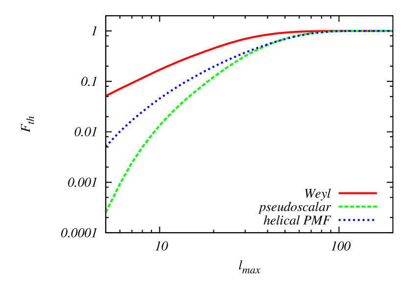
Figure 1: Signal-to-noise ratios of the parity-odd temperature bispectrum in the Weyl (red solid line), pseudoscalar (green dashed line) and helical PMF (blue dotted line) models, respectively. The values are normalized at max=200subscriptmax200\ell_{\rm max}=200.

Parity-odd signatures in the CMB bispectra [16, 18, 17] can arise when we consider Early Universe models including Chern-Simons like actions in Weyl gravity (f(ϕ)W~W2𝑓italic-ϕ~𝑊superscript𝑊2f(\phi)\widetilde{W}W^{2}) [8, 9] or inflationary models with rolling pseudoscalars (ϕF~Fitalic-ϕ~𝐹𝐹\phi\widetilde{F}F) [10, 12], or when we have primordial parity-odd objects, like helical primordial magnetic fields (PMFs) (see e.g., refs. [13, 14]). These signatures arise not from scalar, due to their spin-0 nature, but from tensor perturbations. Tensor-mode temperature signals are transferred to CMB temperature fluctuations via the Integrated Sachs-Wolfe (ISW) effect on large scales, while polarization signals appear on smaller scales due to Thomson scattering effects [27]. Accordingly, the temperature bispectra induced from the above NG sources can be large for 100less-than-or-similar-to100\ell\lesssim 100.

Figure 1 describes signal-to-noise ratios of the parity-odd temperature bispectra estimated for the three theoretical scenarios mentioned above (i.e., the so called Weyl, pseudoscalar and helical PMF models [16, 18, 17]) by mean of a brute force approach. The Fisher matrices for these models can be written, using the scalar product (3.10), as:

Fth=16v1v2v3b123(o)iC1C2C3,v1v2v3b123(o)iC1C2C3o.subscript𝐹th16subscriptexpectationsubscript𝑣subscript1subscript𝑣subscript2subscript𝑣subscript3superscriptsubscript𝑏subscript1subscript2subscript3𝑜𝑖subscript𝐶subscript1subscript𝐶subscript2subscript𝐶subscript3subscript𝑣subscript1subscript𝑣subscript2subscript𝑣subscript3superscriptsubscript𝑏subscript1subscript2subscript3𝑜𝑖subscript𝐶subscript1subscript𝐶subscript2subscript𝐶subscript3𝑜\displaystyle F_{\rm th}=\frac{1}{6}\Braket{\frac{v_{\ell_{1}}v_{\ell_{2}}v_{\ell_{3}}b_{\ell_{1}\ell_{2}\ell_{3}}^{(o)}}{i\sqrt{C_{\ell_{1}}C_{\ell_{2}}C_{\ell_{3}}}},\frac{v_{\ell_{1}}v_{\ell_{2}}v_{\ell_{3}}b_{\ell_{1}\ell_{2}\ell_{3}}^{(o)}}{i\sqrt{C_{\ell_{1}}C_{\ell_{2}}C_{\ell_{3}}}}}_{o}~{}. (4.1)

As shown in this figure, all the signal-to-noise ratios are saturated for max100greater-than-or-equivalent-tosubscriptmax100\ell_{\rm max}\gtrsim 100, due to the end of the ISW enhancement of the tensor mode.
Refer to caption Refer to caption
Refer to caption
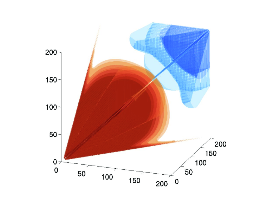
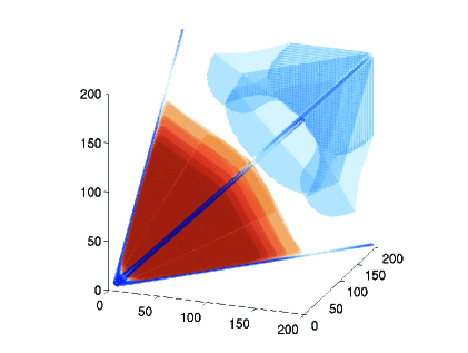
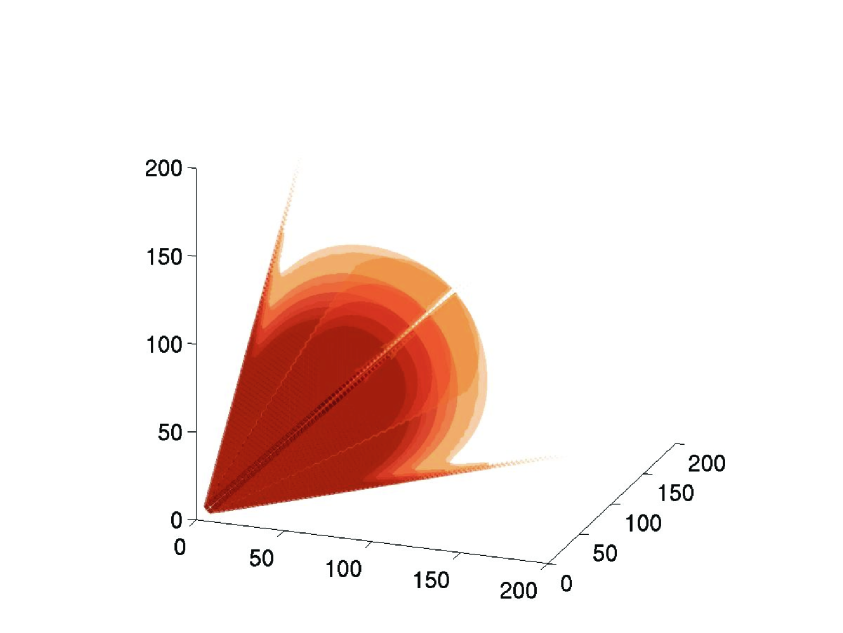
Figure 2: Three-dimensional representation of Weyl (left top panel), pseudoscalar (right top panel) and helical PMF (bottom panel) reduced bispectra in the tetrahedral domain (3.1). In order to remove an 4superscript4\ell^{-4} scaling, we rescale the shapes using a constant Sachs-Wolfe template [24].

Three-dimensional representations of these bispectra are described in figure 2. We can clearly see from the figure that the Weyl and pseudoscalar bispectra peak in the equilateral limit, while the helical PMF bispectrum peaks on the squeezed configurations. Note that these parity-odd bispectra vanish if two or three multipoles take the same values, i.e., B=B=B=0subscript𝐵subscript𝐵superscriptsubscript𝐵superscript0B_{\ell\ell\ell}=B_{\ell\ell\ell^{\prime}}=B_{\ell\ell^{\prime}\ell}=0.

In the following subsections, we will obtain modal decompositions for the three models above, and compare their performances to the brute-force approach. For safety and further accuracy, we will expand the bispectrum signals up to =200200\ell=200, although the signal-to-noise ratios almost converge for max100similar-tosubscriptmax100\ell_{\rm max}\sim 100. For convenience in the comparisons, we will fix the normalization of the bispectrum templates in such a way as to get Fth(max=200)=1subscript𝐹thsubscriptmax2001F_{\rm th}(\ell_{\rm max}=200)=1, as described in figure 1. 222These bispectrum amplitudes in the Weyl, pseudoscalar and helical PMF model are obtained when Λr2=1.1×10⁸Λsuperscript𝑟21.1superscript108\Lambda r^{-2}=1.1\times 10^{8} GeV, X=9.7×10⁵𝑋9.7superscript105X=9.7\times 10^{5} and 11/3B12/3=2.3superscriptsubscript113superscriptsubscript𝐵1232.3{\cal B}_{1}^{1/3}B_{1}^{2/3}=2.3 nG, respectively, where Λr2Λsuperscript𝑟2\Lambda r^{-2} is a combination of an energy scale of the dual cubic action and a tensor-to-scalar ratio in the Weyl gravity, X𝑋X is a coupling parameter of a pseudoscalar, and 11/3B12/3superscriptsubscript113superscriptsubscript𝐵123{\cal B}_{1}^{1/3}B_{1}^{2/3} is a combination of the helical and non-helical magnetic field strengths per 1 Mpc generated at the GUT epoch [16, 18, 17]. These parameter values will be detected at 68% CL through the parity-odd bispectrum estimation with noiseless large-scale (200less-than-or-similar-to200\ell\lesssim 200) data given by WMAP or Planck.

4.2 Modal decomposition

For (x,y,z)=(1,1,2)𝑥𝑦𝑧112(x,y,z)=(1,1,-2), γnpsubscript𝛾𝑛𝑝\gamma_{np} can explicitly written as

γnpsubscript𝛾𝑛𝑝\displaystyle\gamma_{np} =\displaystyle= 8π2311𝑑μζ{i{i1(o)1(ζjj1(o)1ζk}k}2(o)2+2ζjj2(o)1ζk}k}1(o)2)\displaystyle\frac{8\pi^{2}}{3}\int_{-1}^{1}d\mu~{}{}_{-1}\zeta_{\{i\{i^{\prime}1}^{(o)}\left({}_{-1}\zeta_{jj^{\prime}1}^{(o)}~{}{}_{2}\zeta_{k\}k^{\prime}\}-2}^{(o)}+2{}_{-1}\zeta_{jj^{\prime}-2}^{(o)}~{}{}_{2}\zeta_{k\}k^{\prime}\}1}^{(o)}\right) (4.2)
+16π2311𝑑μζ{i{i1(o)1(ζjj1(e)1ζk}k}2(e)2+ζjj2(e)1ζk}k}1(e)2)\displaystyle+\frac{16\pi^{2}}{3}\int_{-1}^{1}d\mu~{}{}_{-1}\zeta_{\{i\{i^{\prime}1}^{(o)}\left({}_{-1}\zeta_{jj^{\prime}1}^{(e)}~{}{}_{2}\zeta_{k\}k^{\prime}\}-2}^{(e)}+{}_{-1}\zeta_{jj^{\prime}-2}^{(e)}~{}{}_{2}\zeta_{k\}k^{\prime}\}1}^{(e)}\right)
+16π2311𝑑μ(ζ{i{i2(o)1ζjj1(e)1ζk}k}1(e)2+ζ{i{i1(o)2ζjj1(e)1ζk}k}2(e)1)\displaystyle+\frac{16\pi^{2}}{3}\int_{-1}^{1}d\mu\left({}_{-1}\zeta_{\{i\{i^{\prime}-2}^{(o)}~{}{}_{-1}\zeta_{jj^{\prime}1}^{(e)}~{}{}_{2}\zeta_{k\}k^{\prime}\}1}^{(e)}+{}_{2}\zeta_{\{i\{i^{\prime}1}^{(o)}~{}{}_{-1}\zeta_{jj^{\prime}1}^{(e)}~{}{}_{-1}\zeta_{k\}k^{\prime}\}-2}^{(e)}\right)
+8π2311𝑑μζ{i{i2(o)2ζjj1(e)1ζk}k}1(e)1.\displaystyle+\frac{8\pi^{2}}{3}\int_{-1}^{1}d\mu~{}{}_{2}\zeta_{\{i\{i^{\prime}-2}^{(o)}~{}{}_{-1}\zeta_{jj^{\prime}1}^{(e)}~{}{}_{-1}\zeta_{k\}k^{\prime}\}1}^{(e)}~{}.

Starting from this γ𝛾\gamma, we can calculate the expansion coefficients αnQsuperscriptsubscript𝛼𝑛𝑄\alpha_{n}^{Q} by use of eq. (3.8) and this γnpsubscript𝛾𝑛𝑝\gamma_{np}, and rotate to the orthonormal basis to get αnRsuperscriptsubscript𝛼𝑛𝑅\alpha_{n}^{R}. We implemented a stable numerical algorithm that perform these operations using about 200200200 modes in 555 CPU hours.

Refer to caption
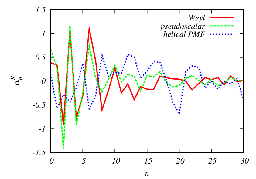
Figure 3: Modal coefficients in the orthonormal basis, αnRsuperscriptsubscript𝛼𝑛𝑅\alpha_{n}^{R}, in the Weyl (red solid line), pseudoscalar (green dashed line) and helical PMF (blue dotted line) models, respectively. Here we decompose with the polynomial eigenfunctions and an additional function (n=1𝑛1n=1) sensitive to the squeezed-limit signals.

Figure 3 depicts the spectrum of mode coefficients as a function of mode number each n𝑛n. We plot as usual the αRsuperscript𝛼𝑅\alpha^{R} coefficients, related to the orthonormal expansion. The interpretation of the results in the rotated space is in fact more straightforward due to the fact that, as a consequence of orthonormality of the basis templates, the expansion coefficients are uncorrelated. Here, we have decomposed using an hybrid basis involving polynomial eigenfunctions and a special mode function enhanced at the squeezed limit (this is the same basis used for the analysis of Planck data [5] using the parity-even pipeline; here we use however a smaller number of modes, since we work at lower maxsubscriptmax\ell_{\rm max}, which allows for more rapid convergence). In the chosen mode ordering, the squeezed mode is located at n=1𝑛1n=1. In the helical PMF case, the n=1𝑛1n=1 mode is relatively large compared with the other modes due to the squeezed-limit amplification, while, as expected, it is not prominent in the equilateral-type bispectra in the Weyl and pseudoscalar cases. We find that αnRsuperscriptsubscript𝛼𝑛𝑅\alpha_{n}^{R}’s in these equilateral bispectra converge more rapidly compared with the squeezed-type one.
Refer to caption
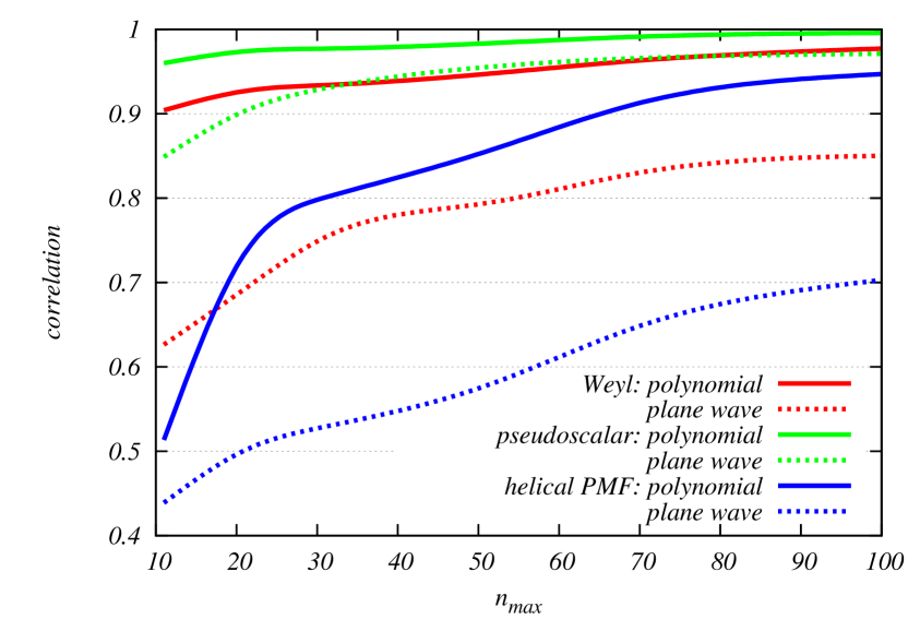
Figure 4: Correlations between exact bispectra and modal-decomposed ones up to nmaxsubscript𝑛maxn_{\rm max}, in the Weyl (red lines), pseudoscalar (green lines) and helical PMF (blue lines) models, respectively. Here, we compare the differences in convergence between the polynomial + squeezed mode (solid lines) and the plane-wave + squeezed mode (dotted lines) decompositions.

The convergence of the expansion is assessed via computation of the correlation between the full starting theoretical bispectrum and the modal-decomposed one. Using the orthonormal basis expansion, it is easy to verify that the correlation between the two is expressed as FthR/FthFRsubscript𝐹th𝑅subscript𝐹thsubscript𝐹𝑅F_{{\rm th}R}/\sqrt{F_{\rm th}F_{R}}, where each Fisher matrix is given by eq. (4.1) and

FthRsubscript𝐹th𝑅\displaystyle F_{{\rm th}R} =\displaystyle= 16v1v2v3b123(o)iC1C2C3,n=0nmaxαnRRn(1,2,3)o,16subscriptexpectationsubscript𝑣subscript1subscript𝑣subscript2subscript𝑣subscript3superscriptsubscript𝑏subscript1subscript2subscript3𝑜𝑖subscript𝐶subscript1subscript𝐶subscript2subscript𝐶subscript3superscriptsubscript𝑛0subscript𝑛maxsuperscriptsubscript𝛼𝑛𝑅subscript𝑅𝑛subscript1subscript2subscript3𝑜\displaystyle\frac{1}{6}\Braket{\frac{v_{\ell_{1}}v_{\ell_{2}}v_{\ell_{3}}b_{\ell_{1}\ell_{2}\ell_{3}}^{(o)}}{i\sqrt{C_{\ell_{1}}C_{\ell_{2}}C_{\ell_{3}}}},\sum_{n=0}^{n_{\rm max}}\alpha_{n}^{R}R_{n}(\ell_{1},\ell_{2},\ell_{3})}_{o}~{}, (4.3)
FRsubscript𝐹𝑅\displaystyle F_{R} =\displaystyle= 16n=0nmax(αnR)2.16superscriptsubscript𝑛0subscript𝑛maxsuperscriptsuperscriptsubscript𝛼𝑛𝑅2\displaystyle\frac{1}{6}\sum_{n=0}^{n_{\rm max}}(\alpha_{n}^{R})^{2}~{}. (4.4)

Figure 4 shows numerical results of the correlations obtained from the modal decompositions as a function of nmaxsubscript𝑛maxn_{\rm max}, where nmaxsubscript𝑛maxn_{\rm max} denotes the number of modes at which we truncate our numerical expansions. For this analysis, we have adopted both the hybrid polynomial-squeezed basis described above and an additional plane-wave decomposition, also equipped with the n=1𝑛1n=1 squeezed mode. Like the polynomial basis, also the plane-wave expansion was already adopted in the context of WMAP and Planck data analysis for parity-even bispectra. From the figure we can observe that, in all three models, the polynomial decompositions achieve more than 90% correlations already for nmax70greater-than-or-equivalent-tosubscript𝑛max70n_{\rm max}\gtrsim 70, while the plane-wave decomposed bispectra are less correlated with the theoretical templetes than the polynomial ones. The convergence speed seems to depend strongly on the bispectrum shape. The polynomial basis can reconstruct the pseudoscalar bispectrum more rapidly, achieving 98% correlation for nmax40similar-to-or-equalssubscript𝑛max40n_{\rm max}\simeq 40. In another equilateral-type case, namely the Weyl model, the convergence is a bit weaker and the correlation reaches around 0.98 for nmax100similar-to-or-equalssubscript𝑛max100n_{\rm max}\simeq 100. For the squeezed-type helical PMF model the convergence is even slower, but we can still get the correlation to exceed 0.98 for nmax200greater-than-or-equivalent-tosubscript𝑛max200n_{\rm max}\gtrsim 200. A similar tendency can be seen in the plane-wave decompositions, but the values of correlations drop overall. So we can conclude that for these templates a polynomial decomposition is more efficient than a plane-wave one.

4.3 Non-Gaussian map simulation

We now discuss the issue of simulation of NG maps including bispectra from each of our three theoretical models. The NG part of the map multipoles can be written in separable form for (x,y,z)=(1,1,2)𝑥𝑦𝑧112(x,y,z)=(1,1,-2), in the following way

amNG{amNGoo+amNGee(=odd)amNGoe+amNGeo(=even),superscriptsubscript𝑎𝑚NGcasessuperscriptsubscript𝑎𝑚NG𝑜𝑜superscriptsubscript𝑎𝑚NG𝑒𝑒oddsuperscriptsubscript𝑎𝑚NG𝑜𝑒superscriptsubscript𝑎𝑚NG𝑒𝑜even\displaystyle a_{\ell m}^{\rm NG}\equiv\begin{cases}a_{\ell m}^{{\rm NG}oo}+a_{\ell m}^{{\rm NG}ee}&(\ell={\rm odd})\\ a_{\ell m}^{{\rm NG}oe}+a_{\ell m}^{{\rm NG}eo}&(\ell={\rm even})\end{cases}~{}, (4.5)

where

amNGabsuperscriptsubscript𝑎𝑚NG𝑎𝑏\displaystyle a_{\ell m}^{{\rm NG}ab} =\displaystyle= iC54vnijkαnQd2𝐧^𝑖subscript𝐶54subscript𝑣subscript𝑛𝑖𝑗𝑘superscriptsubscript𝛼𝑛𝑄superscript𝑑2^𝐧\displaystyle\frac{i\sqrt{C_{\ell}}}{54v_{\ell}}\sum_{n\leftrightarrow ijk}\alpha_{n}^{Q}\int d^{2}\hat{\bf n} (4.6)
×[qi()Ym1(MjG(a)1MkG(b)2+MjG(a)2MkG(b)1)\displaystyle\times\left[q_{i}(\ell){}_{-1}Y_{\ell m}\left({}_{-1}M_{j}^{{\rm G}(a)}~{}{}_{2}M_{k}^{{\rm G}(b)}+{}_{2}M_{j}^{{\rm G}(a)}~{}{}_{-1}M_{k}^{{\rm G}(b)}\right)\right.
+qi()Ym2MjG(a)1MkG(b)1subscript𝑞𝑖subscriptsubscript𝑌𝑚2subscriptsuperscriptsubscript𝑀𝑗G𝑎1subscriptsuperscriptsubscript𝑀𝑘G𝑏1\displaystyle\left.\quad+q_{i}(\ell){}_{2}Y_{\ell m}~{}{}_{-1}M_{j}^{{\rm G}(a)}~{}{}_{-1}M_{k}^{{\rm G}(b)}\right.
+qj()Ym1(MkG(a)1MiG(b)2+MkG(a)2MiG(b)1)subscript𝑞𝑗subscriptsubscript𝑌𝑚1subscriptsuperscriptsubscript𝑀𝑘G𝑎1subscriptsuperscriptsubscript𝑀𝑖G𝑏2subscriptsuperscriptsubscript𝑀𝑘G𝑎2subscriptsuperscriptsubscript𝑀𝑖G𝑏1\displaystyle\left.\quad+q_{j}(\ell){}_{-1}Y_{\ell m}\left({}_{-1}M_{k}^{{\rm G}(a)}~{}{}_{2}M_{i}^{{\rm G}(b)}+{}_{2}M_{k}^{{\rm G}(a)}~{}{}_{-1}M_{i}^{{\rm G}(b)}\right)\right.
+qj()Ym2MkG(a)1MiG(b)1subscript𝑞𝑗subscriptsubscript𝑌𝑚2subscriptsuperscriptsubscript𝑀𝑘G𝑎1subscriptsuperscriptsubscript𝑀𝑖G𝑏1\displaystyle\left.\quad+q_{j}(\ell){}_{2}Y_{\ell m}~{}{}_{-1}M_{k}^{{\rm G}(a)}~{}{}_{-1}M_{i}^{{\rm G}(b)}\right.
+qk()Ym1(MiG(a)1MjG(b)2+MiG(a)2MjG(b)1)subscript𝑞𝑘subscriptsubscript𝑌𝑚1subscriptsuperscriptsubscript𝑀𝑖G𝑎1subscriptsuperscriptsubscript𝑀𝑗G𝑏2subscriptsuperscriptsubscript𝑀𝑖G𝑎2subscriptsuperscriptsubscript𝑀𝑗G𝑏1\displaystyle\left.\quad+q_{k}(\ell){}_{-1}Y_{\ell m}\left({}_{-1}M_{i}^{{\rm G}(a)}~{}{}_{2}M_{j}^{{\rm G}(b)}+{}_{2}M_{i}^{{\rm G}(a)}~{}{}_{-1}M_{j}^{{\rm G}(b)}\right)\right.
+qk()Ym2MiG(a)1MjG(b)1],\displaystyle\left.\quad+q_{k}(\ell){}_{2}Y_{\ell m}~{}{}_{-1}M_{i}^{{\rm G}(a)}~{}{}_{-1}M_{j}^{{\rm G}(b)}\right]^{*}~{},

with a,bo,eformulae-sequence𝑎𝑏𝑜𝑒a,b\in o,e.

Refer to caption
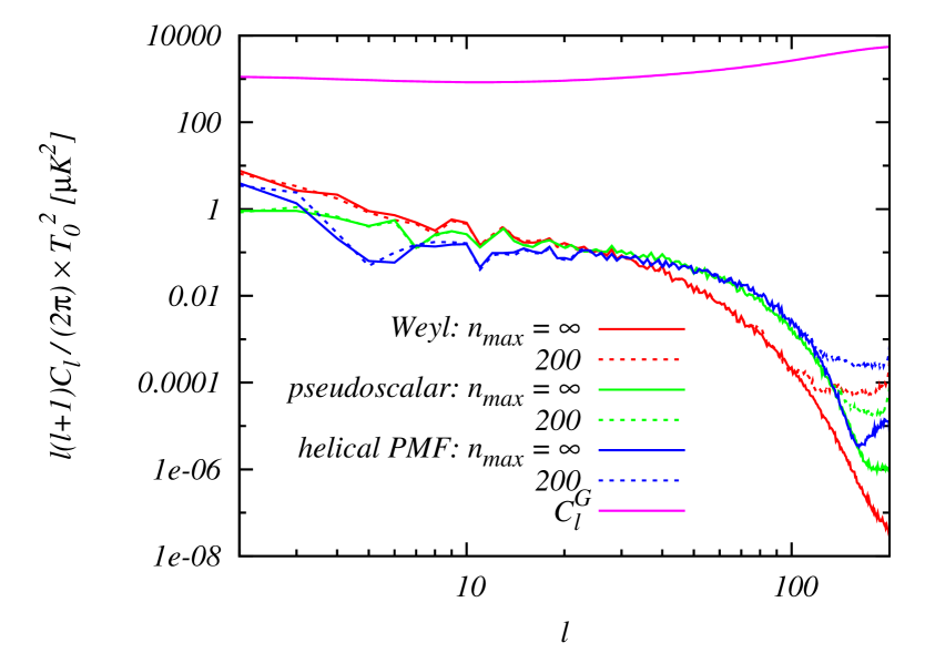
Figure 5: Power spectra of amGsuperscriptsubscript𝑎𝑚Ga_{\ell m}^{\rm G}’s in the Weyl (red lines), pseudoscalar (green lines) and helical PMF (blue lines) models, respectively. Here, for comparison of convergence, we plot the exact results, namely nmax=subscript𝑛maxn_{\rm max}=\infty, estimated in the direct non-separable computations (solid lines), and the results obtained in the nmax=200subscript𝑛max200n_{\rm max}=200 modal decompositions (dotted lines). CGsuperscriptsubscript𝐶GC_{\ell}^{\rm G} denotes the Gaussian part of Csubscript𝐶C_{\ell}.

Figure 5 describes the power spectrum of amNGsuperscriptsubscript𝑎𝑚NGa_{\ell m}^{\rm NG} in each theoretical model. Here we can compare the results from the separable modal decompositions for nmax=200subscript𝑛max200n_{\rm max}=200 given by eq. (4.5) with the exact results from direct non-separable computations of eq. (1.7), which should be equivalent to the nmax=subscript𝑛maxn_{\rm max}=\infty modal decomposition. As expected, we find that, with pre-computed modal coefficients α𝛼\alpha, the separable modal approach drastically reduces the CPU time from 120 to 0.2 CPU hours. From figure 5, it is also clear that the modal results are in good agreement with the exact non-separable computation up to 100similar-to-or-equals100\ell\simeq 100 in all three models. This comes from the fact that, for nmax=200subscript𝑛max200n_{\rm max}=200, the modal bispectrum reconstructs the exact shape with more than 98% correlation in each model. In contrast, for 100greater-than-or-equivalent-to100\ell\gtrsim 100, the modal results tend to deviate from the exact ones. This is due to numerical instabilities in the computation of MiG(o/e)xsubscriptsuperscriptsubscript𝑀𝑖G𝑜𝑒𝑥{}_{x}M_{i}^{{\rm G}(o/e)}, and of the angular integrals of their products. We found that this issue can be circumvented by expanding the bispectra and generating maps with an angular resolution much larger than the required maxsubscriptmax\ell_{\rm max} for the analyis, and then smoothing the maps by picking only multipoles up to maxsubscript𝑚𝑎𝑥\ell_{max}. Concerning the shapes that are specifically under study, all three spectra decay for >100100\ell>100 due to the end of the tensor-mode ISW enhancement, so this approach is not unfeasible.

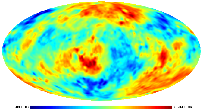
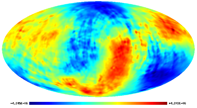
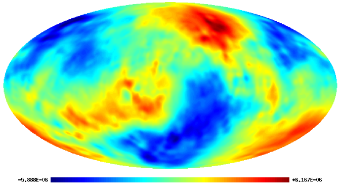
Figure 6 shows the NG part of a simulated map for each of the three models we are testing; the three maps have been obtained starting from the same Gaussian seed, and we have considered multipoles up to =100100\ell=100, in order to avoid the numerical instabilities mentioned above.
Refer to caption
Refer to caption
Refer to caption
Figure 6: Simulated parity-odd NG CMB maps [kelvin] from the Weyl (top panel), pseudoscalar (middle panel) and helical PMF (bottom panel) models, respectively. The maps are generated from amNGsuperscriptsubscript𝑎𝑚NGa_{\ell m}^{\rm NG}’s up to =100100\ell=100, whose power spectra are depicted in figure 5.

5 Conclusion

Despite the fact that there are several theoretical primordial scenarios predicting the existence of parity-odd bispectra, no observational constraint on this type of NG has been placed so far. Generally, parity-odd bispectra are written in non-separable form, and this has made data analysis unpractical, due to large CPU-time requirements. This paper has developed a new framework for parity-odd CMB bispectrum estimation by extending the separable modal decomposition methodology, already developed and used for parity-even analyses, to parity-odd domains. The analytical extension to the case of interest has been obtained by defining a new reduced bispectrum and a new inner product weight function, in such a way as to account for spin dependence, and to change selection rules in order to include 1+2+3=oddsubscript1subscript2subscript3odd\ell_{1}+\ell_{2}+\ell_{3}={\rm odd} configurations. In this way, we can achieve separability of parity-odd NG estimators and get fast NG maps algorithm, in strict analogy to the parity-even modal expansion procedure.

Our parity-odd modal decomposition has been numerically implemented and tested by expanding temperature bispectra predicted by several parity-odd Early Universe models. We have checked that the numerical algorithm is stable and achieves convergence using a reasonable number of templates in a few CPU-hours. The exact convergence efficiency depends on the bispectrum shape and the type of modal eigenfunctions. Using decomposed separable bispectra, we have also produced NG simulations and checked the consistency with the exact results from a slow brute-force approach. As expected, we get massive computational gains when working with separable modal bispectra.

The algorithm for bispectrum estimation developed in this paper is applicable to all types of parity-odd bispectra (i.e., bispectra enforcing the condition 1+2+3=oddsubscript1subscript2subscript3odd\ell_{1}+\ell_{2}+\ell_{3}={\rm odd}). Our numerical approach so far has included only temperature bispectra. Future interesting applications will include actual estimation of parity-odd NG from CMB data, and the extension of our method to polarized bispectra, which are generally predicted in parity-odd scenarios, with taking care of bias due to the experimental systematics or the imperfect sky coverage.

Acknowledgments

We are very grateful to Paul Shellard for many useful discussions. MS is supported in part by a Grant-in-Aid for JSPS Research under Grant No. 25-573. This work is supported in part by the ASI/INAF Agreement I/072/09/0 for the Planck LFI Activity of Phase E2.

References

  • [1] V. Acquaviva, N. Bartolo, S. Matarrese, and A. Riotto, Second order cosmological perturbations from inflation, Nucl.Phys. B667 (2003) 119–148, [astro-ph/0209156].
  • [2] J. M. Maldacena, Non-Gaussian features of primordial fluctuations in single field inflationary models, JHEP 0305 (2003) 013, [astro-ph/0210603].
  • [3] N. Bartolo, E. Komatsu, S. Matarrese, and A. Riotto, Non-Gaussianity from inflation: Theory and observations, Phys.Rept. 402 (2004) 103–266, [astro-ph/0406398].
  • [4] E. Komatsu, Hunting for Primordial Non-Gaussianity in the Cosmic Microwave Background, Class. Quant. Grav. 27 (2010) 124010, [arXiv:1003.6097].
  • [5] Planck Collaboration Collaboration, P. Ade et. al., Planck 2013 Results. XXIV. Constraints on primordial non-Gaussianity, arXiv:1303.5084.
  • [6] D. Babich and M. Zaldarriaga, Primordial bispectrum information from CMB polarization, Phys.Rev. D70 (2004) 083005, [astro-ph/0408455].
  • [7] A. P. Yadav, E. Komatsu, and B. D. Wandelt, Fast Estimator of Primordial Non-Gaussianity from Temperature and Polarization Anisotropies in the Cosmic Microwave Background, Astrophys.J. 664 (2007) 680–686, [astro-ph/0701921].
  • [8] J. M. Maldacena and G. L. Pimentel, On graviton non-Gaussianities during inflation, JHEP 1109 (2011) 045, [arXiv:1104.2846].
  • [9] J. Soda, H. Kodama, and M. Nozawa, Parity Violation in Graviton Non-gaussianity, JHEP 1108 (2011) 067, [arXiv:1106.3228].
  • [10] N. Barnaby, J. Moxon, R. Namba, M. Peloso, G. Shiu, et. al., Gravity waves and non-Gaussian features from particle production in a sector gravitationally coupled to the inflaton, Phys.Rev. D86 (2012) 103508, [arXiv:1206.6117].
  • [11] T. Zhu, W. Zhao, Y. Huang, A. Wang, and Q. Wu, Effects of parity violation on non-gaussianity of primordial gravitational waves in Hořava-Lifshitz gravity, Phys.Rev. D88 (2013) 063508, [arXiv:1305.0600].
  • [12] J. L. Cook and L. Sorbo, An inflationary model with small scalar and large tensor nongaussianities, JCAP 1311 (2013) 047, [arXiv:1307.7077].
  • [13] C. Caprini, R. Durrer, and T. Kahniashvili, The Cosmic microwave background and helical magnetic fields: The Tensor mode, Phys.Rev. D69 (2004) 063006, [astro-ph/0304556].
  • [14] T. Kahniashvili and B. Ratra, Effects of Cosmological Magnetic Helicity on the Cosmic Microwave Background, Phys.Rev. D71 (2005) 103006, [astro-ph/0503709].
  • [15] M. Kamionkowski and T. Souradeep, The Odd-Parity CMB Bispectrum, Phys.Rev. D83 (2011) 027301, [arXiv:1010.4304].
  • [16] M. Shiraishi, D. Nitta, and S. Yokoyama, Parity Violation of Gravitons in the CMB Bispectrum, Prog.Theor.Phys. 126 (2011) 937–959, [arXiv:1108.0175].
  • [17] M. Shiraishi, Parity violation of primordial magnetic fields in the CMB bispectrum, JCAP 1206 (2012) 015, [arXiv:1202.2847].
  • [18] M. Shiraishi, A. Ricciardone, and S. Saga, Parity violation in the CMB bispectrum by a rolling pseudoscalar, JCAP 1311 (2013) 051, [arXiv:1308.6769].
  • [19] M. Shiraishi, Polarization bispectrum for measuring primordial magnetic fields, JCAP 1311 (2013) 006, [arXiv:1308.2531].
  • [20] A. Lewis, A. Challinor, and D. Hanson, The shape of the CMB lensing bispectrum, JCAP 1103 (2011) 018, [arXiv:1101.2234].
  • [21] WMAP Collaboration Collaboration, E. Komatsu et. al., Five-Year Wilkinson Microwave Anisotropy Probe (WMAP) Observations: Cosmological Interpretation, Astrophys.J.Suppl. 180 (2009) 330–376, [arXiv:0803.0547].
  • [22] K. M. Smith and M. Zaldarriaga, Algorithms for bispectra: Forecasting, optimal analysis, and simulation, Mon.Not.Roy.Astron.Soc. 417 (2011) 2–19, [astro-ph/0612571].
  • [23] E. Komatsu, D. N. Spergel, and B. D. Wandelt, Measuring primordial non-Gaussianity in the cosmic microwave background, Astrophys.J. 634 (2005) 14–19, [astro-ph/0305189].
  • [24] J. Fergusson, M. Liguori, and E. Shellard, General CMB and Primordial Bispectrum Estimation I: Mode Expansion, Map-Making and Measures of FNLsubscript𝐹NLF_{\rm NL}, Phys.Rev. D82 (2010) 023502, [arXiv:0912.5516].
  • [25] J. Fergusson, M. Liguori, and E. Shellard, The CMB Bispectrum, JCAP 1212 (2012) 032, [arXiv:1006.1642].
  • [26] J. R. Fergusson and E. P. S. Shellard, Optimal Polyspectra Estimation, arXiv:1105.2791.
  • [27] J. R. Pritchard and M. Kamionkowski, Cosmic microwave background fluctuations from gravitational waves: An Analytic approach, Annals Phys. 318 (2005) 2–36, [astro-ph/0412581].