Galaxy Shapes and Intrinsic Alignments in the MassiveBlack-II Simulation

Abstract

The intrinsic alignment of galaxy shapes with the large-scale density field is a contaminant to weak lensing measurements, as well as being an interesting signature of galaxy formation and evolution (albeit one that is difficult to predict theoretically). Here we investigate the shapes and relative orientations of the stars and dark matter of halos and subhalos (central and satellite) extracted from the MassiveBlack-II simulation, a state-of-the-art high resolution hydrodynamical cosmological simulation which includes stellar and AGN feedback in a volume of $(100$$h^{-1}\mathrm{Mpc}$$)^{3}$. We consider redshift evolution from $z=1$ to $0.06$ and mass evolution within the range of subhalo masses, $10^{10}-6.0\times 10^{14.0}$$h^{-1}M_{\odot}$. The shapes of the dark matter distributions are generally more round than the shapes defined by stellar matter. The projected root-mean-square (RMS) ellipticity per component for stellar matter is measured to be $e_{\text{rms}}=0.28$ at $z=0.3$ for $M_{\text{subhalo}}>10^{12.0}$$h^{-1}M_{\odot}$, which compares favourably with observational measurements. We find that the shapes of stellar and dark matter are more round for less massive subhalos and at lower redshifts. By directly measuring the relative orientation of the stellar matter and dark matter of subgroups, we find that, on average, the misalignment between the two components is larger for less massive subhalos. The mean misalignment angle varies from $\sim 30^{\circ}-10^{\circ}$ for $M\sim 10^{10}-10^{14}h^{-1}M_{\odot}$ and shows a weak dependence on redshift. We also compare the misalignment angles in central and satellite subhalos at fixed subhalo mass, and find that centrals are more misaligned than satellites. We present fitting formulae for the shapes of dark and stellar matter in subhalos and also the probability distributions of misalignment angles.

1 Introduction

Weak gravitational lensing is a useful probe to constrain cosmological parameters since it is sensitive to both luminous and dark matter (Hu, 2002; Benabed & van Waerbeke, 2004; Ishak et al., 2004; Takada & White, 2004; Bernstein & Jain, 2004; Huterer, 2010). In particular, weak lensing surveys can be used to probe theories of modified gravity and provide constraints on the properties of dark matter and dark energy (Albrecht et al., 2006; Weinberg et al., 2013). Many upcoming surveys like Large Synoptic Survey Telescope(LSST) and Euclid aim to determine the constant and dynamical parameters of the dark energy equation of state to a very high precision using weak lensing.

However, constraining cosmological parameters with sub-percent errors in future cosmological survey requires the systematic errors to be well below those in typical weak lensing measurements with current datasets. The intrinsic shapes and orientations of galaxies are not random but correlated with each other and the underlying density field. This is known as intrinsic galaxy alignments. The intrinsic alignment (IA) of galaxy shapes with the underlying density field is an important theoretical uncertainty that contaminates weak lensing measurements (Heavens et al., 2000; Croft & Metzler, 2000; Jing, 2002; Hirata & Seljak, 2004). Accurate theoretical predictions of IA through analytical models and $N$-body simulations (Hirata & Seljak, 2004; Heymans et al., 2006; Schneider & Bridle, 2010; Joachimi et al., 2013) in the $\Lambda$CDM paradigm is complicated by the absence of baryonic physics, which we expect to be important given that the alignment of interest is that of the observed, baryonic component of galaxies. So, we either need simulations that include the physics of galaxy formation or $N$-body simulations with rules for galaxy shapes and alignments.

Proposed analysis methods to remove IA from weak lensing measurements either involve removing considerable amount of cosmological information (which requires very accurate redshift information; nulling methods: Joachimi & Schneider 2008, 2009), or involve marginalizing over parametrized models of how the intrinsic alignments affect observations as a function of scale, redshift and galaxy type (e.g., Bridle & King, 2007; Joachimi & Bridle, 2010; Blazek et al., 2012). The simultaneous fitting method, with a relatively simple intrinsic alignments model, was used for a tomographic cosmic shear analysis of CFHTLenS data (Heymans et al., 2013). The latter methods, while preserving more cosmological information than nulling methods, can only work correctly if there is a well-motivated intrinsic alignments model as a function of galaxy properties. Existing candidates for the intrinsic alignment model to be used in such an approach include the linear alignment model (Hirata & Seljak, 2004) or simple modifications of it (e.g., using the nonlinear power spectrum: Bridle & King 2007), $N$-body simulations populated with galaxies and stochastically misaligned with halos in a way that depends on galaxy type (Heymans et al., 2006), and the halo model (Schneider & Bridle, 2010), which includes rules for how central and satellite galaxies are intrinsically aligned.

In this study, we use the large volume, high-resolution hydrodynamic simulation, MassiveBlack-II (Khandai et al., 2014), which includes a range of baryonic processes to directly study the shapes and alignments of galaxies. In particular, we measure directly the shapes of the dark and stellar matter components of halos and subhalos (modeled as ellipsoids in three dimensional space). We examine how shapes evolve with time and as a function of halo/subhalo mass. Previous work used $N$-body simulations and analytical modeling to study triaxial shape distributions of dark matter halos as a function of mass and their evolution with redshift (Hopkins et al., 2005; Allgood et al., 2006; Lee et al., 2005; Schneider et al., 2012). More recently, hydrodynamic cosmological simulations have also been used to study the effects of baryonic physics on the shapes of dark matter halos (Bailin et al., 2005; Kazantzidis et al., 2006; Knebe et al., 2010; Bryan et al., 2013). Here, using a high-resolution hydrodynamic simulation in a large cosmological volume that incorporates the physics of star formation and associated feedback as well as black hole accretion and AGN feedback, we focus on measuring directly the shapes of the stellar components of galaxies and examine the misalignments between stars and dark matter in galaxies (central and satellite). We also measure the projected (2D) shapes for comparison with observations. This study is important because the measured intrinsic alignments of galaxies are related to the projected shape correlations of the stellar component of subgroups (galaxies) by the density-ellipticity and ellipticity-ellipticity correlations (Heymans et al., 2006). By measuring the projected ellipticities of the stellar and dark matter component of simulated galaxies, we can attempt to understand the differences between these two. In addition, we can do a basic comparison of the stellar components with observational results, and validate the realism of the simulated galaxy population.

Another aspect of the problem that we consider in this paper is the relative orientation of the stellar component of the halo with its dark matter component. Many dark matter-only simulations have illustrated that dark matter halos exhibit large-scale intrinsic alignments (e.g., Faltenbacher et al., 2002; Hopkins et al., 2005; Altay et al., 2006; Heymans et al., 2006), but the prediction of galaxy intrinsic alignments from halo intrinsic alignments requires a statistical understanding of the relationship between galaxy and halo shapes. To date, there has been no direct measurement of galaxy versus halo misalignment with a large statistical sample of galaxies through hydrodynamic simulations. Recently, Dubois et al. (2014) studied the alignment between the spin of galaxies and their host filament direction using a hydrodynamical cosmological simulation of box size $100h^{-1}\mathrm{Mpc}$. Studies of misalignment based on SPH simulations of smaller volumes detected misalignments between the baryonic and dark matter component of halos (van den Bosch et al., 2003; Sharma & Steinmetz, 2005; Hahn et al., 2010; Deason et al., 2011). These studies considered the correlation of spin and angular momentum of the baryonic component with dark matter. The spin correlations are arguably more relevant for the intrinsic alignments of spiral galaxies (Hirata & Seljak, 2004), whereas the observed intrinsic alignments in real galaxy samples are dominated by red, pressure-supported, elliptical galaxies (Mandelbaum et al., 2011; Joachimi et al., 2011); hence a study of the correlation of projected shapes is more relevant for the issue of weak lensing contamination. However, to make precise predictions based on the halo or subhalo mass at different redshifts, we need a hydrodynamic simulation of very large volume and high resolution. The MassiveBlack-II SPH simulation meets those requirements, making it a good choice for this kind of study.

Others arrived at constraints on misalignments using $N$-body simulations and calibrating the misalignments by adopting a simple parametric form to agree with observationally detected shape correlation functions (Faltenbacher et al., 2009; Okumura et al., 2009). There are also studies of the alignment of a central galaxy with its host halo where it is assumed that the satellites trace the dark matter distribution (e.g., Wang et al., 2008). By using hydrodynamic simulations, we can directly calculate the misalignment distributions for all galaxies as a function of halo mass and cosmic time. Resolution of the galaxies into centrals and satellites also helps to understand the effect of local environment.

This paper is organized as follows. In Section 2, we describe the SPH simulations used for this work and the methods used to obtain the shapes and orientations of groups and subgroups. In Section 3, we give the axis ratio distributions of dark matter and stellar matter of subgroups. In Section 4, we show our results for misalignments of the stellar component of subgroups with their host dark matter subgroups. In Section 5 we compare the shape distributions and misalignment angle between centrals and satellites. Finally, we summarize our conclusions in Section 6. The functional forms for our results are provided in the Appendix.

2 Methods

2.1 MassiveBlack-II Simulation

$\begin{array}[]{c@{\hspace{0.1in}}c}\includegraphics[width=433.62pt,angle={0}]{lss_1113_new}\hfil\hskip 7.22743pt\\ \includegraphics[width=166.2212pt,height=166.2212pt,angle={0}]{mg_0_1113}\ \includegraphics[width=166.2212pt,height=166.2212pt,angle={0}]{mg_989_1113}\ \includegraphics[width=166.2212pt,height=166.2212pt,angle={0}]{mg_3000_1113}\hfil\hskip 7.22743pt\\ \end{array}$

Figure 1: Top: Snapshot of the MBII simulation in a slice of thickness $2$$h^{-1}\mathrm{Mpc}$ at redshift $z=0.06$. The bluish-white colored region represents the density of the dark matter distribution and the red lines show the direction of the major axis of ellipse for the projected shape defined by the stellar component. Bottom Left: Dark matter (shown in gray) and stellar matter (shown in red) distribution in the most massive group at $z=0.06$ of mass $7.2\times 10^{14}$$h^{-1}M_{\odot}$. The blue and red ellipses show the projected shapes of dark matter and stellar matter of subhalos respectively. Bottom Middle: Dark matter and stellar matter distribution in a group of mass $3.8\times 10^{12}$$h^{-1}M_{\odot}$. Bottom Right: Dark matter and stellar matter distribution in a group of mass $1.1\times 10^{12}$$h^{-1}M_{\odot}$.

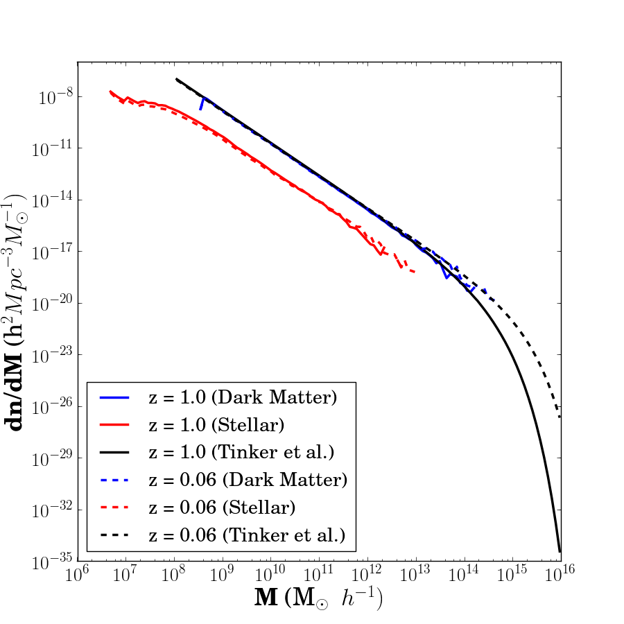
Figure 2: Dark matter and stellar mass function for FOF groups (halos) at $z=0.06,1.0$, compared with the SO-based prediction from Tinker et al. (2008) generated with $\Delta=0.75$.

We use the MassiveBlack-II (MBII) simulation to measure shapes and alignments of dark matter and stellar components of halos and subhalos. MBII is a state-of-the-art high resolution, large volume, cosmological hydrodynamic simulation of structure formation. An extensive description of the simulation and major predictions for the halo and subhalo mass functions, their clustering, the galaxy stellar mass functions, galaxy spectral energy distribution and properties of the AGN population is presented by Khandai et al. (2014). We refer the reader to this publication for details on MBII and briefly summarize the major relevant aspects here.

The MBII simulation was performed with the cosmological TreePM-Smooth Particle Hydrodynamics (SPH) code p-gadget. It is a hybrid version of the parallel code, gadget2 (Springel et al., 2005a) that has been upgraded to run on Petaflop scale supercomputers. In addition to gravity and SPH, the p-gadget code also includes the physics of multi-phase ISM model with star formation (Springel & Hernquist, 2003a), black hole accretion and feedback (Springel et al., 2005a; Di Matteo et al., 2012). Radiative cooling and heating processes are included (as in Katz et al., 1996), as is photoheating due to an imposed ionizing UV background. The interstellar medium (ISM), star formation and supernovae feedback as well as black hole accretion and associated feedback are treated by means of previously developed sub-resolution models. In particular, the multiphase model for star forming gas we use, developed by Springel & Hernquist (2003b), has two principal ingredients: (1) a star formation prescription and (2) an effective equation of state (EOS). A thermal instability is assumed to operate above a critical density threshold $\rho_{\rm th}$, producing a two phase medium consisting of cold clouds embedded in a tenuous gas at pressure equilibrium. Stars form from the cold clouds, and short-lived stars supply an energy of $10^{51}\,{\rm ergs}$ to the surrounding gas as supernovae. This energy heats the diffuse phase of the ISM and evaporates cold clouds, thereby establishing a self-regulation cycle for star formation. $\rho_{\rm th}$ is determined self-consistently in the model by requiring that the EOS is continuous at the onset of star formation. Stellar feedback in the form of stellar winds is also included. The prescription for black hole accretion and associated feedback from massive black holes follows the one developed by  Di Matteo et al. (2005); Springel et al. (2005b). We represent black holes by collisionless particles that grow in mass by accreting gas (at the local dynamical timescale) from their environments. If the accretion rates reach the critical Eddington limit they are then capped at that value. A fraction $f$ (fixed to $5\%$ to fit the local black-hole galaxy relations) of the radiative energy released by the accreted material is assumed to couple thermally to nearby gas and influence its thermodynamic state. Black holes merge when they approach the spatial resolution limit of the simulation (Springel & Hernquist, 2003b)

MBII contains $N_{\mathrm{part}}=2\times 1792^{3}$ dark matter and gas particles in a cubic periodic box of length $100$$h^{-1}\mathrm{Mpc}$ on a side, with a gravitational smoothing length $\epsilon=1.85$$h^{-1}\mathrm{kpc}$ in comoving units. A single dark matter particle has a mass $m_{DM}=1.1\times 10^{7}h^{-1}M_{\odot}$ and the initial mass of a gas particle is $m_{gas}=2.2\times 10^{6}h^{-1}M_{\odot}$. The cosmological parameters used in the simulation are as follows: amplitude of matter fluctuations $\sigma_{8}=0.816$, spectral index $\eta_{s}=0.96$, mass density parameter $\Omega_{m}=0.275$, cosmological constant density parameter $\Omega_{\Lambda}=0.725$, baryon density parameter $\Omega_{b}=0.046$, and Hubble parameter $h=0.702$ as per WMAP7 (Komatsu et al., 2011).

Fig. 1 shows snapshots of the MBII simulation with dark matter and stellar matter distributions at redshift $z=0.06$. From the top figure, we can see the formation of cosmic web with galaxies extending over the whole length of the simulation volume. The bluish-white colored region in the figure represents the density of the dark matter distribution and the red lines show the direction of the major axis of ellipse for the projected shape defined by the stellar component. The figures in the bottom panel, which are zoomed snapshots of individual halos of different masses, show the density distribution of dark matter and stellar matter. The over plotted blue and red ellipses depict the projected shapes of dark matter and stellar matter of subhalos respectively.

To generate group catalogs of particles in the simulation, we used the friends of friends (FoF) group finder algorithm (Davis et al., 1985). This algorithm identifies groups on the fly using linking length of $0.2$ times the mean interparticle separation. The mass of a halo is equal to the sum of masses of all particles in the group. Fig. 2 shows the dark matter and stellar mass functions for groups at redshifts $z=1.0$ and $z=0.06$. We find good agreement with the theoretical prediction given in Tinker et al. (2008) based on Spherical Overdensity (SO) approach. This gives an idea of the mass range we are exploring by the use of this simulation. To generate subgroup catalogs, the subfind code (Springel et al., 2001) is used on the group catalogs. The subgroups are defined as locally overdense, self-bound particle groups. Groups of particles are defined as subgroups when they have at least $20$ gravitationally bound particles. A comparison between the properties of halos and subhalos recovered using different halo and subhalo finders can be found in Knebe et al. (2011), where it is concluded that the properties of halos and subhalos, like mass, position, velocity, two-point correlation returned by different finders agree within error bars to each other. In all the discussions in this paper, halos and subhalos are interchangeable for groups and subgroups respectively.

2.2 Determination of 3D and 2D shapes

Here we describe the method adopted to determine the shapes and orientations of groups and subgroups for dark matter and stellar components. For each group and subgroup, the dark matter and stellar shapes are determined by using the positions of dark matter and star particles respectively. By using the positions of all particles of the corresponding type, the halo and subhalo shapes in 3D are modelled as ellipsoids. For projected shapes, the positions of particles of corresponding type projected onto the $XY$ plane are used to model the shapes as ellipses. We use the unweighted inertia tensor given by

$$I_{ij}=\frac{\sum_{n}m_{n}x_{ni}x_{nj}}{\sum_{n}m_{n}},$$ (1)

where $m_{n}$ represents the mass of the $n^{th}$ particle and $x_{ni},x_{nj}$ represent the position coordinates of the $n^{th}$ particle with $0\leq i,j\leq 2$ for 3D and $0\leq i,j\leq 1$ for 2D. It is to be noted that in this simulation, all particles of the given type (either dark matter or star particle) have the same mass. Hence the mass of a particle has no effect on the inertia tensor. The inertia tensor can also be defined by weighting the positions of particles by their luminosity instead of mass. Schneider et al. (2012) used the definition of reduced inertia tensor and investigated the radial dependance of halo shapes in the $N$-body simulation by considering only particles within a given fraction of the virial radius. In this paper, we are only concerned with the standard unweighted inertia tensor definition for determining shapes and defer investigation of other definitions for a future study.

Consider the 3D case. Let the eigenvectors of the inertia tensor be ${\hat{e}_{a},\hat{e}_{b},\hat{e}_{c}}$ and the corresponding eigenvalues be ${\lambda_{a},\lambda_{b},\lambda_{c}}$, where $\lambda_{a}>\lambda_{b}>\lambda_{c}$. The eigenvectors represent the principal axes of the ellipsoids with the lengths of the principal axes $(a,b,c)$ given by the square roots of the eigenvalues $(\sqrt{\lambda_{a}},\sqrt{\lambda_{b}},\sqrt{\lambda_{c}})$. We now define the 3D axis ratios as

$$q=\frac{b}{a},\,\,s=\frac{c}{a}$$ (2)

In 2D, the eigenvectors are ${\hat{e}_{a}^{\prime},\hat{e}_{b}^{\prime}}$ with the corresponding eigenvalues ${\lambda_{a}^{\prime},\lambda_{b}^{\prime}}$, where ${\lambda_{a}^{\prime}>\lambda_{b}^{\prime}}$. The lengths of major and minor axes are $a^{\prime}=\sqrt{\lambda_{a}^{\prime}}$, $b^{\prime}=\sqrt{\lambda_{b}^{\prime}}$ with axis ratio, $q^{\prime}=b^{\prime}/a^{\prime}$ as defined before.

Our predictions from SPH simulations can be compared with those from $N$-body simulations using the full 3D shapes, while the projected shapes are useful for comparison with results from observational data. In all our results, we used groups and subgroups with a minimum of $1000$ dark matter and star particles each. We describe the convergence tests performed to arrive at this cutoff in Section 2.3.

$\begin{array}[]{c@{\hspace{0.5in}}c}\includegraphics[width=231.26378pt,angle={0}]{q_subsamp_1113}\hfil\hskip 36.135pt&\includegraphics[width=231.26378pt,angle={0}]{s_subsamp_1113}\end{array}$

Figure 3: Normalized histograms of axis ratios at $z=0.06$ showing a comparison between shapes determined by using all particles in the subhalo with those obtained using a random subsample of $50$, $300$, $500$ and $1000$ particles in the subhalo. Left: $q~{}(b/a)$; Right: $s~{}(c/a)$.

2.3 Convergence tests on axis ratios

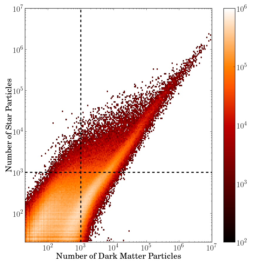
Figure 4: Distribution of the number of dark matter and star particles in subgroups at $z=0.06$, where the colorbar indicates the number density of subhalos.

The reliability of statements about the shapes of matter distributions depends on the number of particles used to trace those distributions. Thus, we made a convergence test to fix the minumum number of particles needed to measure shapes of halos and subhalos reliably. In Fig. 3, we show the histograms of shapes measured using all the dark matter particles in a given subhalo, and compared it with the histograms obtained by using a random subsample of $50$, $300$, $500$ and $1000$ particles in the subhalo. This is done in a mass range where we have enough subhalos with $>1000$ particles. The plots show that using a random subsample of $1000$ particles, we have a good convergence with the shapes determined using all particles. The mean axis ratio, $\langle q\rangle$ is $0.83$ and $\langle s\rangle$ is $0.70$ using all particles. $\langle q\rangle$ varies as $0.77,0.82,0.82,0.83,0.83$ using $50,300,500,1000$ particles respectively. The corresponding values for $\langle s\rangle$ are $0.60,0.68,0.69,0.70,0.70$. Although the mean axis ratios show good convergence with $300$ or $500$ particles, from the plots we can see that the histograms have not converged. Hence, we choose a minimum of $1000$ particles for our analysis. In Figure 4, we show a contour plot of the number of dark matter particles and star particles in subgroups at $z=0.06$. The two different density peaks in the contour plot are due to different dark matter to stellar mass ratios in centrals and satellite subgroups. The right density peak corresponds to central subhalos while the left one is for satellite subgroups, which exhibit stripping of the dark matter subhalo and hence fewer dark matter particles. The lines show a cutoff of $1000$ particles for dark matter and star particles. By choosing this cutoff, we are excluding subhalos of low stellar to halo mass ratio in subhalos around the low mass range $10^{10}-10^{11.5}$$h^{-1}M_{\odot}$. So in this mass range, we are excluding a significant fraction of subhalos with low stellar mass from our analysis. However, in the high mass range, we are able to analyze a fair sample of subhalos.

3 Shapes of dark matter and stellar matter of subgroups

In this section, we show the axis ratio distributions of the shapes of dark matter and stellar matter component of halos and subhalos modeled as ellipsoids as described in Section 2.2. We investigate their dependence on the mass range of subgroups and their evolution with redshift. We also compare the relative axis ratio distributions of dark matter and stellar matter in subhalos.

3.1 3D axis ratio distributuions

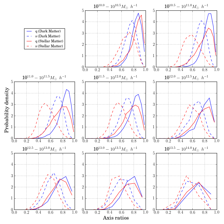
Figure 5: 3d axis ratio distributions of dark matter and stellar matter in subhalos at $z=0.06$, for masses of subhaloes in the range $10^{10.0}-10^{14.0}$$h^{-1}M_{\odot}$.

The distributions of axis ratios, $q~{}(b/a)$ and $s~{}(c/a)$ for dark matter and stellar matter of subgroups at redshift $z=0.06$ for different mass bins are shown in Figure 5. The plot shows that the axis ratios are larger for dark matter when compared to stellar matter, indicating that the dark matter component of a subgroup is more round than the stellar matter. Also, we observe that there is no significant evolution in the distribution of axis ratios in adjacent panels. We henceforth present our results in three mass bins : $10^{10.0}-10^{11.5}$$h^{-1}M_{\odot}$, $10^{11.5}-10^{13.0}$$h^{-1}M_{\odot}$, and $>10^{13.0}$$h^{-1}M_{\odot}$. For convenience, we refer to these mass bins as $M1,M2$ and $M3$ respectively. In the mass bin $M3$, the largest subhalo mass is $1.4\times 10^{14}$$h^{-1}M_{\odot}$ at $z=1.0$, with a host halo mass of $1.6\times 10^{14}$$h^{-1}M_{\odot}$; it grows to $6.0\times 10^{14}$$h^{-1}M_{\odot}$ at $z=0.06$ with a host halo mass of $7.2\times 10^{14}$$h^{-1}M_{\odot}$.

3.2 Redshift evolution and mass dependence of 3D axis ratios

$\begin{array}[]{c@{\hspace{0.5in}}c}\includegraphics[width=231.26378pt,angle={0}]{fig10_0214}\hfil\hskip 36.135pt&\includegraphics[width=231.26378pt,angle={0}]{fig11_0214}\end{array}$

Figure 6: Comparison of axis ratios, $q~{}(b/a)$ (left panel) and $s~{}(c/a)$ (right panel) between dark matter subgroups and groups at $z=0.3$ in different mass bins.

$\begin{array}[]{c@{\hspace{0.5in}}c}\includegraphics[width=231.26378pt,angle={0}]{fig12_0214}\hfil\hskip 36.135pt&\includegraphics[width=231.26378pt,angle={0}]{fig13_0214}\end{array}$

Figure 7: Axis ratios $q~{}(b/a)$ (left panel) and $s~{}(c/a)$ (right panel) for stellar matter of subhalos at $z=0.3$ in mass bins ($M1,M2$ and $M3$) and at $z=1.0,0.06$ for the central mass bin, $M2$.

$\begin{array}[]{c@{\hspace{0.5in}}c}\includegraphics[width=231.26378pt,angle={0}]{q_avg_1113}\hfil\hskip 36.135pt&\includegraphics[width=231.26378pt,angle={0}]{s_avg_1113}\end{array}$

Figure 8: Average axis ratios, $\langle q\rangle$ (left panel) and $\langle s\rangle$ (right panel) for dark matter and stellar component of subhalos as a function of mass, at redshifts $z=1.0,0.3$, and $0.06$.

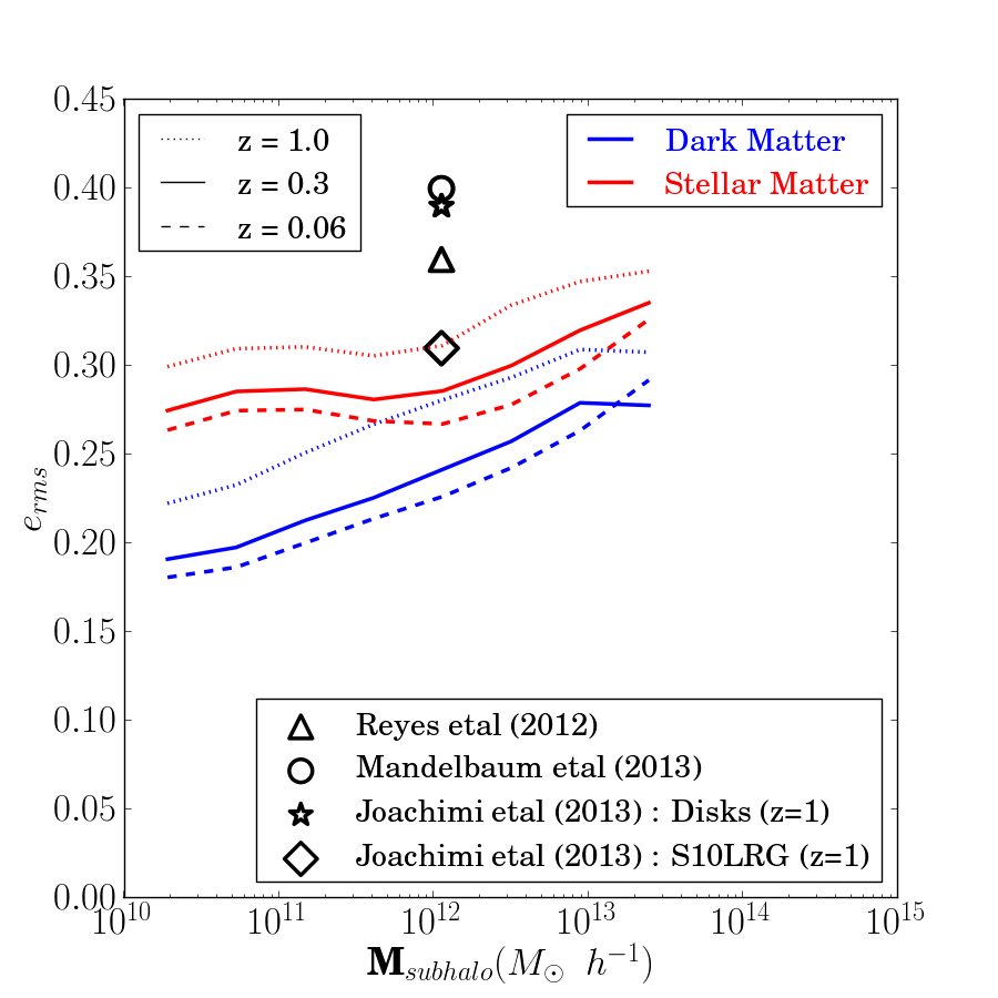
Figure 9: RMS ellipticity per component for projected shapes, $e_{\text{rms}}$, for dark matter and stellar matter at $z=1.0,0.3$, and $0.06$ as a function of cumulative subhalo mass.

In Figure 6, we compare the distribution of axis ratios for groups and subgroups at redshift $z=0.3$ in different mass bins. Here, we consider the dark matter component of groups and subgroups only. From the plot, we can see that for groups, as we go to higher masses, the axis ratios decrease for both groups and subgroups. Comparing the shape distributions between groups and subgroups, we can conclude that the shapes of subgroups are more round when compared to groups in any given mass bin, in agreement with the findings of Kuhlen et al. (2007) using dark matter-only simulation. Even in hydrodynamic simulations, Kazantzidis et al. (2006) found that dark matter subhalos are more round than halos. We can also see that as we go to higher mass bins, the axis ratios of dark matter halos and subhalos decrease in agreement with the findings of Knebe et al. (2008).

To investigate the mass dependence of axis-ratio distributions for the stellar matter component of subgroups, we plot the axis ratios $(q,s)$ at redshifts $z=0.3$ in the mass bins $M1,M2$ and $M3$ in Fig. 7. The plot shows that as we go to higher mass bins, the shapes of subhalos get more flattened. Using the distribution of satellites and Monte Carlo simulations, Wang et al. (2008) reached the same conclusion for dark matter halos. We find that the shapes of stellar matter also follow a similar trend. To understand the redshift evolution of shapes, we also show the shape distributions at $z=1.0$, and $0.06$ for the middle mass bin, $10^{11.5}-10^{13.0}$$h^{-1}M_{\odot}$. The lines show that at lower redshifts, the shapes tend to become rounder. Hopkins et al. (2005), Allgood et al. (2006) and Schneider et al. (2012) used $N$-body simulations and considered the axis ratio distributions as a function of mass and redshift. Their results show that at a given mass, halos are more round at lower redshift, and more massive halos are more flattened which is consistent with our findings. In Fig. 8, we show the average axis ratios, $\langle q\rangle$ and $\langle s\rangle$ as a function of mass at different redshifts $z=1.0,0.3$, and $0.06$ for the dark matter and stellar component. We also provide fitting functions for the average axis ratios of the dark matter and stellar component of subhalos as a function of mass and redshift in Appendix A. The plots for average axis ratios of the dark matter component can be compared against Allgood et al. (2006). Our results agree with theirs qualitatvely in that the average axis ratios, $\langle q\rangle$ and $\langle s\rangle$, increase as we go to lower redshifts and lower masses for the dark matter component. Their curves show a lower average $\langle s\rangle$ which may be because of the different criteria used in the determination of halo shapes, changes in dark matter shapes from the effect of baryons, and different cosmological parameters. Also, they measured average axis ratios for halos, while our results are for subhalos. For the stellar matter, we can see that in general, the average axis ratios decrease with subhalo mass. However, there is an increase in the intermediate mass range around $\sim 10^{11}h^{-1}M_{\odot}$ followed by a decreasing trend once again. We will investigate the dependence of this trend on the type and color of galaxies in a future study to understand the significance of this mass scale.

To compare the axis ratio distributions of projected shapes defined by stellar matter of subhalos with results from observational measurements, we use the statistic, rms ellipticity. The rms ellipticity per single component, $e_{\text{rms}}$, is given by

$$e_{\text{rms}}^{2}=\frac{\sum_{i}{(\frac{1-q_{i}^{\prime 2}}{1+q_{i}^{\prime 2}})}^{2}}{2N},$$ (3)

where $q_{i}^{\prime}=\frac{b_{i}^{\prime}}{a_{i}^{\prime}}$ for the $i^{th}$ subgroup and $N$ is the total number of subgroups considered. In Fig 9, we show the projected rms ellipticity $e_{\text{rms}}$ as a function of cumulative mass of subhalos (by considering all subhalos of mass greater a given mass) for redshifts $z=1.0,0.3$, and $0.06$. Our results can be compared against those from observations in the Sloan Digital Sky Survey (SDSS) given in Reyes et al. (2012). For stellar matter, we obtained $e_{\text{rms}}=0.28$ at $z=0.3$ for $M_{\text{subhalo}}>10^{12}$$h^{-1}M_{\odot}$, which is smaller than the observed value of $0.36$, but reasonably close (and larger than that expected for dark matter component). The catalogue used by Reyes et al. (2012) has been corrected for measurement noise, but it has some selection effects that bias it slightly in the direction of eliminating small round galaxies, thus boosting the RMS ellipticity in the sample of galaxies selected in the data compared to a fair sample. In addition to SDSS, we also made a comparison with observational results obtained using data from COSMOS survey. An $e_{\text{rms}}=0.4$ is obtained using shapes from a galaxy sample in Mandelbaum et al. (2013) with a median redshift of $\sim 0.67$. These galaxies correspond to a mass of $\sim 10^{12}h^{-1}M_{\odot}$ at the median redshift. We made further comparison with measurements on rms ellipticity presented in Joachimi et al. (2013). For a close comparison, we used the results presented for late-type disk dominated galaxies at $z=1$ with the assumption that the sample of galaxies in the simulation is dominated by disks at this redshift. The observational measurements give an rms ellipticity per component of $\sim 0.39$ at $z=1$ which is higher than our values which are in the range of $0.3-0.35$. The lower rms ellipticity may be due to a lower fraction of disk-dominated galaxies in the simulations, or due to the disks not being perfectly realistic. Another comparison is made with a sample of elliptical red galaxies ($S10LRG$) given in Joachimi et al. (2013) where the rms ellipticity per single component is measured to be $~{}\sim 0.31$ at $z=1.0$, in agreement with our result, but no significant redshift evolution of $e_{\text{rms}}$ is detected for this sample. However, the fraction of galaxies in our simulated sample that are red is likely to be a function of redshift. Also, in some of the observations (Reyes et al., 2012; Joachimi et al., 2013), the shape estimator is weighted towards the inner part of the luminosity distribution in a galaxy, while our shape measurements are obtained by considering all the particles of a given type in the subhalo, emphasizing the shape of stellar matter at large radii (similar to the shape estimates in Mandelbaum et al. 2013 from fitting light profiles to galaxy models). Given the known differences between how the measurements in data and simulations were carried out, it is difficult to make a quantitative comparison, however, there are no red flags for a major discrepancy.

4 Misalignments between stellar matter and dark matter shapes of subhalos

In this section, we compare the major axis orientations of the stellar components and dark matter components of subhalos, in 3D and 2D, in order to quantify the degree of misalignment between them. We investigate the dependence of the probability distribution of the misalignments on the mass range of subhalos and redshift. We also discuss the change in misalignments in going from 3D, as defined by the physics, to 2D, which is what we observe for real galaxies. Finally, the misalignments are compared for centrals and satellite subgroups.

4.1 Definition of misalignment angle

For each subgroup, we determined the relative orientation of the major axis of its dark matter subhalo with its stellar component. If $\hat{e}_{ga}$ and $\hat{e}_{da}$ are the major axes of the stellar and dark matter components, respectively, then the misalignment angle is given by

$$\theta_{m}=\arccos(\left|\hat{e}_{da}\cdot\hat{e}_{ga}\right|)$$ (4)

The same definition can be used to determine the misalignment angle in 2D. It is to be noted here that the major axis is not well defined for ellipsoids which are nearly spherical. However, we verified that our results for misalignment angles do not change significantly when we exclude subhalos with $q$ and $s>0.95$ for shapes defined by the dark matter or stellar matter.

4.2 Mass and redshift dependence of misalignments

$\begin{array}[]{c@{\hspace{0.5in}}c}\includegraphics[width=231.26378pt,angle={0}]{fig1_0214_3d}\hfil\hskip 36.135pt&\includegraphics[width=231.26378pt,angle={0}]{fig2_0214_2d}\end{array}$

Figure 10: Histogram of 3D (left panel) and 2D (right panel) misalignments at redshifts $z=1.0,0.3$, and $0.06$ in the mass bins $M1,M2$ and $M3$.

Table 1: Mean 3D misalignments in subgroups at redshifts $z=1.0,0.3$, and $0.06$ in the mass bins $M1,M2$ and $M3$.

Mass ($h^{-1}M_{\odot}$)	Mean 3D misalignment angle
	$z=1.0$	$z=0.3$	$z=0.06$
$M1:10^{10.0}-10^{11.5}$	$31.61^{\circ}$	$33.47^{\circ}$	$34.10^{\circ}$
$M2:10^{11.5}-10^{13.0}$	$20.98^{\circ}$	$25.20^{\circ}$	$27.73^{\circ}$
$M3:~{}>10^{13.0}$	$10.00^{\circ}$	$13.04^{\circ}$	$13.87^{\circ}$

Table 2: Mean 2D misalignments in subgroups at redshifts $z=1.0,0.3$, and $0.06$ in mass bins $M1,M2$ and $M3$

Mass ($h^{-1}M_{\odot}$)	Mean 2D misalignment angle
	$z=1.0$	$z=0.3$	$z=0.06$
$M1:10^{10.0}-10^{11.5}$	$22.61^{\circ}$	$23.78^{\circ}$	$23.88^{\circ}$
$M2:10^{11.5}-10^{13.0}$	$15.51^{\circ}$	$17.89^{\circ}$	$19.41^{\circ}$
$M3:~{}>10^{13.0}$	$8.74^{\circ}$	$10.73^{\circ}$	$11.00^{\circ}$

In Fig. 10, we show the misalignment probability distributions for subgroups at redshifts $z=1.0,0.3$, and $0.06$ in mass bins $M1,M2$ and $M3$. From the plots, we see that in the massive bins, the stellar component is more strongly aligned with its dark matter subhalos. The mean 3D misalignments for each mass bin are listed in Table 1. As we go from lower to higher mass bins, the mean misalignments decrease from $34.10^{\circ}$ to $13.87^{\circ}$. For a given mass bin, the misalignment strength increases towards lower redshifts, as shown in the plot and table; however, the trend with mass is far stronger than the trend with redshift. When comparing 3D and 2D misalignments, we find that the misalignments are more prominent in the 3D situation. This is mainly due to a decrease in misalignment angle by projecting along a particular direction. Also, if we consider random distribution of misalignment angles, it can be inferred geometrically that the probability increases with angle of misalignment in 3D, while the distribution is uniform in 2D. In Appendix B, we give fitting functions for the probability distributions of 3D and 2D misalignment angles in different mass bins at redshifts $z=1.0,0.3,0.06$. These probability distributions of misalignment angles are useful in predicting intrinsic alignment signals and estimating the $C_{1}$ parameter (overall alignment strength) in the linear alignment model (Blazek et al., 2011). Table 2 shows the mean misalignments in 2D. The fitting functions for mean misalignment angles as a function of mass are given in Appendix C. The misalignment distribution for masses $M_{\text{subhalo}}>10^{13}$$h^{-1}M_{\odot}$ shows that the stellar shapes are well aligned with their host dark matter subhalos with a mean misalignment angle of $10.00^{\circ}$ at $z=1$ and $13.87^{\circ}$ at $z=0.06$. In a similar mass range, using $N$-body simulations, Okumura et al. (2009) assumed a gaussian distribution of misalignment angle with zero mean and constrained the width, $\sigma_{\theta}$, to be around $35^{\circ}$ so as to match the observed ellipticity correlation functions for central LRGs. This corresponds to an absolute mean misalignment angle of $\sim 28^{\circ}$. The galaxies used by Okumura et al. (2009) have masses corresponding to our highest mass bin, for which we predict a stronger alignment between dark matter halo and galaxy; however, because of the different methodology used to indirectly derive their misalignment angle compared to our direct prediction from simulations, a detailed comparison is difficult.

5 Shape distributions and misalignments for central vs. satellite galaxies

Here we consider the axis ratio distributions and misalignment probability distributions for central and satellite subgroups in different mass bins, divided in two ways: based on the parent halo mass and based on the individual subhalo mass.

$\begin{array}[]{c@{\hspace{0.5in}}c}\includegraphics[width=231.26378pt,angle={0}]{qstar_halo_0214}\hfil\hskip 36.135pt&\includegraphics[width=231.26378pt,angle={0}]{sstar_halo_0214}\\ \includegraphics[width=231.26378pt,angle={0}]{qstar_sg_0214}\hfil\hskip 36.135pt&\includegraphics[width=231.26378pt,angle={0}]{sstar_sg_0214}\\ \end{array}$

Figure 11: Axis ratio distributions of stellar matter in subgroups for centrals and satellites in mass bins $M1,M2$ and $M3$. Top panel: Results when dividing based on the parent halo mass; bottom panel: when dividing based on the subhalo mass. In both rows, the left and right panels show results for $q$ and $s$, respectively.

$\begin{array}[]{c@{\hspace{0.5in}}c}\includegraphics[width=231.26378pt,angle={0}]{fig7_0214_3d}\hfil\hskip 36.135pt&\includegraphics[width=231.26378pt,angle={0}]{fig78_0214_3d}\end{array}$

Figure 12: Histograms of misalignment angles for central and satellite subgroups in mass bins $M1,M2$ and $M3$. Left: Results when dividing based on the subhalo mass; right: when dividing based on the halo mass.

Table 3: Mean 3D misalignments in central and satellite subgroups at redshifts $z=1.0,0.3$, and $0.06$ in subhalo mass bins $M1,M2$ and $M3$.

	$z=1.0$		$z=0.3$		$z=0.06$
Subhalo Mass ($h^{-1}M_{\odot}$)	Centrals	Satellites	Centrals	Satellites	Centrals	Satellites
$M1:10^{10.0}-10^{11.5}$	$33.42^{\circ}$	$28.21^{\circ}$	$37.07^{\circ}$	$28.22^{\circ}$	$37.83^{\circ}$	$29.00^{\circ}$
$M2:10^{11.5}-10^{13.0}$	$21.30^{\circ}$	$18.03^{\circ}$	$25.85^{\circ}$	$20.43^{\circ}$	$28.68^{\circ}$	$21.54^{\circ}$
$M3:~{}>10^{13.0}$	$9.61^{\circ}$	$17.17^{\circ}$	$13.11^{\circ}$	$11.73^{\circ}$	$14.00^{\circ}$	$12.03^{\circ}$

Table 4: Mean 3D misalignments in central and satellite subgroups at redshifts $z=1.0,0.3$, and $0.06$ in parent halo mass bins $M1,M2$ and $M3$.

	$z=1.0$		$z=0.3$		$z=0.06$
Halo Mass ($h^{-1}M_{\odot}$)	Centrals	Satellites	Centrals	Satellites	Centrals	Satellites
$M1:10^{10.0}-10^{11.5}$	$33.88^{\circ}$	$32.88^{\circ}$	$37.39^{\circ}$	$32.71^{\circ}$	$38.12^{\circ}$	$35.60^{\circ}$
$M2:10^{11.5}-10^{13.0}$	$21.98^{\circ}$	$27.76^{\circ}$	$26.61^{\circ}$	$28.52^{\circ}$	$29.10^{\circ}$	$29.32^{\circ}$
$M3:~{}>10^{13.0}$	$10.33^{\circ}$	$26.10^{\circ}$	$13.47^{\circ}$	$26.48^{\circ}$	$14.76^{\circ}$	$27.36^{\circ}$

In the top panel of Fig. 11, we show normalized histograms of $q$ and $s$ for centrals and satellites binned according to their parent halo mass, for the bins, $M1,M2$ and $M3$. In the bottom panel, we show the same thing, but dividing based on the subgroup masses. The plots show that satellite subgroups are more round than central subgroups. For satellites, we see that the axis ratio distributions show a strong dependence on the subhalo mass and, for $s$, the parent halo mass. These trends go in the opposite direction: satellites tend to have a lower value of $s$ when their parent halo mass is low, or when their subhalo mass is high. If we compare the top and bottom right figures, the minor-to-major axis ratio distributions for centrals exhibit little mass dependence when binning by subhalo mass, but more mass dependence when binning by parent halo mass, suggesting an interesting environment dependence.

In Fig. 12, we show the distributions of the misalignment angles for central and satellite subgroups in different mass bins at redshifts $z=1.0,0.3$, and $0.06$. In the right panel, the binning is based on halo mass, while in the left panel, the binning is according to subhalo mass. We can see that both centrals and satellites exhibit the same qualitative features in the distributions of misalignment angles as the whole sample of subgoups in Fig. 10. Tables 3 and 4 show the mean misalignment angles of centrals and satellites binned binned according to their subhalo and parent halo masses, respectively. Considering mass bins based on individual masses of subhalos, we see that in general, the degree of alignment is larger for satellites than for centrals for all mass bins. However, if we bin based on the mass of the parent halo, then at higher halo masses, central subgroups tend to have larger alignments than the satellite subgroups. This effect may be due to the centrals having higher masses than the satellites, which tends to correlate with having a higher degree of alignment.

6 Conclusions

In this study, we used the MBII cosmological hydrodynamic simulation to study halo and galaxy shapes and alignments, which are relevant for determining the intrinsic alignments of galaxies, an important contaminant for weak lensing measurements with upcoming large sky surveys. While $N$-body simulations have been used in the past to study intrinsic alignments, it is also important to study the effects due to inclusion of the physics of galaxy formation; this includes effects both on the overall shapes (ellipticities) of the galaxies and halos, but also on any misalignment between them. In order to study this particular issue, we measured the shapes of dark matter and stellar component of groups and subgroups.

Previous studies have used $N$-body simulations to study the mass dependence and redshift evolution of the shapes of dark matter halos and subhalos (Lee et al., 2005; Allgood et al., 2006; Kuhlen et al., 2007; Wang et al., 2008; Knebe et al., 2008; Schneider et al., 2012). Our results are qualitatively consistent with several trends identified in previous work. The first such trend that we confirm using SPH simulations is that subhalos are more round than halos (Kazantzidis et al., 2006; Kuhlen et al., 2007). The second trend that we confirm is that the shapes of less massive subhalos are more round than more massive subhalos (Knebe et al., 2008; Wang et al., 2008) and as we go to lower redshifts, the subhalos also tend to become rounder (Hopkins et al., 2005; Allgood et al., 2006; Schneider et al., 2012).

The effect of including baryonic physics on the shapes of dark matter halos was studied previously using hydrodynamic simulations in a box of smaller size and resolution compared to ours (Kazantzidis et al., 2006; Knebe et al., 2010; Bryan et al., 2013). Kazantzidis et al. (2006) found that the axis ratios of dark matter halos increase due to the inclusion of gas cooling, star formation, metal enrichment, thermal supernovae feedback and UV heating. Bryan et al. (2013) found that there is no major effect on shapes under strong feedback, but they observed a significant change in the inner halo shape distributions. Knebe et al. (2010) found that there is no effect on the shapes of dark matter subhaloes, where they included gas dynamics, cooling, star formation and supernovae feedback. Here, we took advantage of the extremely high resolution of MBII to directly study the mass dependence and redshift evolution of the shapes of the stellar component of subhalos in addition to dark matter. However, we did not study the effect of baryonic physics on dark matter shapes by comparison with a reference dark matter only simulation in this work.

We found that the shapes of the dark matter component of subhalos are more round than the stellar component. Similar to dark matter subhalo shapes, the shapes of the stellar component also become more round as we go to lower masses of subhalos and lower redshifts. We are also able to calculate the projected rms ellipticity per single component for stellar matter of subhalos, which can be directly compared with observational results in Reyes et al. (2012). While the observed result is 0.36 at the given mass range, from our simulation, we measured a value of 0.28 at $z=0.3$ for $M>10^{12}$$h^{-1}M_{\odot}$, which is close, particularly given the uncertainties that result from observational selection effects that are not present in the simulations and that drive the RMS ellipticity to larger values, and given the different radial weighting in the two measurements.

By modelling subhalos as ellipsoids in 3D, we are able to calculate the misalignment angle between the orientation of dark matter and stellar component. Previous studies of misalignments in simulations used either low-resolution hydrodynamic simulations, or $N$-body simulations with a scheme to populate halos with galaxies and assign a stochastic misalignment angle and other assumptions (Sharma & Steinmetz, 2005; Heymans et al., 2006; Faltenbacher et al., 2009; Okumura et al., 2009; Hahn et al., 2010; Deason et al., 2011). By direct calculation from our high-resolution simulation data, we found that in massive subhalos, the stellar component is more aligned with that of dark matter, qualitatively similar to results that have been inferred previously through other means. For instance, at $z=0.06$, the mean misalignment angles in mass bins from $10^{10.0}-10^{11.5}$$h^{-1}M_{\odot}$, $10^{11.5}-10^{13.0}$$h^{-1}M_{\odot}$, and $10^{13.0}-10^{15.0}$$h^{-1}M_{\odot}$ are $34.10^{\circ}$, $27.73^{\circ}$, $13.87^{\circ}$, respectively. The amplitude of misalignment increases as we go to lower redshifts. The total mean misalignment angle of $30.05^{\circ}$, $30.86^{\circ}$, $32.71^{\circ}$ at $z=1.0$, $0.3$, $0.06$ respectively shows an increasing trend, though the trend is far weaker than trends with mass at fixed redshift. We also found that the misalignments are larger for 3D shapes when compared to projected shapes. It is to be noted here that we have not split our sample of subhalos according to the type of galaxy. The dependence of our results on galaxy type or color will be investigated in a future study. It is fairly well established that the alignment mechanism for discs and elliptical galaxies is different, so this is a necessary next step to obtain measurements which can be directly compared against observations and used as input for modeling.

Finally, we considered the axis ratios and misalignments in central and satellite subgroups according to their parent halo mass and individual mass of subgroups. We concluded that the shape of stellar component of satellites is more round than that of centrals. We also conclude that the satellite subgroups are more aligned when compared to centrals in similar mass range. Observationally, it is not possible to directly measure the misalignments in centrals and satellites. Misalignment studies for central galaxies were done earlier by Wang et al. (2008); Okumura et al. (2009). Using data and Monte Carlo simulations, Wang et al. (2008) predict a Gaussian distribution of misalignment angle with zero mean and a standard deviation of $23^{\circ}$ for their sample of red and blue centrals. Okumura et al. (2009) used $N$-body simulations and an HOD model for assigning galaxies to halos. The alignment of central LRG’s with host halos is assumed to follow a Gaussian distribution with zero mean. Okumura et al. arrived at a standard deviation of $35^{\circ}$ to match the observed ellipticity correlation. Our predictions of misalignments for central and satellite subgroups are direct measurements that could be done through hydrodynamic simulations which include the physics of star formation.

In conclusion, we found that the axis ratios of the shapes of stellar component of subhalos are smaller when compared to that of dark matter. The shapes of both dark matter and stellar component tend to become more round at low masses and low redshifts. We measured the misalignment between the shapes of dark matter and stellar component and found that the misalignment angles are larger at lower masses and increase slightly towards lower redshifts. We found that the dependence is more on the mass of subhalo than redshift. Finally, we split our subhalos sample into centrals and satellites and found that in similar mass range, the satellites have smaller misalignment angles.

We initiated this study with the goal of predicting intrinsic alignments and constraining their impact on weak gravitational lensing measurements. In this paper, we presented our results on the axis ratios and orientations of both the dark matter and stellar matter of subhalos. Future work will include the dependence of these results on the radial weighting function used to measure the inertia tensor (as in Schneider et al. 2012), galaxy type and the difference between the shape of the stellar mass versus of the luminosity distribution. We will also present our results on the intrinsic alignment two-point correlation functions in a future paper. Finally, future work should include investigation of the impact of changes in the prescription for including baryonic physics in the simulations.

Appendix A Functional forms for dark matter and stellar matter shapes

$\begin{array}[]{c@{\hspace{0.5in}}c}\includegraphics[width=231.26378pt,angle={0}]{fig_avgq_dmfit_n1}\hfil\hskip 36.135pt&\includegraphics[width=231.26378pt,angle={0}]{fig_avgs_dmfit_n1}\end{array}$

Figure 13: Fits for the axis ratios of shape defined by dark matter in subhalos as a function of mass and redshift

$\begin{array}[]{c@{\hspace{0.5in}}c}\includegraphics[width=231.26378pt,angle={0}]{fig_avgq_stfitn6}\hfil\hskip 36.135pt&\includegraphics[width=231.26378pt,angle={0}]{fig_avgs_stfitn6}\end{array}$

Figure 14: Fits for the axis ratios of shape defined by stellar matter in subhalos as a function of mass and redshift

Table 5: Parameters, $\gamma$ and $a_{i}$ for mean axis ratios, $\langle q\rangle$ and $\langle s\rangle$ in mass range, $10^{10.0}-10^{14.0}$$h^{-1}M_{\odot}$

Axis ratio	$\gamma$	$a_{0}$	$a_{1}$	$a_{2}$	$a_{3}$	$a_{4}$	$a_{5}$	$a_{6}$
$q$ (Dark Matter)	-0.12	0.797	-0.049	-	-	-	-	-
$s$ (Dark Matter)	-0.19	0.663	-0.059	-	-	-	-	-
$q$ (Stellar Matter)	-0.14	0.771	-0.004	-0.068	-0.017	-0.061	-0.003	-0.015
$s$ (Stellar Matter)	-0.19	-0.585	0.031	-0.089	-0.034	0.075	-0.001	-0.016

Here, we give the functional forms for the average axis ratios ($q$, $s$) of shapes defined by dark matter and stellar matter in subhalos as a function of mass and redshift. The parameters are given in Table 5. The plots showing fits for mean axis ratios of the shapes of dark matter and stellar matter are given in Figs. 13 and 14 respectively.

The fitting functions for average axis ratios are given by,

$$\langle q,s\rangle=(1+z)^{\gamma}\sum_{i}a_{i}\left[\log(\frac{M}{M_{piv}})\right]^{i}$$ (5)

where, $M_{piv}$ is $10^{12}$$h^{-1}M_{\odot}$.

The fitting functions are linear in $\log(\frac{M}{M_{piv}})$ for shapes of dark matter with $i={0,1}$ and polynomial to $6^{th}$ degree in $\log(\frac{M}{M_{piv}})$ with $i={0,1,2,3,4,5,6}$ for shapes defined by stellar component in subhalos.

Appendix B Functional forms for probability distributions of 3D and 2D misalignment angles

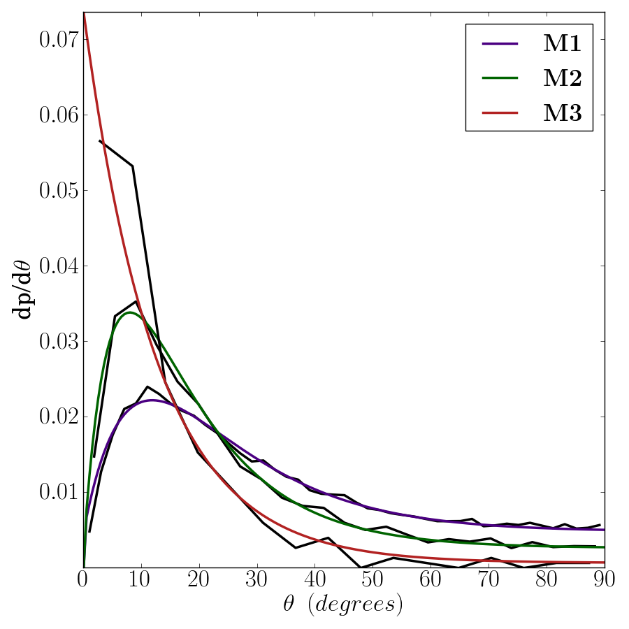
Figure 15: Fits for probability distributions of 3D misalignment angles at $z=0.3$

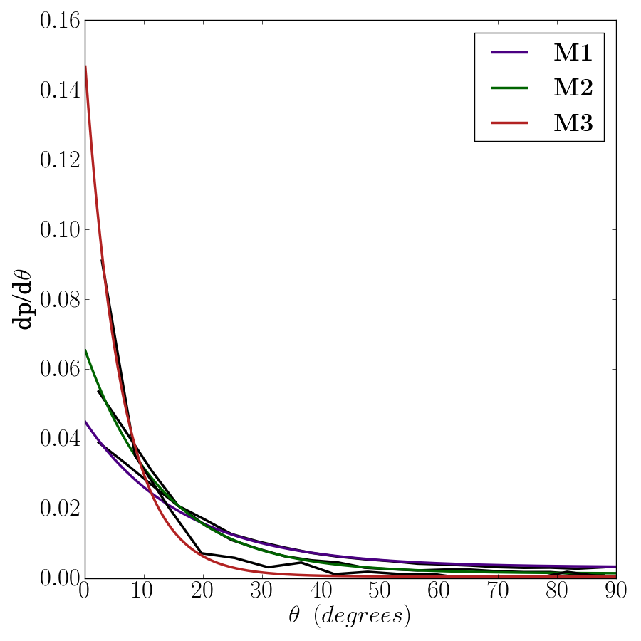
Figure 16: Fits for probability distributions of 2D misalignment angles at $z=0.3$

Table 6: Parameters for probability distributions of 3D misalignment angles at redshifts $z=1.0,0.3$, and $0.06$ for subhalos in the mass bins $M1:10^{10.0}-10^{11.5}h^{-1}M_{\odot},M2:10^{11.5}-10^{13.0}h^{-1}M_{\odot}$ and $M3:~{}>10^{13.0}h^{-1}M_{\odot}$.

	$z=1.0$					$z=0.3$					$z=0.06$
Mass bin	$A_{z}$	$B_{z}$	$C_{z}$	$\gamma_{z}$	$\alpha_{z}$	$A_{z}$	$B_{z}$	$C_{z}$	$\gamma_{z}$	$\alpha_{z}$	$A_{z}$	$B_{z}$	$C_{z}$	$\gamma_{z}$	$\alpha_{z}$
$M1$	$0.211$	$0.079$	$0.004$	$0.023$	$100$	$0.146$	$0.071$	$0.005$	$0.028$	$100$	$0.055$	$0.052$	$0.004$	$0.071$	$100$
$M2$	$0.122$	$0.088$	$0.002$	$0.134$	$100$	$0.091$	$0.074$	$0.003$	$0.121$	$100$	$0.058$	$0.057$	$0.003$	$0.166$	$100$
$M3$	$0.115$	$0.119$	$0.004$	$-$	$-$	$0.073$	$0.079$	$-$	$-$	$-$	$0.064$	$0.070$	$-$	$-$	$-$

Table 7: Parameters for probability distributions of 2D misalignment angles at redshifts $z=1.0,0.3$, and $0.06$ for subhalos in the mass bins $M1:10^{10.0}-10^{11.5}h^{-1}M_{\odot},M2:10^{11.5}-10^{13.0}h^{-1}M_{\odot}$ and $M3:~{}>10^{13.0}h^{-1}M_{\odot}$.

	$z=1.0$			$z=0.3$			$z=0.06$
Mass bin	$A_{z}$	$B_{z}$	$C_{z}$	$A_{z}$	$B_{z}$	$C_{z}$	$A_{z}$	$B_{z}$	$C_{z}$
$M1$	$0.044$	$0.060$	$0.003$	$0.042$	$0.060$	$0.003$	$0.041$	$0.056$	$0.003$
$M2$	$0.077$	$0.089$	$0.001$	$0.064$	$0.075$	$0.002$	$0.056$	$0.069$	$0.002$
$M3$	$0.2$	$0.211$	$0.0$	$0.146$	$0.162$	$0.0$	$0.133$	$0.137$	$0.0$

The probability distributions for 3D misalignment angles in the two lower mass bins $10^{10.0}-10^{11.5}$$h^{-1}M_{\odot}$ and $10^{11.5}-10^{13.0}$$h^{-1}M_{\odot}$ are given by

$$\frac{dp}{d\theta}=A_{z}(1-e^{-\gamma_{z}\theta})e^{-B_{z}\theta}+(1-e^{-\alpha_{z}\theta})C_{z}$$ (6)

In the highest mass bin, $10^{13.0}-10^{15.0}$$h^{-1}M_{\odot}$ the fitting function is,

$$\frac{dp}{d\theta}=A_{z}e^{-B_{z}\theta}$$ (7)

The probability distributions for 2D misalignment angles in different mass bins are given by

$$\frac{dp}{d\theta}=A_{z}e^{-B_{z}\theta}+C_{z}$$ (8)

The fits for the probability distributions in 3D and 2D are shown in Fig. 15 and Fig. 16 respectively and the parameters are given in Tables 6 and 7.

Appendix C Functional forms for mean misalignment angles in 3D and 2D

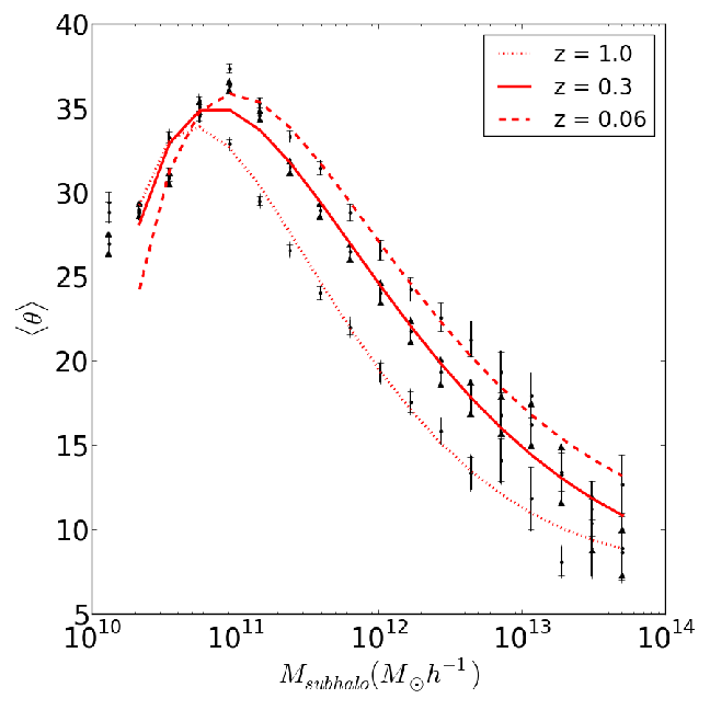
Figure 17: Fits for mean misalignment angles in 3D as a function of mass

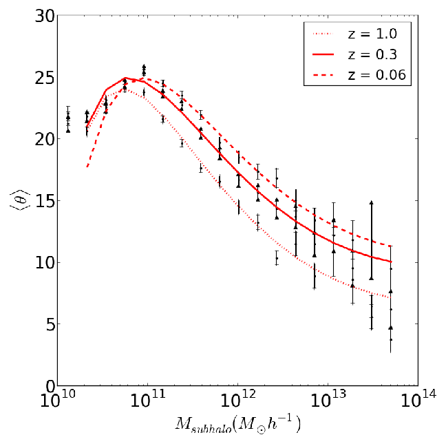
Figure 18: Fits for mean misalignment angles in 2D as a function of mass

Table 8: Parameters for mean misalignment angles in 3D at redshifts $z=1.0,0.3$ and $0.06$ for subhalos in the mass range, $10^{10.0}-10^{14.0}$ $h^{-1}M_{\odot}$.

$z$	$a_{0z}$	$a_{1z}$	$b_{0z}$	$c_{0z}$	$c_{1z}$	$d_{0z}$
$1.0$	$1.19$	$-64.35$	$0.79$	$1.18$	$-11.70$	$10.19$
$0.3$	$0.88$	$-53.72$	$0.97$	$1.16$	$-11.46$	$10.27$
$0.06$	$1.09$	$-28.58$	$0.96$	$1.38$	$-13.74$	$10.84$

Table 9: Parameters for mean misalignment angles in 2D at redshifts $z=1.0,0.3$ and $0.06$ for subhalos in the mass range, $10^{10.0}-10^{14.0}$ $h^{-1}M_{\odot}$.

$z$	$a_{0z}$	$a_{1z}$	$b_{0z}$	$c_{0z}$	$c_{1z}$	$d_{0z}$
$1.0$	$1.44$	$-89.84$	$0.82$	$0.79$	$-7.77$	$9.92$
$0.3$	$1.86$	$-79.50$	$0.89$	$0.89$	$-8.75$	$9.84$
$0.06$	$2.07$	$-43.40$	$0.91$	$0.90$	$-8.99$	$10.47$

The mean misalignment angles in 3D and 2D are given by,

$$\theta(M)=(a_{0z}-a_{1z}e^{-(\frac{\log(M)-d_{0z}}{b_{0z}})})(c_{0z}\log(M)+c_{1z})$$ (9)

The plots showing fits for mean misalignments in 3D and 2D are shown in Fig. 17 and Fig. 18 respectively. The corresponding parameters are given in Tables 8 and 9.

References

- Albrecht et al. (2006) Albrecht A., Bernstein G., Cahn R., Freedman W. L., Hewitt J., Hu W., Huth J., Kamionkowski M., Kolb E. W., Knox L., Mather J. C., Staggs S., Suntzeff N. B., 2006, arXiv, arXiv:astro-ph/0609591
- Allgood et al. (2006) Allgood B., Flores R. A., Primack J. R., Kravtsov A. V., Wechsler R. H., Faltenbacher A., Bullock J. S., 2006, MNRAS, 367, 1781
- Altay et al. (2006) Altay G., Colberg J. M., Croft R. A. C., 2006, MNRAS, 370, 1422
- Bailin et al. (2005) Bailin J., Kawata D., Gibson B. K., Steinmetz M., Navarro J. F., Brook C. B., Gill S. P. D., Ibata R. A., Knebe A., Lewis G. F., Okamoto T., 2005, ApJ, 627, L17
- Benabed & van Waerbeke (2004) Benabed K., van Waerbeke L., 2004, Phys.Rev.D, 70, 123515
- Bernstein & Jain (2004) Bernstein G., Jain B., 2004, ApJ, 600, 17
- Bridle & King (2007) Bridle S., King L., 2007, New Journal of Physics, 9, 444
- Bryan et al. (2013) Bryan S. E., Kay S. T., Duffy A. R., Schaye J., Dalla Vecchia C., Booth C. M., 2013, MNRAS, 429, 3316
- Croft & Metzler (2000) Croft R. A. C., Metzler C. A., 2000, ApJ, 545, 561
- Davis et al. (1985) Davis M., Efstathiou G., Frenk C. S., White S. D. M., 1985, ApJ, 292, 371
- Deason et al. (2011) Deason A. J., McCarthy I. G., Font A. S., Evans N. W., Frenk C. S., Belokurov V., Libeskind N. I., Crain R. A., Theuns T., 2011, MNRAS, 415, 2607
- Di Matteo et al. (2012) Di Matteo T., Khandai N., DeGraf C., Feng Y., Croft R. A. C., Lopez J., Springel V., 2012, ApJ, 745, L29
- Di Matteo et al. (2005) Di Matteo T., Springel V., Hernquist L., 2005, Nature, 433, 604
- Faltenbacher et al. (2002) Faltenbacher A., Gottlöber S., Kerscher M., Müller V., 2002, A&A, 395, 1
- Faltenbacher et al. (2009) Faltenbacher A., Li C., White S. D. M., Jing Y.-P., Shu-DeMao Wang J., 2009, Research in Astronomy and Astrophysics, 9, 41
- Hahn et al. (2010) Hahn O., Teyssier R., Carollo C. M., 2010, MNRAS, 405, 274
- Heavens et al. (2000) Heavens A., Refregier A., Heymans C., 2000, MNRAS, 319, 649
- Heymans et al. (2013) Heymans C., Grocutt E., Heavens A., Kilbinger M., Kitching T. D., Simpson F., Benjamin J., Erben T., Hildebrandt H., Hoekstra H., Mellier Y., Miller L., Van Waerbeke L., Brown M. L., Coupon J., Fu L., Harnois-Déraps J., Hudson M. J., Kuijken K., Rowe B., Schrabback T., Semboloni E., Vafaei S., Velander M., 2013, MNRAS, 432, 2433
- Heymans et al. (2006) Heymans C., White M., Heavens A., Vale C., van Waerbeke L., 2006, MNRAS, 371, 750
- Hirata & Seljak (2004) Hirata C. M., Seljak U., 2004, Phys.Rev.D, 70, 063526
- Hopkins et al. (2005) Hopkins P. F., Bahcall N. A., Bode P., 2005, ApJ, 618, 1
- Hu (2002) Hu W., 2002, Phys.Rev.D, 65, 023003
- Huterer (2010) Huterer D., 2010, General Relativity and Gravitation, 42, 2177
- Ishak et al. (2004) Ishak M., Hirata C. M., McDonald P., Seljak U., 2004, Phys.Rev.D, 69, 083514
- Jing (2002) Jing Y. P., 2002, MNRAS, 335, L89
- Joachimi & Bridle (2010) Joachimi B., Bridle S. L., 2010, A&A, 523, A1
- Joachimi et al. (2011) Joachimi B., Mandelbaum R., Abdalla F. B., Bridle S. L., 2011, A&A, 527, A26
- Joachimi & Schneider (2008) Joachimi B., Schneider P., 2008, A&A, 488, 829
- Joachimi & Schneider (2009) Joachimi B., Schneider P., 2009, A&A, 507, 105
- Joachimi et al. (2013) Joachimi B., Semboloni E., Hilbert S., Bett P. E., Hartlap J., Hoekstra H., Schneider P., 2013, MNRAS, 436, 819
- Katz et al. (1996) Katz N., Weinberg D. H., Hernquist L., 1996, ApJS, 105, 19
- Kazantzidis et al. (2006) Kazantzidis S., Zentner A. R., Nagai D., 2006, in Mamon G. A., Combes F., Deffayet C., Fort B., eds, EAS Publications Series Vol. 20 of EAS Publications Series, The Effect of Baryons on Halo Shapes. pp 65–68
- Khandai et al. (2014) Khandai N., Di Matteo T., Croft R., Wilkins S. M., Feng Y., Tucker E., DeGraf C., Liu M.-S., 2014, arXiv, arXiv:1402.0888
- Knebe et al. (2011) Knebe A., Knollmann S. R., Muldrew S. I., Pearce F. R., Aragon-Calvo M. A., Ascasibar Y., Behroozi P. S., Ceverino D., Colombi S., Diemand J., Dolag K., Falck B. L., Fasel P., Gardner J., Gottlöber S., Hsu C.-H., Iannuzzi F., Klypin A., Lukić Z., Maciejewski M., McBride C., Neyrinck M. C., Planelles S., Potter D., Quilis V., Rasera Y., Read J. I., Ricker P. M., Roy F., Springel V., Stadel J., Stinson G., Sutter P. M., Turchaninov V., Tweed D., Yepes G., Zemp M., 2011, MNRAS, 415, 2293
- Knebe et al. (2010) Knebe A., Libeskind N. I., Knollmann S. R., Yepes G., Gottlöber S., Hoffman Y., 2010, MNRAS, 405, 1119
- Knebe et al. (2008) Knebe A., Yahagi H., Kase H., Lewis G., Gibson B. K., 2008, MNRAS, 388, L34
- Komatsu et al. (2011) Komatsu E., Smith K. M., Dunkley J., Bennett C. L., Gold B., Hinshaw G., Jarosik N., Larson D., Nolta M. R., Page L., Spergel D. N., Halpern M., Hill R. S., Kogut A., Limon M., Meyer S. S., Odegard N., Tucker G. S., Weiland J. L., Wollack E., Wright E. L., 2011, ApJS, 192, 18
- Kuhlen et al. (2007) Kuhlen M., Diemand J., Madau P., 2007, ApJ, 671, 1135
- Lee et al. (2005) Lee J., Jing Y. P., Suto Y., 2005, ApJ, 632, 706
- Mandelbaum et al. (2011) Mandelbaum R., Blake C., Bridle S., Abdalla F. B., Brough S., Colless M., Couch W., Croom S., Davis T., Drinkwater M. J., Forster K., Glazebrook K., Jelliffe B., Jurek R. J., Li I.-H., Madore B., Martin C., Pimbblet K., Poole G. B., Pracy M., Sharp R., Wisnioski E., Woods D., Wyder T., 2011, MNRAS, 410, 844
- Okumura et al. (2009) Okumura T., Jing Y. P., Li C., 2009, ApJ, 694, 214
- Reyes et al. (2012) Reyes R., Mandelbaum R., Gunn J. E., Nakajima R., Seljak U., Hirata C. M., 2012, MNRAS, 425, 2610
- Schneider & Bridle (2010) Schneider M. D., Bridle S., 2010, MNRAS, 402, 2127
- Schneider et al. (2012) Schneider M. D., Frenk C. S., Cole S., 2012, JCAP, 5, 30
- Sharma & Steinmetz (2005) Sharma S., Steinmetz M., 2005, ApJ, 628, 21
- Springel et al. (2005a) Springel V., Di Matteo T., Hernquist L., 2005a, MNRAS, 361, 776
- Springel et al. (2005b) Springel V., Di Matteo T., Hernquist L., 2005b, MNRAS, 361, 776
- Springel & Hernquist (2003a) Springel V., Hernquist L., 2003a, MNRAS, 339, 289
- Springel & Hernquist (2003b) Springel V., Hernquist L., 2003b, MNRAS, 339, 289
- Springel et al. (2001) Springel V., White S. D. M., Tormen G., Kauffmann G., 2001, MNRAS, 328, 726
- Takada & White (2004) Takada M., White M., 2004, ApJ, 601, L1
- Tinker et al. (2008) Tinker J., Kravtsov A. V., Klypin A., Abazajian K., Warren M., Yepes G., Gottlöber S., Holz D. E., 2008, ApJ, 688, 709
- van den Bosch et al. (2003) van den Bosch F. C., Abel T., Hernquist L., 2003, MNRAS, 346, 177
- Wang et al. (2008) Wang Y., Yang X., Mo H. J., Li C., van den Bosch F. C., Fan Z., Chen X., 2008, MNRAS, 385, 1511
- Weinberg et al. (2013) Weinberg D. H., Mortonson M. J., Eisenstein D. J., Hirata C., Riess A. G., Rozo E., 2013, Phys.Rep., 530, 87
- Blazek et al. (2012) Blazek J., Mandelbaum R., Seljak U., Nakajima R., 2012, JCAP, 5, 41
- Blazek et al. (2011) Blazek J., McQuinn M., Seljak U., 2011, JCAP, 5, 10
- Dubois et al. (2014) Dubois Y., Pichon C., Welker C., Le Borgne D., Devriendt J., Laigle C., Codis S., Pogosyan D., Arnouts S., Benabed K., Bertin E., Blaizot J., Bouchet F., Cardoso J.-F., Colombi S., de Lapparent V., Desjacques V., Gavazzi R., Kassin S., Kimm T., McCracken H., Milliard B., Peirani S., Prunet S., Rouberol S., Silk J., Slyz A., Sousbie T., Teyssier R., Tresse L., Treyer M., Vibert D., Volonteri M., 2014, arXiv, arXiv:1402.1165
- Joachimi et al. (2013) Joachimi B., Semboloni E., Bett P. E., Hartlap J., Hilbert S., Hoekstra H., Schneider P., Schrabback T., 2013, MNRAS, 431, 477
- Mandelbaum et al. (2013) Mandelbaum R., Rowe B., Bosch J., Chang C., Courbin F., Gill M., Jarvis M., Kannawadi A., Kacprzak T., Lackner C., Leauthaud A., Miyatake H., Nakajima R., Rhodes J., Simet M., Zuntz J., Armstrong B., Bridle S., Coupon J., Dietrich J. P., Gentile M., Heymans C., Jurling A. S., Kent S. M., Kirkby D., Margala D., Massey R., Melchior P., Peterson J., Roodman A., Schrabback T., 2013, arXiv, arXiv:1308.4982