Theoretical seismology in 3D :
nonlinear simulations of internal gravity waves in solar-like stars

Abstract

Context. Internal gravity waves (hereafter IGWs) are studied for their impact on the angular momentum transport in stellar radiation zones and the information they provide about the structure and dynamics of deep stellar interiors. We present the first 3D nonlinear numerical simulations of IGWs excitation and propagation in a solar-like star.

Aims. The aim is to study the behavior of waves in a realistic 3D nonlinear time-dependent model of the Sun and to characterize their properties.

Methods. We compare our results with theoretical and 1D predictions. It allows us to point out the complementarity between theory and simulation and to highlight the convenience, but also the limits, of the asymptotic and linear theories.

Results. We show that a rich spectrum of IGWs is excited by the convection, representing about 0.4% of the total solar luminosity. We study the spatial and temporal properties of this spectrum, the effect of thermal damping, and nonlinear interactions between waves. We give quantitative results for the modes’ frequencies, evolution with time and rotational splitting, and we discuss the amplitude of IGWs considering different regimes of parameters.

Conclusions. This work points out the importance of high-performance simulation for its complementarity with observation and theory. It opens a large field of investigation concerning IGWs propagating nonlinearly in 3D spherical structures. The extension of this work to other types of stars, with different masses, structures, and rotation rates will lead to a deeper and more accurate comprehension of IGWs in stars.

1 Introduction

IGWs are perturbations propagating in stably stratified regions under the influence of gravity. Planetary atmospheres and stellar radiation zones are therefore ideal places to find them. For example, they can be observed in striated cloud structures in Earth’s atmosphere where they are known to produce large-scale motions such as the quasi-biennial oscillation (QBO) in the lower stratosphere (Plumb & McEwan, 1978; Dunkerton, 1997; Baldwin et al., 2001; Giorgetta et al., 2002). In stars, IGWs propagate in the radiative cores of low-mass stars and the external envelopes of intermediate-mass and massive stars (e.g., Aerts et al., 2010). High-frequency gravity modes have been observed in solar-like stars (e.g., Christensen-Dalsgaard et al., 1995) and more massive stars. IGWs are known for their ability to mix chemical species and to transport angular momentum, affecting the evolution of stars. They can be excited by several processes, depending on the type of stars being considered. In single stars, three excitation processes have been invoked. First, the $\kappa$-mechanism is due to opacity bumps in ionization regions (e.g., Unno et al., 1989; Gastine & Dintrans, 2010). Next, the $\epsilon$-mechanism occurring in massive evolved stars is a modulation of the nuclear reaction rate in the core (e.g., Moravveji et al., 2012). Finally, for solar-type stars, IGWs are mainly excited by stochastic motions such as the pummeling of convective plumes at the interface with adjacent radiative zones (e.g., Hurlburt et al., 1986; Goldreich & Kumar, 1990; Browning et al., 2004; Rogers & Glatzmaier, 2005b; Belkacem et al., 2009; Brun et al., 2011; Shiode et al., 2013; Lecoanet & Quataert, 2013).

The propagation of IGWs in stellar radiative zones can affect their evolution on secular timescales. They have been subject to intense theoretical studies, invoking them to explain several physical mechanisms. With the large-scale meridional circulation (Zahn, 1992; Mathis & Zahn, 2004), the different hydrodynamical shear and baroclinic instabilities (Zahn, 1983), and the fossil magnetic field (Gough & McIntyre, 1998; Brun & Zahn, 2006; Garaud & Garaud, 2008; Duez & Mathis, 2010; Strugarek et al., 2011b), IGWs constitute the fourth main process responsible for the angular momentum redistribution in radiative interiors. Indeed, when they propagate, IGWs are able to transport and deposit a net amount of angular momentum by radiative damping (Press, 1981; Schatzman, 1993; Zahn et al., 1997) and corotation resonances (Booker & Bretherton, 1967; Alvan et al., 2013). Their action induces important changes in the internal rotation profiles of stars during their evolution (Talon & Charbonnel, 2008; Charbonnel et al., 2013; Mathis et al., 2013). In the particular case of the Sun, IGWs are serious candidates to explain the solid body rotation of its radiative interior down to 0.2$R_{\odot}$ (Kumar et al., 1999; Charbonnel & Talon, 2005). They may also provide the extra mixing required to answer the Li depletion question in F stars (Garcia Lopez & Spruit, 1991) and in the Sun (Montalban, J., 1994).

By interfering constructively, IGWs form standing modes also known as gravity (g) modes. Indeed, gravity waves’ frequencies must be inferior to the Brunt-Väisälä (BV) frequency deduced from the characteristics of the star (gravity, density, and pressure profiles). For this reason, IGWs can propagate only in a limited cavity and are susceptible to entering resonance, according to the geometry of this cavity. Such modes have became the object of study of astero- and helioseismology (Aerts et al., 2010; Christensen-Dalsgaard, 1997), together with acoustic (p) modes. Detecting and characterizing g-modes is of great interest for obtaining informations about the inner structure of different types of stars.

For white dwarfs, Landolt (1968) was the first to observe a rapid timescale oscillation in the single white dwarf now known as HL Tau 76. Four years later, Warner & Robinson (1972) and Chanmugam (1972) were able to identify these oscillations with nonradial gravity mode pulsations. Today, an abundance of reports of high-frequency variability in white dwarf stars have been found and used to understand the motions and internal composition of these stars (Vauclair, 2005; Winget & Kepler, 2008). In the case of subdwarf B (sdB) stars, Green et al. (2003) observed a new class of sdB pulsators with periods of about an hour corresponding to gravity modes. And other reports have been made about detections of gravity modes in the upper main-sequence (for example, in slowly pulsating B (SPB) and Be stars) (Waelkens, 1991; De Cat et al., 2011; Neiner et al., 2012). In the past few years, the importance of g-modes have been underlined thanks to the CoRoT and Kepler missions. In particular, the detection of mixed-modes that have the character of g-modes in the core region and of p-modes in the envelope has led to numerous results in red giant seismology (see Mosser et al., 2013, for a complete review). For instance, Bedding et al. (2011) have used them as a way to distinguish between hydrogen- and helium-burning red giants, and they also provide good results for the deduction of the core rotation from the measurement of their rotational splitting (Beck et al., 2012; Mosser et al., 2013; Deheuvels et al., 2012).

However, g-modes remain hardly detectable in the Sun and solar-like stars (Kumar & Quataert, 1995; Turck-Chièze et al., 2004; Appourchaux et al., 2010). Indeed, these stars possess outer convective envelopes where IGWs are evanescent. They thus have a low amplitude when they reach the photosphere level where one could have a chance to detect the oscillations. In past years, intense research have been invested in the quest for the detection of g-modes in the Sun. Both theoretical and numerical works have been undertaken to estimate the solar g-modes’ frequencies (Berthomieu & Provost, 1991) and surface amplitudes (Gough, 1986; Berthomieu & Provost, 1990; Andreassen et al., 1992; Kumar & Quataert, 1995; Andersen, 1996; Belkacem et al., 2009), concluding that most powerfull modes should have amplitudes of about $10^{-3}$ to $10^{-1}$ cm/s (Appourchaux et al., 2010). Detection of g-modes at the surface of the Sun was one of the goals of the SOHO mission (Domingo et al., 1995). Today, asymptotic signatures of gravity modes have been found (Garcia et al., 2007) and used to constrain the rotation of the core (Mathur et al., 2008), but the detection of individual g-modes at the surface of the Sun seems to elude the community.

In parallel with observational and theoretical works, numerical simulations can help for understanding IGWs’ properties and behavior in solar-like stars. In the Sun, the main mechanism for exciting IGWs is convective overshoot. Thus, a series of studies have been performed to determine the extension of convective penetration zone and the resulting excitation of IGWs in 2D (Massaguer et al., 1984; Hurlburt et al., 1986, 1994; Rogers & Glatzmaier, 2005b; Rogers et al., 2006) , and in 3D (Saikia et al., 2000; Brun et al., 2011). Some authors also compared the spectrum of IGWs excited by convection and the energy flux carried by the waves with simpler parametric models of wave generation (Andersen, 1994, 1996; Kiraga et al., 2003, 2005; Dintrans et al., 2005). Finally, the transport of angular momentum by waves has been studied with 1D stellar evolution codes (Talon & Charbonnel, 2005) but also in 2D (Rogers & Glatzmaier, 2006). Here, the use of a realistic stratification in radiation zones is of great importance. Indeed, g-modes are very sensitive to the form of the cavity defined by the BV frequency, particularly for the central region, under 0.2$R_{\odot}$ (Brun et al., 1998; Alvan et al., 2012). For instance, a slight modification of the nuclear reaction rates in the model taken for calculating the BV frequency can induce a frequency shift up to $2\mu$Hz in the range 50-300$\mu$Hz where solar g-modes are expected to be found. Moreover, as shown by Rogers & Glatzmaier (2005a) and Rogers et al. (2008), the effects of wave-wave and wave-mean-flow nonlinear interactions have to be taken into account, which puts nonlinear codes in the foreground.

In the present work, we show results of 3D spherical nonlinear simulations of a full sphere solar-like star. The computational domain extends from 0 to 0.97$R_{\odot}$ by taking the full radiative cavity into account. IGWs are naturally excited by penetrative convection at the interface with the inner radiative zone and can propagate and give birth to standing modes in the cavity. The paper is organized in four sections. After introducing the equations and notations that define the numerical models, we show in Sect. 3 that a rich spectrum of IGWs is excited by convective penetration. In Sect. 4, we examine the properties of this spectrum precisely, highlighting its richness where both modes and propagating waves are present. We give quantitative results about the group velocity of such waves, we measure their period spacing, their lifetime, and the splitting induced by the rotation. Lastly, Sect. 5 presents our results concerning the waves’ amplitude and the effect of the radiative damping affecting their propagation. In particular, we discuss the effect of the diffusivities on the amplitude of waves and the nonlinear wave-wave interactions.

2 Numerical model

2.1 Equations

Following Brun et al. (2011), we use the hydrodynamic ASH code (Clune et al., 1999; Brun et al., 2004) to solve the full set of 3D anelastic equations in a rotating star, treating radiative and convective regions and their interface simultaneously. These equations are fully nonlinear in velocity, and thermodynamic variables are linearized with respect to a spherically symmetric and evolving mean state. We note $\bar{\rho}$, $\bar{{P}}$, $\bar{{T}}$, and $\bar{{S}}$ the reference density, pressure, temperature and specific entropy.
Fluctuations about this reference state are denoted by $\rho$, ${P}$, ${T}$, and ${S}$. We assume a linearized equation of state

$$\frac{\rho}{\bar{\rho}}=\frac{{P}}{\bar{{P}}}-\frac{{T}}{\bar{{T}}}=\frac{{P}}{\gamma\bar{{P}}}-\frac{{S}}{c_{p}}\hbox{,}$$ (1)

and the zeroth-order ideal gas law

$$\bar{{P}}=\mathcal{R}\bar{\rho}\bar{{T}}\hbox{,}$$ (2)

where $\gamma$ is the adiabatic exponent, $c_{p}$ the specific heat per unit mass at constant pressure, and $\mathcal{R}$ the gas constant. The continuity equation in the anelastic approximation is

$$\@vec{\nabla}.\left(\bar{\rho}\@vec{{\mathrm{v}}}\right)=0\hbox{,}$$ (3)

where ${\mathrm{v}}=\left({\mathrm{v}}_{r},{\mathrm{v}}_{\theta},{\mathrm{v}}_{\varphi}\right)$ is the local velocity expressed in spherical coordinates $\left(r,\theta,\varphi\right)$ in the frame rotating at constant angular velocity $\@vec{\Omega}_{0}=\@vec{\Omega}_{0}\@vec{e_{z}}$. The usual momentum equation is

$$\bar{\rho}\left(\frac{\partial\@vec{{\mathrm{v}}}}{\partial t}+\left(\@vec{{\mathrm{v}}}.\@vec{\nabla}\right)\@vec{{\mathrm{v}}}\right)=-\@vec{\nabla}{P}+\rho\@vec{{g}}-2\bar{\rho}\@vec{\Omega}_{0}\times\@vec{{\mathrm{v}}}-\@vec{\nabla}.\@vec{\mathcal{D}}-\left[\@vec{\nabla}\bar{{P}}-\bar{\rho}\@vec{{g}}\right]\hbox{,}$$ (4)

where $\@vec{{g}}$ is the gravitational acceleration, and $\mathcal{D}$ the viscous stress tensor defined by

$$\mathcal{D}_{ij}=-2\bar{\rho}\nu\left(e_{ij}-1/3\left(\@vec{\nabla}.\@vec{{\mathrm{v}}}\right)\delta_{ij}\right)\hbox{,}$$ (5)

with $e_{ij}=1/2\left(\partial_{j}{\mathrm{v}}_{i}+\partial_{i}{\mathrm{v}}_{j}\right)$ the strain rate tensor and $\delta_{ij}$ the Kronecker symbol. The bracketed term on the righthand side of Eq. (4) is initially zero because the system begins in hydrostatic balance. Then, as the simulation evolves, the reference state is driven away from this balance by turbulent pressure.

Brown et al. (2012) have shown that depending on the used anelastic formulation, the quality of the conservation of energy in stably-stratified atmospheres varies. In particular, when modeling highly stratified radiative interiors, the energy in waves may be overestimated. As a consequence, instead of the classical formulation, Brown et al. (2012) advocate implementing the Lantz-Braginsky-Roberts (LBR) (e.g., Lantz, 1992; Braginsky & Roberts, 1995) equations that treat the reduced pressure $\widetilde{\omega}=P/\bar{\rho}$ instead of the fluctuating pressure $P$. In ASH, the new momentum equation is thus

$$\bar{\rho}\left(\frac{\partial\@vec{{\mathrm{v}}}}{\partial t}+\left(\@vec{{\mathrm{v}}}.\@vec{\nabla}\right)\@vec{{\mathrm{v}}}\right)=-\bar{\rho}\@vec{\nabla}\widetilde{\omega}-\bar{\rho}\frac{S}{c_{p}}\@vec{g}-2\bar{\rho}\@vec{\Omega}_{0}\times\@vec{{\mathrm{v}}}-\@vec{\nabla}.\@vec{\mathcal{D}}\hbox{,}$$ (6)

where only the contribution of entropy fluctuations remains in the buoyancy term, the contribution due to pressure perturbations being included in the reduced pressure gradient.
It is important to note that, in this formulation, we neglect the extra buoyancy term relative to the nonadiabatic reference state in the radiative region. This assumption is based on energy conservation arguments developed in Brown et al. (2012). Finally, the equation of conservation of energy remains unchanged

$$\bar{\rho}\bar{{T}}\frac{\partial{S}}{\partial t}+\bar{\rho}\bar{{T}}\@vec{{\mathrm{v}}}.\@vec{\nabla}\left({S}+\bar{{S}}\right) = \bar{\rho}\epsilon+\@vec{\nabla}.\left[\kappa_{r}\bar{\rho}c_{p}\@vec{\nabla}\left({T}+\bar{{T}}\right)\right.$$ (7)

$$\left.+\kappa\bar{\rho}\bar{{T}}\@vec{\nabla}{S}+\kappa_{0}\bar{\rho}\bar{{T}}\@vec{\nabla}\bar{{S}}\right] + 2\bar{\rho}\nu\left[e_{ij}e_{ij}-1/3\left(\@vec{\nabla}.\@vec{{\mathrm{v}}}\right)^{2}\right]\hbox{,}$$

where $\kappa_{r}$ is the radiative diffusivity based on a 1D solar structure model. As perturbations and motions can occur on smaller scales than our grid resolution, the effective eddy diffusivities $\nu$ and $\kappa$ represent momentum and heat transport by subgrid-scale (SGS) motions that are unresolved by the simulation. Their profiles are functions of radius chosen for each model depending on its objectives. The functions chosen in this work are detailed in Sect. 2.4 and represented in Fig. 2.
The diffusivity $\kappa_{0}$ is part of the SGS treatment in the convective zone. It is set such as to have the unresolved eddy flux (entropy flux) carrying the solar flux outward the top of the domain (see left panel of Fig. 1). It drops off exponentially with depth to ensure that it does not play any role in the radiative zone (Miesch et al., 2000). In Eq. (Appendix A: Inner boundary conditions), a volume-heating term $\bar{\rho}\epsilon$ is also included, representing energy generation by nuclear burning. We have assumed a simple representation of the nuclear reaction rate by setting $\epsilon=\epsilon_{0}{T}^{k}$, with $\epsilon_{0}$ a constant determined such that the radially integrated heating term equals the solar luminosity at the base of the convection zone and $k=9$. The exponent $k$ is chosen to obtain a heating source term in agreement with that of a 1D standard model (Brun et al., 2002), considering both contributions of the p-p chains and CNO cycles.

2.2 Boundary conditions and time-step control

In this paper, we have compared various models of the Sun. For all of them, the computational domain extends from $r_{\mathrm{bot}}$ = 0 to $r_{\mathrm{top}}$ = 0.97$R_{\odot}$ where $R_{\odot}=6.96\times 10^{10}$cm is the solar radius. For the problem to be well posed, we thus need to define boundary conditions. At the top of the domain, we have opted for torque-free velocity conditions and constant heat flux (Brun et al., 2011):

1. rigid: $\left.\mathrm{v}_{r}\right\lvert_{r_{\mathrm{top}}}=0$,
   

2. stress-free: $\left.\displaystyle\frac{\partial}{\partial r}\left(\frac{\mathrm{v}_{\theta}}{r}\right)\right\lvert_{r_{\mathrm{top}}}=\left.\displaystyle\frac{\partial}{\partial r}\left(\frac{\mathrm{v}_{\varphi}}{r}\right)\right\lvert_{r_{\mathrm{top}}}=0$,
   

3. constant mean entropy gradient:
   $\displaystyle\frac{\partial\bar{S}}{\partial r}\biggr{\lvert}_{r_{\mathrm{top}}}=-1.5\times 10^{-7}$cm.K^-1.s^-2.

The inner boundary conditions are special because another new feature of the ASH code is that we are now able to extend our computational domain to $r=0$. Indeed, the central singularity requires special attention. Following Bayliss et al. (2007), we have implemented regularity conditions imposing that only $\ell=1$ mode can go through the center and adapted the thermal conditions. In the code, we use the poloidal-toroidal decomposition

$$\bar{\rho}\@vec{\mathrm{v}}=\@vec{\nabla}\times\@vec{\nabla}\times\left(W\@vec{e_{r}}\right)+\@vec{\nabla}\times\left(Z\@vec{e_{r}}\right)\hbox{,}$$ (8)

which ensures that the mass flux remains divergenceless (see Eq. (3)). The conditions in $r=0$ thus translate to

• $Z=0$ for all $\ell$,
  

• $W=0$ and $\displaystyle\frac{\partial W}{\partial r}=0$ for $\ell=1$,
  

• $W=0$ and $\displaystyle\frac{\partial^{2}W}{\partial r^{2}}=0$ for $\ell\neq 1$,
  

• $\bar{S}=0$ for $\ell\neq 0$,
  

• $\displaystyle\frac{\partial\bar{S}}{\partial r}=0$ for $\ell=0$.
  

The detail of the calculation is developed in Appendix A. Since the number of constraints is higher than the number of conditions, we explain our choice and show that another set of boundary conditions gives the same result at 0.1%.

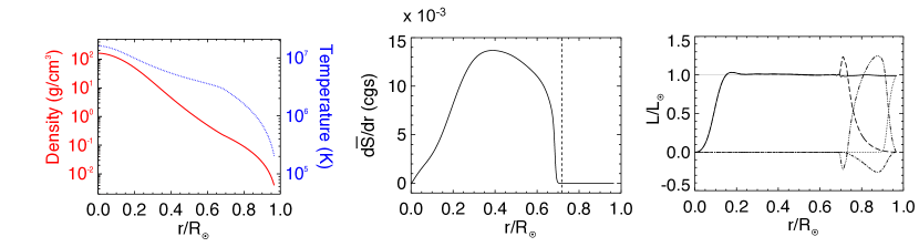
Figure 1: Left: Radial profiles of the reference density $\bar{\rho}$ (red / solid line) and temperature $\bar{T}$ (blue / dotted line) as a function of the normalized radius. Middle: Radial profiles of the entropy gradient. The vertical dotted line marks the radius where $d\bar{S}/dr$ changes sign. It corresponds to the initial limit between convective and radiative zones. Right: Radial energy flux balance converted into luminosity and normalized to the solar luminosity $L_{\odot}$. The values have been averaged over latitude, longitude and time ($\approx$ 30 days). We show the contribution to the energy flux from radiative diffusion (long dashes), enthalpy (three-dot-dashed), kinetic energy (dash-dot), modeled SGS processes (dot), and viscous diffusion (dashes). The solid line is the sum of all these components.

Owing to the convergence of the mesh size as we get closer to $r=0$, the horizontal Courant-Friedrichs-Lewy (CFL) condition

$$\tau^{\displaystyle\mathrm{h}}_{\mathrm{CFL}}=\sqrt{\frac{r^{2}}{\ell_{\mathrm{max}}(\ell_{\mathrm{max}}+1)\mathrm{v}_{\mathrm{h}}^{2}}}\hbox{,}$$ (9)

with $\mathrm{v}_{\mathrm{h}}=\sqrt{\mathrm{v}_{\theta}^{2}+\mathrm{v}_{\varphi}^{2}}$, becomes too extreme if we retain all the $\ell$ values. We thus apply a filter as we get closer to the center that asymptotes to $\ell=1$ since only this component of the flow is allowed to go through. The thermodynamic variables are not affected by this modification. To assess the radial dependence of the filter and rather than imposing a functional shape, we evaluate the horizontal velocity spectrum at each depth and time step and retain scales with $p_{\mathrm{tol}}$ of the peak value, using the usual choice $p_{\mathrm{tol}}=10^{-3}$ . The horizontal CFL condition thus becomes

$$\tau^{\displaystyle\mathrm{h}}_{\mathrm{CFL}}=\sqrt{\frac{r^{2}}{\ell_{\mathrm{eff}}(\ell_{\mathrm{eff}}+1)\mathrm{v}^{2}_{\mathrm{h}}}}\hbox{,}$$ (10)

with $\ell_{\mathrm{eff}}\underset{r\to 0}{\longrightarrow}1$. We tested several values of $p_{\mathrm{tol}}$ and did not noticed significant changes in the wave spectrum. We finally impose a maximum time step

$$\tau_{\mathrm{CFL}}=\mathrm{min}\left(\tau^{\displaystyle\mathrm{r}}_{\mathrm{CFL}},\tau^{\displaystyle\mathrm{h}}_{\mathrm{CFL}}\right)\hbox{,}$$ (11)

with

$$\tau^{\displaystyle\mathrm{r}}_{\mathrm{CFL}}=\frac{\mathrm{min}\left({\Delta r}\right)}{\mathrm{max}(|\mathrm{v}_{r}|)}\hbox{.}$$ (12)

Parameter	ref	therm1	therm2	turb1	turb2
($N_{r}$,$N_{\theta}$,$N_{\varphi}$)	(1581,256,512)	(1581,256,512)	(1581,256,512)	(1581,256,512)	(1581,512,1024)
$\nu_{\mathrm{top}}(\mathrm{cm}^{2}/$s)	$4\times 10^{12}$	$4\times 10^{12}$	$4\times 10^{12}$	$2\times 10^{12}$	$1\times 10^{12}$
$\nu_{\mathrm{exp}}$	$10^{-3}$	$10^{-3}$	$10^{-3}$	$10^{-3}$	$10^{-3}$
$\kappa_{\mathrm{top}}(\mathrm{cm}^{2}$/s)	$3.2\times 10^{13}$	$3.2\times 10^{13}$	$3.2\times 10^{13}$	$1.6\times 10^{13}$	$0.8\times 10^{13}$
$\kappa_{\mathrm{exp}}$	$10^{-4}$	$10^{-3}$	$10^{-2}$	$10^{-4}$	$10^{-4}$
$P\mathrm{r}$ in CZ	0.125	0.125	0.125	0.125	0.125
$P\mathrm{r}$ in RZ	1.25	0.125	0.0125	1.25	1.25
$Re$	169	169	169	338	675

Table 1: $N_{r}$, $N_{\theta}$, and $N_{\varphi}$ are the radial, latitudinal, and longitudinal mesh points. turb2 is the more turbulent model so we doubled its horizontal resolution to ensure that the fluid motions are well resolved. When it is convenient, we distinguish between convection zone (CZ) and radiative zone (RZ). $P\mathrm{r}=\nu/\kappa$ is the Prantdl number, $R\mathrm{e}=VL/\nu$ the Reynolds number where $L=0.97R_{\odot}$ and $V$ is the rms convective velocity.

2.3 Numerical resolution

To initialize the 3D simulation, we specify a reference state derived from a 1D solar structure model (Brun et al., 2002). We impose the entropy gradient $d\mathrm{\bar{S}}/dr$ and the gravitational acceleration $g$ based on the 1D model and then deduce the reference density $\bar{\rho}$ from the equation of hydrostratic equilibrium and the ideal gas law (Eq. (2)) using a Newton-Raphson method. The left and middle panels of Fig. 1 show the reference density, temperature, and entropy gradient. In the middle panel, if $d\bar{S}/dr>0$ then the BV frequency (see following sections) is real and positive and IGWs can propagate in this region. In the convective region, $d\bar{S}/dr<0$, and that translates into IGWs being evanescent. During the simulation, these reference values are updated using the spherically averaged perturbation fields. After having evolved the model over several convective overturning times, we obtain the flux balance represented in the righthand panel of Fig. 1. The different contributions to the energy flux are represented. In the convective envelope, the inward kinetic energy flux due to the asymmetry between up- and downflows is balanced by the outward enthalpy flux that exceeds the solar luminosity and carries the main part of the energy in this zone. We note the penetration of convective motions below the convection zone. The system is expected to adjust to a new equilibrium by modifying the background thermal stratification (e.g., Zahn, 1991) but the relaxation timescale is too long (about $10^{5}$ yr) to be achieved in the simulation. For this reason, we speed up the relaxation process by increasing the radiative diffusivity $\kappa_{r}$ and the associated radiation flux at the base of the convective zone to balance the inward enthalpy flux (Miesch et al., 2000; Brun et al., 2011). In the radiative zone, the main contribution to the total flux is brought by the radiative flux. Finally, the entropy flux represents the flux carried by the unresolved motions and is confined to the upper layers.

For the numerical resolution, the velocity and thermodynamic variables are expanded in spherical harmonics $Y_{\ell,m}(\theta,\varphi)$ for their horizontal structure. For the radial structure we use a finite-difference approach on a non uniform grid, unlike Brun et al. (2011) where the variables were expanded in two Chebyshev polynomials $T_{n}(r)$ in the radial direction. This new feature of the code has been tested by comparing results in simpler setting with the previous version (with Chebyshev decomposition) and with the anelastic benchmark problems of Jones et al. (2011). The agreements are as good, if not better than with the Chebyshev expansion (Featherstone et al. 2013, private communication). Then, following Glatzmaier (1984), we use an explicit Adams-Bashforth time integration scheme for the advection and Coriolis terms, and a semi-implicit Crank-Nicholson treatment for the diffusive and buoyancy terms (Clune et al., 1999).

2.4 Models

All of the models described in this paper are based on the same reference state. We distinguish five models of the Sun where we have chosen different diffusion coefficients. The radial profiles of $\nu$ and $\kappa$ are

$$\nu(r) = \nu_{\mathrm{top}}\left[\nu_{\mathrm{exp}}+f(r)(1-\nu_{\mathrm{exp}})\right]\hbox{,}$$ (13)

$$\kappa(r) = \kappa_{\mathrm{top}}\left[\kappa_{\mathrm{exp}}+f(r)(1-\kappa_{\mathrm{exp}})\right]\hbox{,}$$ (14)

where

$$f(r)=\frac{1}{2}\left[\tanh\left(\frac{r-r_{t}}{\sigma_{t}}\right)+1\right]\hbox{.}$$ (15)

The radius $r_{t}$ = $4.86\times 10^{10}$cm and stiffness $\sigma_{t}=0.04\times 10^{10}$cm are identical for all models. The difference concerns the choice of $\nu_{\mathrm{top}}$, $\nu_{\mathrm{exp}}$, $\kappa_{\mathrm{top}}$, and $\kappa_{\mathrm{exp}}$ referenced in Tab 1.

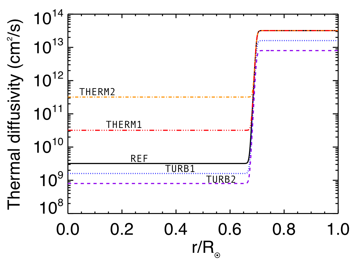
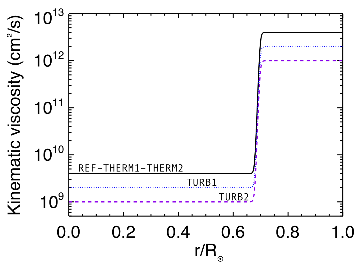
Figure 2: Diffusion coefficients $\nu$ and $\kappa$ (cm²/s) for the five models presented in the article. The corresponding parameters are detailed in Tab 1.

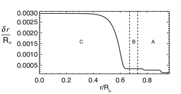
Figure 3: Spacing (in solar radius) between two consecutive radial levels as a function of the normalized radius. Zone A (1012 points, $0.24R_{\odot}$) represents the main part of the convective zone. Zone B (179 points, $0.06R_{\odot}$) corresponds to the interface region where the kinematic viscosity and the thermal diffusivity drop abruptely. And zone C (390 points, $0.67R_{\odot}$) is the radiative zone.

These profiles are chosen to study the thermal and viscous effects of the fluid on the waves. The main model that will be used in the following sections is called ref. Its diffusion coefficients were selected to obtain the clearer possible pattern and spectrum of gravity waves. Indeed, it is known that gravity waves are damped during their propagation by a factor depending on the fluid’s radiative diffusivity (Zahn et al., 1997). Models therm1 and therm2 were computed to study the effect of this damping. They differ from ref only in the radiative zone where their $\kappa$ coefficient is 10 (therm1) and 100 (therm2) times higher (see Fig. 2). On the other hand, we expect a stronger wave’s excitation with a more turbulent convection. For this reason, we discuss two other models called turb1 and turb2 where the Reynolds number $R\mathrm{e}=VL/\nu$ ($V$ and $L$ are characteristic velocity and length scale) is increased by factors 2 and 4 in comparison with ref. An overview of these diffusivities is given in Fig. 2.
In the convective zone, all models have the same Prandtl number $P\mathrm{r}=\nu/\kappa=0.125$. In the radiative zone, however, these values differ (see Tab 1) and have different impacts on the amplitude of the waves observed in the radiative zone. We discuss this point further in Sect. 5.3. The horizontal and radial resolutions of the models are also indicated in Tab 1. In particular, the choice of the radial grid requires attention in order to deal with the strong entropy and diffusivity gradients at the interface between convective and radiative zones. The total number of radial points in the five models is $1581$. We show their distribution in Fig. 3. The number of points in zone C (radiative zone) allows a good compromise between the resolution needed to deal with gravity waves, the stability of the models near the center, and the cost of the total simulation.
Finally, we note that all models rotate at the solar rotation rate, $\Omega_{\odot}=2.6\times 10^{-6}$ rad/s. About 130 turnover times after the beginning of the simulation, we observe a differential rotation in the convective zone as shown in Fig. 4 for model ref. The equator rotates faster than the poles, and we retrieve a conical shape at mid-latitude, as deduced by helioseismology (e.g., Thompson et al., 2003). Since model ref is more turbulent than the one published in Brun et al. (2011), the overall $\Delta\Omega$ contrast is about 130 nHz. The sharp transition to solid body rotation in the radiative zone (i.e., the tachocline). This rotation profile is due to our uniform initial conditions and is maintained during the simulation because the total computed time is shorter than the radiative spreading time (Spiegel & Zahn, 1992). For more details concerning the confinement of the solar tachocline, see Brun & Zahn (2006) and Strugarek et al. (2011a). This bulk rotation have a visible effect on IGWs that is discussed in Sect. 4.3.2.

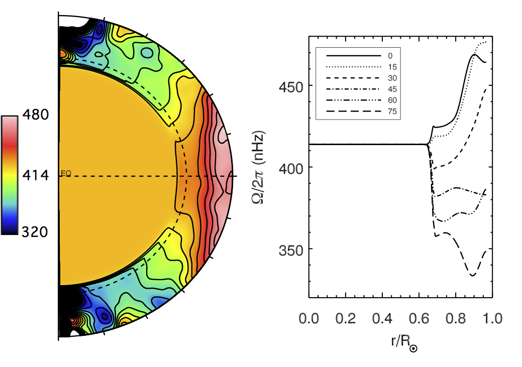
Figure 4: Differential rotation profile of the model ref. Left: Angular velocity $\Omega(r,\theta)=\displaystyle\frac{V_{\varphi}}{r\sin\theta}+\Omega_{0}$ averaged over longitude and time. Dashed lines represent the equator and the interface between convective and radiative zones. Right: Radial cuts of $\Omega$ at selected latitudes. We clearly see the differential rotation affecting the convective zone, the shear layer at the base of the convection zone (tachocline), and the flat rotation profile in the radiative zone.

3 Excitation of gravity waves

Due to the coupling between convective and radiative zones, waves are excited and propagate in the inner radiative zone. Figure 5 shows a 3D view of model ref where we clearly see these waves by removing a quadrant of the sphere. Colors correspond to radial velocity. The convective pattern in the outer zone is visible with blue downward flows and red upward flows. In the radiative zone, spherical patterns correspond to the wavefronts of gravity waves. For the sake of the visualization, the amplitude of $\mathrm{v}_{r}$ has been normalized by its root mean square at each radius, making the waves appear as if their amplitude was about the same as the velocity in the convective zone. In reality, there is a drop of amplitude of six to ten orders of magnitude between both zones, depending on the model, as we will discuss in Fig. 28. In this section, we show how the penetration of convective plumes in the radiative zone excites the rich spectrum of gravity waves that is observed.

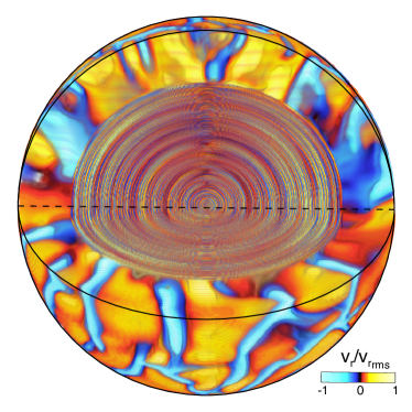
Figure 5: 3D representation of the normalized radial velocity in the full simulated star (model ref). A quadrant of the sphere has been removed to show the wave pattern in the radiative zone.

3.1 Penetrative convection

Several processes have been invoked to explain the excitation of gravity waves in stars. Their relative efficiency differ with the type of star. In the case of the Sun and solar-like stars, the main excitation process is the pummeling of convective plumes at the interface between convective and radiative zones. Indeed, the convection does not stop abruptly at the interface with the radiative zone. When convective plumes reach this boundary, their inertia makes them penetrate the radiative region. Then they are forced to slow down by buoyancy, and the loss of kinetic energy is converted into gravity waves, as discussed in detail in Brun et al. (2011).

In Fig. 6 we represent the radial velocity and the temperature fluctuations realized in the model ref at the top of the computational domain (r=0.97$R_{\odot}$). Convective motions are apparent as a network of narrow cool downflow lanes (dark/blue) surrounding broader warmer upflows (red). This pattern varies with time, convective cells continuously emerging and merging with one another or splitting into several distinct structures. If we move deeper into the convection zone (Brun et al., 2011), isolated plumes appear, corresponding to the strongest downflows that managed to go through the entire convective envelope.

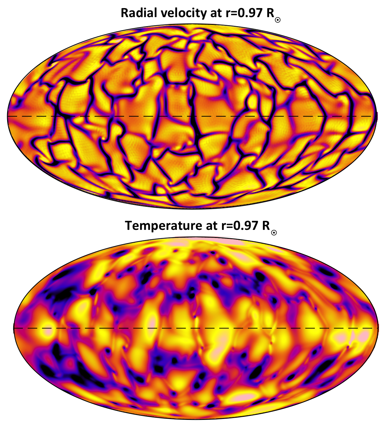
Figure 6: Mollweide projection of the radial velocity and temperature fluctuations at r=0.97$R_{\odot}$ for the model ref. The horizontal dashed line corresponds to the equator. Dark tones denotes negative (inward) velocities and temperature fluctuations.

As explained in Sect. 2.4, we have computed several models with different diffusivity coefficients. In particular, the convective turbulence increases from model ref to turb2 (their Reynolds numbers are given in Tab 1). We see later that IGWs are excited in turb2 with a higher amplitude than in ref. Indeed, the radial enthalpy profile at the interface with radiative zone is different in these two models. We represent a radial cut of an azimuthal and temporal average of the radial enthalpy flux for both models in Fig. 7. The negative peaks of enthalpy flux at the base of the convection zone characterize the buoyant braking of convective plumes. We clearly see that this peak is thinner and more pronounced for turb2. Moreover, the measure of the rms velocity of the fluid just above the radiative zone (the limit is defined by the change of sign of the entropy gradient $d\bar{S}/dr$) shows that the plumes in turb2 are quicker than in ref.

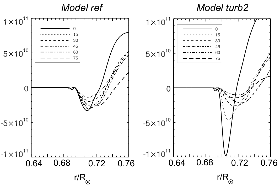
Figure 7: Radial cuts of azimuthal and temporal averages of the radial enthalpy flux in models ref and turb2 at specified latitudes zooming into the overshoot region.

3.2 Excitation of gravity waves: St Andrew’s cross

Thanks to a zoom in the region of penetration shown in Fig. 9, we retrieve a classical result of fluid mechanics concerning the excitation of IGWs by a localized disturbance in a stably stratified fluid (Lighthill, 1978; Voisin, 1991). When we neglect the rotation, the linearized dispersion relation for gravity waves is

$$\omega=\frac{Nk_{h}}{\sqrt{k_{r}^{2}+k_{h}^{2}}}\hbox{,}$$ (16)

where $\omega$ is the frequency of the wave (in Hz), and $\@vec{k}=k_{r}\@vec{e}_{r}+\@vec{k}_{h}$ the wavevector decomposed into its radial and horizontal parts. The Brunt-Väisälä frequency (given in Hz)

$$N=\frac{1}{2\pi}\sqrt{-\bar{g}\left(\frac{1}{\bar{\rho}}\frac{\partial\bar{\rho}}{\partial r}-\frac{1}{\Gamma_{1}\bar{P}}\frac{\partial\bar{P}}{\partial r}\right)}$$ (17)

describes the stratification in density in the radiative zone.

Figure 8: Radial profile of the Brunt-Väisälä frequency $N$ (common to all models).

The profile of $N$ is shown in Fig. 8. It is real and positive in the radiative zone (that corresponds to the positive entropy gradient shown in Fig. 1) and becomes purely imaginary for $r>0.717R_{\odot}$, where the entropy gradient is negative. It defines a cavity where gravity waves can propagate and resonate. The maximum value of $N$ is about 0.45 mHz, and according to the dispersion relation given in Eq. (16), this is the maximum frequency allowed for IGWs.

In the Boussinesq approximation, where the variation in density is only considered in the buoyant term, waves produced by a localized time-monochromatic perturbation are known to propagate inside beams (Lighthill, 1986), which develop around a St. Andrew’s cross in two dimensions. The energy is radiated around an angle $\alpha$ to the vertical such that

$$\alpha=\arccos{\frac{\omega}{N}}.$$ (18)

Figure 9 shows the St Andrew’s cross produced by the penetration of a plume in the radiative zone of our model ref. In the third panel, we have extended the radius in order to highlight the cross. In fact, the angle $\alpha$ is close to 90°, which corresponds to very low frequency waves.
To clarify the relation between this measurement of the angle $\alpha$ and the wave pattern visible in Figs. 5 and 9, we show the ray paths of two gravity waves obtained using the raytracing method in Fig. 10. This linear theory (Gough, 1993) defines the Hamiltonian $W(\@vec{x},\@vec{k},t)=\omega$ and uses the dispersion relation (Eq. (16)) to obtain the equations governing the ray path of one gravity wave of frequency $\omega$, along which the energy is conveyed. In our spherically symmetrical case, these equations are reduced to

$$\left\{\begin{array}[]{ll}\displaystyle\frac{\mathrm{d}r}{\mathrm{dt}}=\displaystyle\frac{\partial W}{\partial k_{r}}\hbox{,}\\ \\ \displaystyle\frac{\mathrm{d}\theta}{\mathrm{dt}}=\displaystyle\frac{1}{r}\displaystyle\frac{\partial W}{\partial k_{h}}\hbox{,}\\ \\ k_{h}^{2}=\displaystyle\frac{\ell(\ell+1)}{r^{2}}\hbox{,}\\ \end{array}\right.$$ (19)

and completed by the dispersion relation. We here neglect the rotation, which is justified by the fact that $\omega\gg 2\Omega_{\odot}$. Figure 10 shows the curves obtained for $\omega_{1}=3\times 10^{-3}$ mHz (top panel) and $\omega_{2}=0.2$ mHz (bottom panel), starting from the same initial conditions ($r_{0},\theta_{0}$). Since gravity waves are transverse (unlike acoustic waves), the ray propagates perpendicularly to the wavevector $\@vec{k}$ as shown by the arrows in the bottom panel, where the ratio between $k_{r}$ and $k_{h}$ is respected. It is clear that the top panel with the low-frequency wave is closer to the wave pattern observed in ASH and beginning with the St Andrew’s cross shown in Fig. 9.

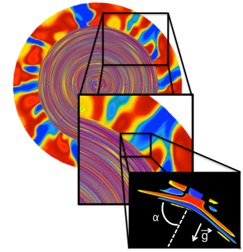
Figure 9: Zoom in the region of excitation of a wave in model ref. The plane shown is the one perpendicular to the plume of interest (blue zone in the center of the middle panel), where a St Andrew’s cross is produced (third panel). In the last panel, the radius is extended, and the background color changed to black to make the cross more apparent.

3.3 Wavefronts in 3D

We now understand how IGWs are excited by the penetration of convective plumes in the radiative zone. An interesting question could be the orientation of the plumes and the way waves propagate in the 3D sphere. Indeed, looking at Fig. 5, it seems that wavefronts of IGWs fill the whole radiative region without distinction between longitudinal and latitudinal directions. In Fig. 11, however, we show that both planes are not equivalent for propagating waves. The lefthand panel shows the radial velocity as a function of normalized radius and longitude $\varphi$ for colatitude $\theta=\pi/2$ (equatorial plane). We see convective plumes between $r=0.69$ and $0.78R_{\odot}$ that form St Andrew’s crosses as discussed in the previous section. The wavefronts are thus inclined with respect to the horizontal. In the righthand panel, we represent $\mathrm{v}_{r}$ as a function of the colatitude $\theta$ for $\varphi=0$. This time, the wavefronts are almost parallel to the horizontal. By following the transition from equatorial to polar plane, we understand that the waves are mainly excited in the region close to the equator, but then propagate throughout the whole sphere. We see later that the region of propagation of IGWs depends on their azimuthal number $m$.

Figure 10: Propagation of two gravity waves calculated by raytracing. The top panel shows a wave at the low-frequency $\omega_{1}=3\times 10^{-3}$ mHz. The ray spirals toward the center with an almost radial wavevector, i.e., $k_{h}\ll k_{r}$. In the bottom panel, a higher frequency wave with $\omega_{2}=0.2$ mHz is represented with arrows indicating the directions of $\@vec{k}$, $k_{r}$, and $k_{h}$. The scale is respected, so $k_{h}\approx\frac{1}{5}k_{r}$. Blue arrows in the top right of each panel point out the place where both waves are excited.

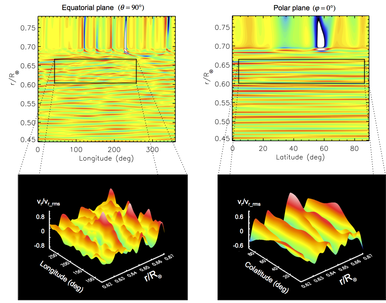
Figure 11: Form of the wavefronts in the equatorial and polar planes. Top: Contour plots of the normalized radial velocity in the equatorial (left) and polar (right) planes zoomed in the upper region of the radiative zone. Bottom: Surface plots corresponding to the region delimited by the black rectangles in the top panel that show the amplitude of the wavefronts varying with longitude (left) and colatitude (right). The velocity has been divided by its rms value at each radius, in order to visualize the form of the wavefront despite the attenuation of the amplitude.

3.4 Spectrum

We are therefore able to see low-frequency IGWs excited by convective penetration and propagating in the radiative zone. However, observing the waves in the physical space is not sufficient for characterizing them because only the largest perturbations are visible. Indeed, other waves with lower amplitudes could be excited but not directly observable.

Starting from a temporal sequence of the radial velocity field $V_{r}(r_{0},\theta,\varphi,t)$ at a given depth $r_{0}$, we successively apply a spherical harmonic transform at each time step, which gives $\hat{V_{r}}(r_{0},\ell,m,t)$, followed by a temporal Fourier transform on the whole sequence of ($\ell$,$m$) spectra. This transformation into spherical harmonics allows us to quantitatively compare our results to seismic observations and oscillation calculations, which could not be possible in 2D. We thus obtain a new field $\tilde{V_{r}}(r_{0},\ell,m,\omega)$, which can be represented as a function of $\omega$, $\ell$, and $m$. The maximum degree $\ell_{\mathrm{max}}$ is related to the horizontal resolution $N_{\theta}$ of the model (Clune et al., 1999)

$$\ell_{\mathrm{max}}\leq\frac{2N_{\theta}-1}{3}\hbox{.}$$ (20)

For models ref, therm1, therm2, and turb1, we have $\ell_{\mathrm{max}}=170$ and $\ell_{\mathrm{max}}=340$ for models turb2 and sem-lin (see Sect. 4.4) . We discuss the effect of rotation later, and for the moment, we add all contributions in $m$ quadratically in order to create a power spectrum in $\omega$ and $\ell$. This results in the following quantity:

$$E(r_{0},\ell,\omega)=\sum_{m}|\tilde{V_{r}}(r_{0},\ell,m,\omega)|^{2}\hbox{.}$$ (21)

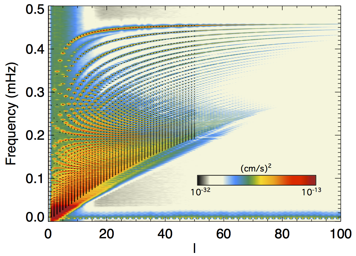
Figure 12: Energy $E$ in (cm/s)² plotted as function of the degree $\ell$ and the frequency $\omega$ at the radius $r_{0}=0.26$ $R_{\odot}$ (model ref). Ridges are visible at high frequency, tending to the maximum Brunt-Väisälä frequency (about 0.45 mHz). Black crosses represent the frequencies predicted by the oscillation code ADIPLS for order $\ell\in[1,50]$ and radial number $n\in[0,58]$. We have cut the horizontal axis to $\ell=100$ since no ridges are visible farther out.

In Fig. 12, we plot $E$ as a function of $\ell$ and $\omega$ for $r_{0}=0.26R_{\odot}$. The figure obtained looks very similar to the one predicted by linear theory (e.g., Provost & Berthomieu, 1986; Christensen-Dalsgaard, 1997). Black crosses superimposed on the colored background mark the position of the frequencies predicted by the oscillation code ADIPLS. We computed these frequencies using the ASH background state for $\ell=1$ to 50. The agreement with ASH results varies from 99% for low frequencies to 92% for high frequencies (that corresponds to lower radial order $n$). This could be because the volume of the cavity where modes are formed is submitted to slight variations during time. Indeed, the interface between convective and radiative zones is time-dependent. We estimate that this could affect the modes’ frequencies by about 1% to 3%. The BV frequency is very close to zero at this depth that limits the impact. We also consider that we measure the frequencies in ASH using finite (about 100 days) temporal sequences, and finally, nonlinear interactions and radiative effects are not taken into account in ADIPLS code and are possibly responsible for small changes in the modes’ frequencies. Modes with the same radial order $n$ - essentially given by the number of zeros in the radial direction in the eigenfunctions - form ridges, particularly visible at high frequency. As imposed by the dispersion relation (Eq. (16)) and invoked in Sect. 3.2, the maximum frequency corresponds to the maximum value of the BV frequency represented in Fig 8, i.e., $\sim$ 0.45 mHz. The modes’ frequencies are known to decrease with increasing radial order $n$. The theoretical spectrum extends to zero frequency at all degrees $\ell$, but the radial resolution of our simulation imposes an upper limit to the order $n$ (here $n_{max}\sim 58$). The richness of this spectrum proves that a large set of waves is actually excited, and not only the low-frequency IGWs visible in the real space. We then discuss the detailed properties of this spectrum in the following section.

4 Waves’ properties

The properties of internal gravity waves have been studied in detail using linear-and asymptotic theories. In this section, we show that the waves observed in our simulations verify these properties but also provide further information that is not accessible to linear theory. Here, we describe only the model ref. For the study of the waves’ frequencies, all models are equivalent. The differences lie in the amplitude of waves that are discussed in Sect. 5.

4.1 Phase and group velocities

For the moment, let us come back to the physical domain. To describe the propagation of a wave, we define the group velocity $\@vec{\mathrm{v}}_{g}=\@vec{\nabla}_{k}\omega$, the speed at which the envelope of the wave (and thus the energy) propagates through space, and the phase velocity $\@vec{\mathrm{v}}_{p}=\displaystyle\frac{\omega}{k}\@vec{\hat{k}}$, which characterizes the propagation of wavefronts (constant phases). We denote $\@vec{\hat{k}}$ as the unit vector in the direction $\@vec{k}$, and $\@vec{\nabla}_{k}\omega$ the gradient of the frequency $\omega$ as a function of the wavevector $\@vec{k}$. From Eq.(16), we can deduce the vertical and horizontal components of the group and phase velocities of a gravity wave:

$$\left\{\begin{array}[]{l}V_{\mathrm{pr}}=\displaystyle\frac{\omega}{k^{2}}k_{r}=N\left(\displaystyle\frac{k_{r}k_{h}}{k^{3}}\right)\hbox{,}\\ V_{\mathrm{ph}}=\displaystyle\frac{\omega}{k^{2}}k_{h}=N\left(\displaystyle\frac{k_{h}^{2}}{k^{3}}\right)\hbox{,}\\ V_{\mathrm{gr}}=\displaystyle\frac{\partial\omega}{\partial k_{r}}=-N\left(\displaystyle\frac{k_{r}k_{h}}{k^{3}}\right)\hbox{,}\\ V_{\mathrm{gh}}=\displaystyle\frac{\partial\omega}{\partial k_{h}}=\displaystyle\frac{N}{k}\left(1-\frac{k_{h}^{2}}{k^{2}}\right)\hbox{.}\end{array}\right.$$ (22)

A simple scalar product shows the orthogonality of $\@vec{\mathrm{V}}_{\mathrm{p}}$ and $\@vec{\mathrm{V}}_{\mathrm{g}}$, and we also notice that $V_{\mathrm{pr}}=-V_{\mathrm{gr}}$. As already presented in Sect. 3.2, Fig. 10 obtained with our raytracing code provides an illustration of the directions of $\@vec{k}$, $\@vec{\mathrm{V}}_{\mathrm{g}}$, and $\@vec{\mathrm{V}}_{\mathrm{p}}$. For the low-frequency waves visible in Fig. 5, we can measure their phase velocity by plotting the variations in radial velocity (for instance) as a function of the normalized radius for three consecutive instants (Fig. 13). The signal translates with time from inward to outward. Wavefronts are easy to locate in this figure because their propagation is mainly radial (as explained in Fig. 10). The Brunt-Väisälä frequency $N$ is a function of the radius so the phase velocity is not constant. Nevertheless, we can give an estimation of its value by measuring the mean distance travelled by the wavefronts during a given time. We find $V_{\mathrm{pr}}\approx 2\times 10^{3}$ cm/s.
Measuring the horizontal phase velocity is more difficult. Thus, we here use our raytracing code to calculate the theoretical values corresponding to the frequency $\omega_{1}=3\times 10^{-3}$ mHz. Figure 14 shows the evolution of $\@vec{\mathrm{V}}_{\mathrm{p}}$, $\@vec{\mathrm{V}}_{\mathrm{g}}$, and $\@vec{k}$ along the ray. Radial components of $\@vec{\mathrm{V}}_{\mathrm{p}}$ and $\@vec{k}$ are about two orders of magnitude higher than their horizontal parts. This is fully coherent with the almost circular spiral observed and with the asumption $k_{h}\ll k_{r}$ in the literature concerning low-frequency gravity waves ($\omega\ll N$).

Figure 13: Radial velocity fluctuations $\mathrm{v}_{r}(r,\theta_{0},\varphi_{0})$ as function of normalized radius for $\theta_{0}=35^{o}$ (top) and $\theta_{0}=75^{o}$ (bottom) represented for three consecutive instants (model ref). The longitude $\varphi_{0}=150^{o}$ is the same for both panels. The wavefronts move from the left to the right, allowing a radial phase velocity $V_{\mathrm{pr}}\approx 2\times 10^{3}$cm/s to be measured, independent of $\theta_{0}$ and the same order of magnitude than the one calculated for a ray at $\omega_{1}=3\times 10^{-3}$ mHz (see Fig. 14).

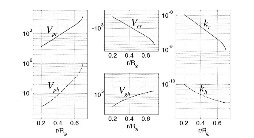
Figure 14: Components of phase velocity, group velocity, and wavevector computed by raytracing for the frequency $\omega_{1}=3\times 10^{-3}$ mHz. The corresponding raypath is shown in the top panel of Fig. 10. The velocities are expressed in cm/s and the wavevector components in cm^-1. We observe that the ratio between $k_{r}$ and $k_{h}$ is about $10^{2}$ which explains the almost circular spiral observed in Fig. 10.

4.2 Spectrum

The low-frequency waves that we see in real space are not the only ingredients of the excited spectrum. We have given an overview of the richness of this spectrum in Sec. 3.4. We now propose a more detailed analysis.

4.2.1 Temporal and spatial dependencies

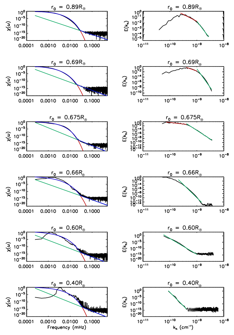
Figure 15: Decomposition of the spectrum $E(r_{0},k_{h},\omega)$ of model ref into its temporal and spatial dependencies. The best fit for $\chi(\omega)$ is a combination of a Gaussian-like and a Lorentzian-like functions since $E(k_{h})$ decreases as $k_{h}^{-\eta}$ with $\eta$=5-7.

We recall that the quantity studied here is given by Eq. (21). Since $E(r_{0},\ell,\omega)$ depends on both $\ell$ and $\omega$, we would like to be able to distinguish between these two dependencies. The frequency $\omega$ corresponds to the temporal variations. We thus introduce the horizontal wavevector, $k_{h}=\displaystyle\frac{\sqrt{\ell(\ell+1)}}{r}$, to characterize the spatial variations. A first method should be to choose a value of $\omega$ to study the variations of $E$ with $k_{h}$ and vice versa. That is the method employed by Belkacem et al. (2009) to obtain the function $\chi(\omega)$ with a wavenumber $k_{h0}$ corresponding to the maximum of energy. The disadvantage of this method is that it does not consider the whole spectrum. For this reason, we chose to follow the idea of Rogers et al. (2013) by computing a singular value decomposition (SVD) of $E(r_{0},k_{h},\omega)$. The concept of the SVD is to decompose $E$ into its separable part and a leftover part such that

$$E(r_{0},k_{h},\omega)=c_{1}E(k_{h})\chi(\omega)+\sum_{i>1}c_{i}E_{i}(k_{h},\omega)\hbox{.}$$ (23)

Of course, this is meaningful only if the initial function $E$ is separable. We compute this decomposition for several depths $r_{0}$. In the convective zone ($r_{0}\geq 0.69$ $R_{\odot}$ if we take the overshoot region into account), the ratio $c_{1}/\sum_{i}c_{i}$ characterizing the separability of $E(r_{0},k_{h},\omega)$ varies between 60% and 66% and is superior to 84% in the radiation zone. Figure 15 shows the result of these calculations where we have superimposed the best fit for each curve. In the convection zone, gravity waves are evanescent so the spectrum is mainly a turbulence spectrum associated with thermal convection. The chosen fit is a combination of a Gaussian-like function

$$\mathcal{G}(\omega)=\frac{1}{\sqrt{\pi}\omega_{G}}\exp\left({-\left[\frac{\omega}{\omega_{G}}\right]^{\alpha_{G}}}\right)\hbox{,}$$ (24)

and a Lorentzian-like function

$$\mathcal{L}(\omega)=\frac{2}{\pi\omega_{L}}\left[\frac{1}{1+\left(\frac{\omega}{\omega_{G}}\right)^{\alpha_{L}}}\right]\hbox{,}$$ (25)

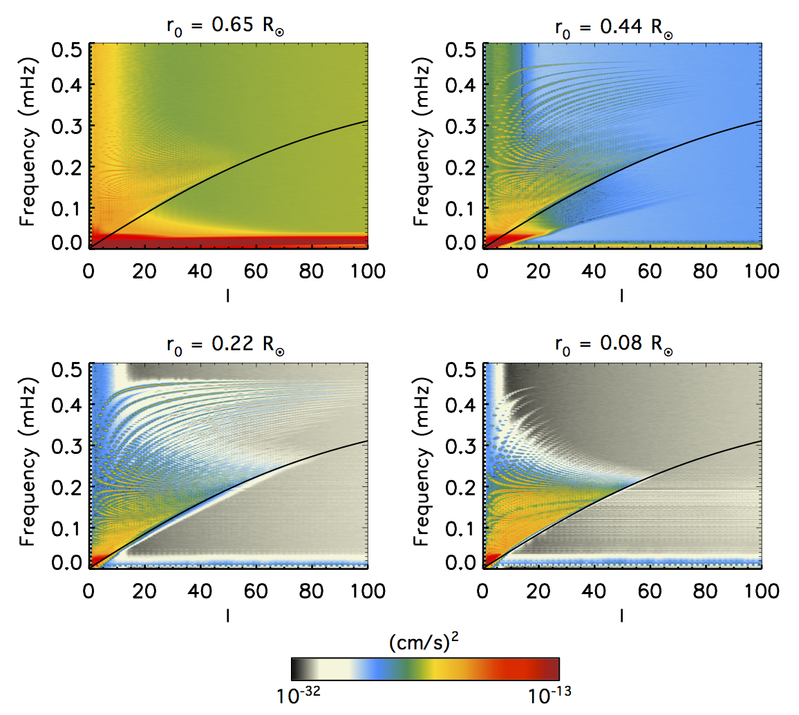
Figure 16: Variation in the spectrum shape as function of depth $r_{0}$ (model ref). The black line marks the last resolved ridge $n=58$ common to all depths. We have volontarily cut the horizontal axis to $\ell=100$ to show the part where ridges are the most visible and used the same color table for the four depths, although the minimum and maximum amplitudes vary greatly. In particular, the change in the background color shows the increase in the background noise when reaching the excitation zone ($r_{0}=0.65R_{\odot}$) and then entering the convective region.

where $\omega_{G}=3\beta$ and $\omega_{L}=\beta/3$. The parameters vary with $r_{0}$ in the range $\alpha_{G}\in$ [0.67,0.8], $\alpha_{L}\in$ [5,6], and $\beta\in$ [0.06,0.13]. For the eddy-time function $\chi(\omega)$, we retrieve the results found by Belkacem et al. (2009) in the convective zone, showing that the best fit is not a pure Gaussian function as used in Goldreich et al. (1994), but rather a combination with a Lorentzian-like function. However, we notice that we had to increase $\alpha_{L}$ from 2 to 5-6 to fit the strong slope formed by $\chi(\omega)$ at high frequency.
These results are similar if we apply the SVD to the more turbulent models turb1 and turb2. Because Belkacem et al. (2009) studied spectra coming from a purely convective shell, the difference may be due to the coupling with the radiative interior. This fit remains approximatively correct in the radiative zone, although the energetical peaks relative to gravity waves make the spectrum more noisy at high frequency. For $E(k_{h})$, we also observe a modification of the form when passing from convective to radiative interior. For $r_{0}>0.66R_{\odot}$, we fit the curve with two straight lines. The red line (left) corresponds to the slope $k_{h}^{-5/3}$ of a Kolmogorov turbulence spectrum. This result agrees with Samadi et al. (2003). For higher horizontal wavenumbers, we fit the curve with a second straight line (green) that is much more inclined ($k_{h}^{-5}$ to $k_{h}^{-7}$). This result seems to be closer to the one presented by Rogers et al. (2013). In the radiative zone, the spectrum is no longer turbulent, and only the strongest slope remains. To conclude, the SVD reveals that the temporal part of the spectrum behaves more like a Lorentzian, whereas its spatial part have a power that decreases as $k_{h}^{-5}$ to $k_{h}^{-7}$.

4.2.2 Variation with depth

We now have a look at the differences between spectra calculated at different depths $r_{0}$. We recall that the spectrum shown in Fig. 12 was taken at $r_{0}=0.26R_{\odot}$. In Fig. 16, we display four spectra calculated with the same temporal sequence of model ref. The first one is taken near the region of excitation ($r_{0}=0.65R_{\odot}$), the last one near the center ($r_{0}=0.08R_{\odot}$), and the two others in the middle of the radiative zone ($r_{0}=0.44R_{\odot}$ and $r_{0}=0.22R_{\odot}$). We do not show the convective zone since no modes are visible there. It is clear that the spectrum’s aspect is different depending on the depth. First of all, we notice that a common feature between all these spectra is the inferior limit underlined by a black line. It is situated exactly at the same place in all spectra and corresponds to the ridge number $n=58$. Since the order $n$ represents the number of nodes of the radial eigenfunctions (see Sect. 4.3.1), we can understand that this boundary is due to the radial resolution of our model. At 0.65$R_{\odot}$, only the low-frequency part of the spectrum is visible. If we move deeper in radius, higher frequencies appear. For $r_{0}=0.44R_{\odot}$, there is a region that looks different, under the black line. The energy in this region does not form peaks that are regularly spaced in period, such as g-modes should. Consequently, we interpret this region as propagating gravity waves that do not form g-modes. This zone reduces and disappears when we move down in depth reinforces this hypothesis since it corresponds to the action of the radiative damping on these waves (discussed in Sect. 5.2).

4.3 g-modes

Until now, we have looked at the overall shape of the spectrum, considering both propagative and standing IGWs. In this section, we concentrate on the high-frequency part of the spectrum corresponding only to g-modes. They are identifiable by their radial order $n$ defined by the number of nodes of their eigenfunction.

4.3.1 Period spacing and eigenfunctions

We first focus on the behavior of $E$ for a given order $\ell$. One of the main asymptotic properties of g-modes - used to detect their signatures in the Sun (Garcia et al., 2007) and stars (Bedding et al., 2011) - is that they are supposelly equally spaced in period (e.g., Aerts et al., 2010). To check this property, we represent the variations in $E(r_{0},\ell,\omega)$ in Fig. 17 as a function of $\omega$ and $P=1/\omega$ for $\ell$=1, 2, and 3. We volontarily limit the frequency to the range [0.05,0.30] mHz for $\ell$=1, and [0.05,0.45] mHz for $\ell$=2 and 3 to focus only on well defined peaks corresponding to radial orders $n\leq 20$. The bottom panel represents the Fourier transform of the period spectrum, and we observe that a main peak appears, indicating the value of $\Delta P_{\ell}$, the period spacing between modes. We find $\Delta P_{1}=37.1$ min, $\Delta P_{2}=21.2$ min, and $\Delta P_{3}=14.8$ min.

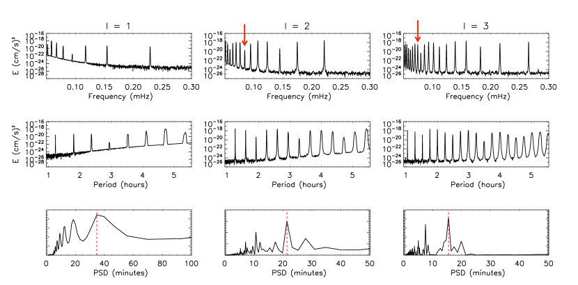
Figure 17: Top and middle: Spectrum of gravity waves for $\ell=1,2,3$ as function of frequency and period. Bottom: Fourier transform of the middle spectrum that shows the constant period spacing between peaks. We find $\Delta P_{1}=37.1$ min, $\Delta P_{2}=21.2$ min, and $\Delta P_{3}=14.8$ min as pointed out by vertical red dotted lines.

The asymptotic theory predicts that $\Delta P_{\ell}$ must be given by

$$\Delta P_{\ell}=\frac{\pi}{\sqrt{\ell(\ell+1)}\displaystyle\int_{r_{1}}^{r_{2}}\displaystyle\frac{N}{r}dr}\hbox{,}$$ (26)

where $r_{1}$ and $r_{2}$ are the turning points defined by $N(r_{1})=N(r_{2})=\omega$ (e.g., Christensen-Dalsgaard, 1997). We compare our measures to the values given by Eq. (26) for several $\ell$. By taking for $N$ the profile defined in ASH and represented in Fig. 8, we obtain on average agreement of about 5% between the theoretical and the measured values. This small difference is due, on one hand, to the error made by measuring $\Delta P_{\ell}$ with a finite time sequence and on the other, from the fact that Eq. (26) has been obtained assuming $n\gg\ell$. As recall above, Garcia et al. (2007) have used the equally spacing between modes to detect their signature in the GOLF data from the Sun. For $\ell$=1, they found a peak corresponding to $\Delta P_{1}$ located between 22 and 26 minutes. For $\Delta P_{2}$, they were expecting 9-15 minutes and 5-11 minutes for $\Delta P_{3}$. In Eq. (26), we see that $\Delta P_{\ell}$ is inversely proportional to $\displaystyle\int_{r_{1}}^{r_{2}}\displaystyle\frac{N}{r}dr$. Then, we can show that 60% of the total value of this integral is built on the value of $N$ in the inner 0.2 $R_{\odot}$ (Brun et al., 1998; Alvan et al., 2012). Consequently, a slight difference in the BV profile between our model and the one used by Garcia et al. (2007) can easily explain the observed bias.

As shown in Sect. 4.2.2, we are able to calculate the spectrum at different depths. To visualize the radial evolution of some g-mode amplitudes, we represent a map of the energy $E(r,\ell=5,\omega)$ Fig. 18 as a function of the normalized radius $r/R_{\odot}$ and the frequency $\omega$. This figure was obtained by calculating the spectrum for each radial point. We can count the number $n$ of nodes in the radial eigenfunctions and see that it increases with decreasing frequencies. The signal is projected on the bottom of the figure, which allows to precisely see the distribution of the nodes as a function of the radius and the frequency. The bottom panels provide a comparison between the eigenfunctions in ASH and in ADIPLS for three different values of $n$.

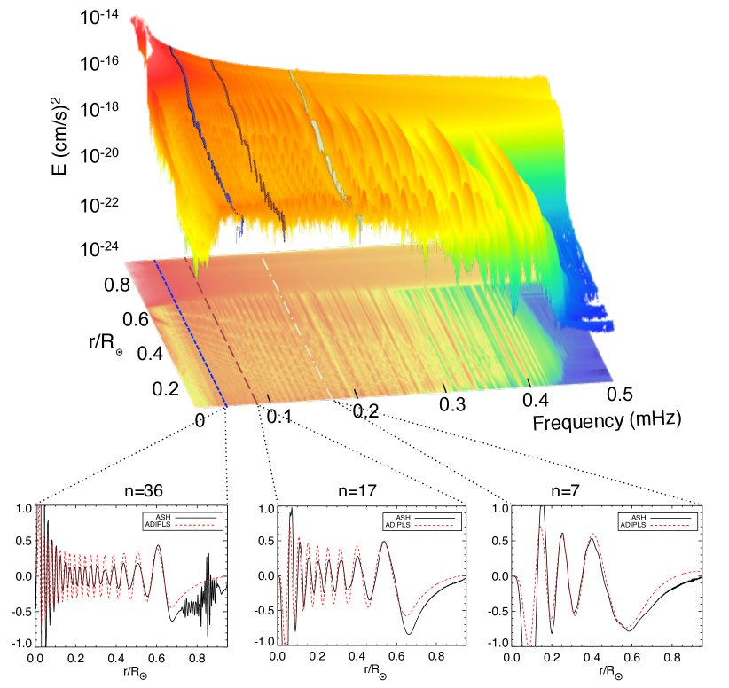
Figure 18: Top: Energy $E$ as a function of the normalized radius and frequency for the order $\ell$=5 (model turb2). Bottom: Extraction of three normalized eigenfunctions corresponding to $n=36$, $n=17$, and $n=7$. Their positions in the top panel are indicated by blue dashed, red long dashed and green dot-dashed lines. The eigenfunctions computed by the oscillation code ADIPLS are represented by red dotted lines.

4.3.2 Rotational splitting

Until now, we have put aside the effects of rotation by summing over all the $m$ components of a given $\ell$ mode. Without rotation, although $m$ modes are not located at the same place ($m$=0 lies in the meridional plane and the more high $|m|$ the more inclined the plane), the frequencies are degenerated. That is to say that modes identified by the same pair ($\ell$,$n$), but different $m$ are merged in the same peak in the spectrum. But we do not forget that all models presented in this paper rotate at the solar rotation rate $\Omega_{\odot}$ (see Fig. 4). To look at rotational effects we thus need to distinguish one $m$ component from one another. One must first establish the difference between prograde (propagating in the direction of rotation) and retrograde waves. Thus, rotation increases the phase speed of prograde waves and decreases the one of retrograde waves. This results in a separation of their frequencies. Figure 19 is the superposition of peaks with same values of $\ell$, but values of $m$ vary between $-\ell$ and $+\ell$. We recall that the energy $E$ is obtained from the radial velocity $V_{r}(r_{0},\theta,\varphi,t)$ thanks to a spherical harmonic transform followed by a temporal Fourier transform. To obtain negative values of $m$, we took the temporal Fourier transform of $\hat{V}_{r}^{*}(r_{0},\ell,m,t)$, which is the complex conjugate of $\hat{V}_{r}(r_{0},\ell,m,t)$ (see Sect. 3.4). We observe that the peaks move from left to right as $m$ increases. We thus retrieve the phenomenon called rotational splitting (e.g., Aerts et al., 2010) that allows asteroseismologists to reconstruct the internal rotation profile of stars (Deheuvels et al., 2012).

The theory of stellar oscillations (e.g., Christensen-Dalsgaard, 1997) predicts that the frequency splitting must be given by

$$\delta_{n\ell m}=m\beta_{n\ell}\displaystyle\int_{0}^{R_{\odot}}K_{n\ell}(r)\Omega(r)\mathrm{d}r\hbox{,}$$ (27)

where

$$K_{n\ell}(r)=\frac{\left(\xi_{r}^{2}+L^{2}\xi_{h}^{2}-2\xi_{r}\xi_{h}-\xi_{h}^{2}\right)r^{2}\bar{\rho}}{\displaystyle\int_{0}^{R_{\odot}}\left(\xi_{r}^{2}+L^{2}\xi_{h}^{2}-2\xi_{r}\xi_{h}-\xi_{h}^{2}\right)r^{2}\bar{\rho}\mathrm{d}r}\hbox{,}$$ (28)

and

$$\beta_{n\ell}=\frac{\displaystyle\int_{0}^{R_{\odot}}\left(\xi_{r}^{2}+L^{2}\xi_{h}^{2}-2\xi_{r}\xi_{h}-\xi_{h}^{2}\right)r^{2}\bar{\rho}\mathrm{d}r}{\displaystyle\int_{0}^{R_{\odot}}\left(\xi_{r}^{2}+L^{2}\xi_{h}^{2}\right)r^{2}\bar{\rho}\mathrm{d}r}\hbox{,}$$ (29)

are functions of the radial and horizontal displacements ($\xi_{r}$ and $\xi_{h}$) and of the reference density $\bar{\rho}$, and $L^{2}=\ell(\ell+1)$. Moreover, the rotational kernel $K_{n\ell}$ is unimodular, i.e.,

$$\int_{0}^{R_{\odot}}K_{n\ell}(r)\mathrm{d}r=1\hbox{.}$$ (30)

For high-order g modes, we can neglect the terms containing $\xi_{r}$, so that

$$\beta_{n\ell}\approx 1-\frac{1}{\ell(\ell+1)}\hbox{,}$$ (31)

and for a uniform rotation $\Omega_{S}$ (in the radiative zone), we obtain

$$\delta_{n\ell m}=m\beta_{n\ell}\Omega_{S}\hbox{.}$$ (32)

Finally, in the frame rotating with the star, it becomes

$$\delta_{n\ell m}=-m(1-\beta_{n\ell})\Omega_{S}\hbox{.}$$ (33)

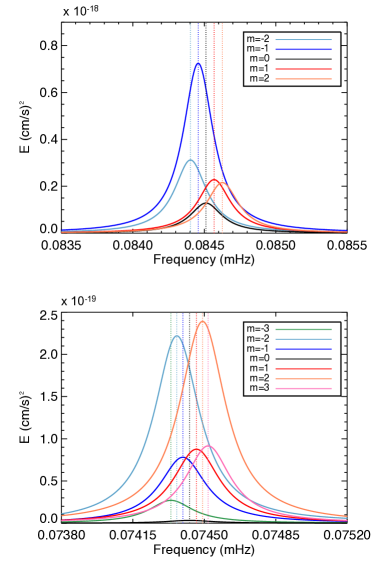
Figure 19: Rotational splitting for $\ell=2$ and $-2<m<2$ (top) and $\ell=3$ and $-3<m<3$ (bottom). The chosen frequencies are identified by red vertical arrows in Fig. 17. Here, the peaks have been fitted with a Lorentzian function to determine the position of their maximum precisely.

The usual way to use this relation is to deduce the rotation rate $\Omega_{S}$ from the measure of $\delta_{n\ell m}$. Here, since we already know the value of $\Omega_{S}=\Omega_{\odot}$, we can evaluate the precision of this method. In Fig. 20, we represent the values of $\Omega_{S}$ obtained by inserting different measures of $\delta_{n\ell m}$ in Eq. (33). As expressed by Eq. (30), these values do not depend on the depth at which we extract the spectrum. We observe that we approach the real solar rotation rate imposed in the simulation ($2.6\times 10^{-6}$ rad/s) when $n$ increases. Indeed, although the convective zone is submitted to a differential rotation, IGWs are not sensitive to it because they do not propagate into this zone. This result confirms that Eq. (33) is mostly valid for asymptotic modes. Unfortunately, the more we increase $n$, the more the frequency decreases, so peaks get very close to each other. For this reason, the identification of peaks corresponding to the same couple ($\ell$,$n$) becomes imprecise, if not impossible, for very high $n$ and we have to stop around $n=35$. In spite of that, the convergence is quick enough to estimate the rotation with an accuracy of 30% from $n=10$ (corresponding to frequencies in the range [0.05,0.1] mHz for $\ell\sim 2-4$, which can be observed in stars) knowing that the rotation rate $\Omega_{S}$ is mostly underestimated by this method. To increase the precision to 5%, we have to look at modes with $n>25$ that corresponds to frequencies around 0.01 mHz.

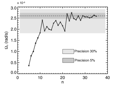
Figure 20: Estimation of the rotation rate from measuring the rotational splitting for $\ell$=3. The same tendency is obtained for other values of $\ell$. Two gray zones indicate the precision of the measure with respect to the right rotation rate that is imposed. We obtain less than 5% error for $n>$ 30.

Another interesting piece of information supplied by Fig. 19 is the asymmetry of amplitude between prograde and retrograde modes. It is clear here that the usual assumption of energy equal distribution is not verified (Belkacem et al., 2009) and that one should take this bias into accound in asteroseismic and stellar evolution studies. We also notice in both panels that the $m=0$ peak is much lower than the other ones. For $\ell=3$, $m=0$ is hardly visible because it is very close to the horizontal axis. In contrast, higher peaks correspond to higher $m$. As explained above, in a spherically symmetrical star, IGWs propagate in planes inclined with respect to the meridional plane as a function of $m$. We thus understand that the most energetic modes lie in planes close to the equatorial plane, and we might be more able to detect them in this area.

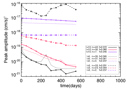
Figure 21: Evolution of the peak’s amplitude as a function of time. High-frequency waves (violet) have a lifetime much greater than 550 days since their amplitude does not vary over this time interval. Intermediate-frequency waves (red) are damped along their propagation and for low-frequency waves (black) their amplitude sometimes increases suddenly, due to a re-excitation. The legend indicates the values of ($\ell$,$n$) and the corresponding frequency $f$ in mHz for each curve.

4.3.3 Lifetime

The knowledge of g-mode lifetimes is very important for detecting them in the Sun. Goldreich & Kumar (1990) find mode lifetimes of about 106 years, while Appourchaux et al. (2010) give about 1 million years. Thus a large incertainty remains in the literature about this value. The standard method for obtaining the lifetime of modes is the measure of the half width at half maximum (HWHM) of the peaks. This implicitly supposes that the time series used to calculate the spectrum are much longer than the lifetime. In this work, a timescale of several hundred years is out of reach because we have to deal with a time step of about 100s. Our maximum currently availabe time series is about 550 days. To skirt the problem, we have cut this main sequence into several consecutive subsequences (11 times 50 days) and measured the amplitude of some peaks in each subsequence. Figure 21 represents these amplitudes as a function of time. Three regimes are identifiable. High-frequency waves are almost constant in amplitude or slightly decreasing. This shows that the lifetime of high-frequency modes is indeed much greater than 550 days. Intermediate-frequency waves are damped (thermal effects) along their propagation.
A comparison shows a disagreement between this temporal damping and linear theoretical predictions. Indeed, when using the linearized equations for the gravity waves propagation (e.g., Zahn et al., 1997), the wave’s amplitude is expected to decrease as predicted by Fritts et al. (1998)

$$e^{-\displaystyle\kappa_{r}\displaystyle\frac{k_{h}^{2}}{2}\frac{N^{2}}{\omega^{2}}t}\hbox{,}$$ (34)

which gives a much steeper slope than the one observed in Fig. 21. We discuss the role played by nonlinearities in mitigating the damping effects in Sect. 5.2. Finally, low-frequency waves seem to be re-excited during this temporal window since their amplitude increases abruptly at a some instants, for example at $t=250$ days. This excitation may be due to the arrival of a new plume exciting a wave at the same frequency. This would be coherent with our observations of Sect. 3.2 showing that convection excites high-amplitude low-frequency waves. The other possibility for explaining this re-excitation process could be related to the nonlinear interactions between two other waves (cf. Sect. 4.4).

Figure 22: Comparison between fully nonlinear model turb2 in panels (a) and (c) and semi-linear model sem-lin in panels (b) and (d). The quantity represented is the normalized radial velocity. Both top panels are equatorial slices where we see the outer convective region (red/blue tones denote positive/negative values). The cross shape visible in the radiative zone in top left panel is a Moiré pattern. In the bottom panels, we have zoomed in the upper part of the radiative zone to highlight the departure of wavefronts from the base of plumes. We can measure the angle formed by the wavefronts in both situations and deduce that nonlinear interactions favor low-frequency waves.

4.4 Nonlinear wave interactions

In this section, we compare the previous results - obtained thanks to a nonlinear resolution of the hydrodynamical equations Eq. (4) and (Appendix A: Inner boundary conditions) - and a model called sem-lin where we have set the nonlinear terms in the radiative region to zero, as inspired by a similar approach in Rogers & Glatzmaier (2005a). We multiplied the nonlinear terms by a function equal to one if $r>0.73$R_⊙, to zero if $r<0.71$R_⊙, and decreasing linearly from 1 to 0 between these points. Except for this filter, the model sem-lin is identical to turb2. We activated the filter at time $t_{0}$ when the model is relaxed and stable. Figure 22 compares the dynamics in the radiative interiors of both models. We have represented the normalized radial velocity $v_{r}/v_{rms}$ at colatitude $\theta=\pi/2$ (equatorial plane) as a function of longitude $\varphi$ and normalized radius. Lefthand panels (a) and (c) correspond to the fully nonlinear model turb2 and righthand panels (b) and (d) to the model sem-lin. We observe in (b) that the wavefronts are much more inclined, looking like the high-frequency ray represented in the bottom panel of Fig. 10. We thus retrieve the same result as Rogers & Glatzmaier (2005a) in their 2D simulations. In panels (c) and (d), we have zoomed in the interface between the convective and radiative zones in order to measure the angles formed by the wavefronts. Again, it is clear that in the nonlinear case, plumes excite very low-frequency waves with wavefronts almost horizontal, as discussed in Sect. 3.2. For example, we measure $\alpha\approx 80^{o}$ at $r\approx 0.65R_{\odot}$, which gives $\omega=0.036$ mHz according to Eq. (18). In panel (d), however - corresponding to the semi-linear model sem-lin - the St Andrew’s crosses are much more pronounced. In the figure shown here, we can measure three angles $\beta\approx 55^{o}$, $\gamma\approx 22^{o}$, and $\delta\approx 45^{o}$, which correspond to frequencies 0.15 mHz, 0.19 mHz, and 0.14 mHz respectively. We could explain these observations by considering the rules governing the wave-wave interactions. As shown in the interaction diagram (Fig. 23) , there are four possible combinations for two waves to excite a third one (e.g., Müller et al., 1986). Wavevectors are vectorially added, so the two possible horizontal wavevectors are $\@vec{k}_{h3}=\@vec{k}_{h1}+\@vec{k}_{h2}$ and $\@vec{k}_{h3}=\@vec{k}_{h1}-\@vec{k}_{h2}$. The waves with the biggest wavenumber is rapidly damped and only the one with the smallest wavenumber remains. Since the frequency is linked to the wavenumber by Eq. (16), we understand that nonlinear interactions favor low frequencies.

5 Waves’ amplitude and energy

In this paper, we wish to discuss two important questions concerning solar gravity waves: their precise frequencies and their amplitudes. In this section, we analyze the energetical aspects of the spectrum.

5.1 Energy transfer from convective zone to waves

First of all, we have seen in Sec. 3.1 that convective plumes are slowed down by buoyancy when they enter the radiative region and that a part of their kinetic energy is converted into gravity waves. A long series of papers attempted to quantify the excitation of gravity waves by convective penetration (Press, 1981; Zahn, 1991; Andreassen et al., 1992; Andersen, 1994; Schatzman, 1996; Talon & Charbonnel, 2003). In particular, Andersen (1994) evaluates the energy density in the waves at about 0.1% of the typical kinetic energy density in the convective zone. We used the same method by comparing the kinetic energy density in the convection zone at 0.73$R_{\odot}$ with the energy of gravity waves at 0.6$R_{\odot}$. For a given value of $\ell$, we thus define a transmission rate $T_{\ell}$ as

$$T_{\ell}(\omega)=\frac{E(r_{0}=0.73R_{\odot},\ell,\omega)}{E(r_{0}=0.6R_{\odot},\ell,\omega)}\hbox{.}$$ (35)

We plot $T_{\ell}$ for $\ell=$ 2, 8, 13 and 18 in the top panel of Fig. 24. For $\ell$=2 and $\ell$=8, we find a transmission rate that is close to the one predicted by Andersen (1994), with a main peak at 0.21%. The transmission rate is lower for higher values of $\ell$ and becomes very small for $\ell$=18. These results are unchanged by choosing other depths than 0.73$R_{\odot}$ and 0.6$R_{\odot}$, and by staying above and below the tachocline. We thus deduce that the convective kinetic energy is mainly distributed to low orders $\ell$ and orders $n$ less than ten corresponding to the range of frequencies $[0.10,0.25]$ mHz.

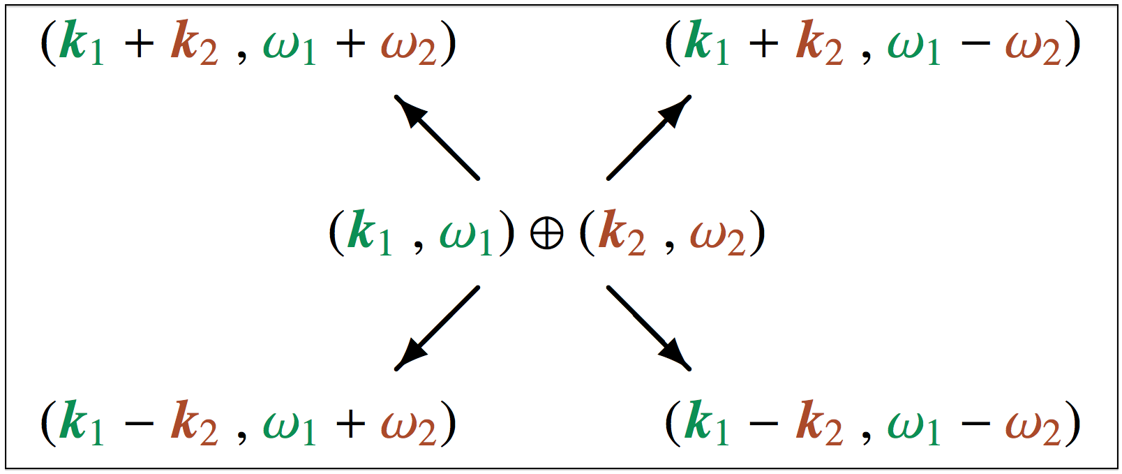
Figure 23: Diagram showing the possibilities for two waves $(\@vec{k}_{1},\omega_{1})$ and $(\@vec{k}_{2},\omega_{2})$ to interact and give birth to a third wave.

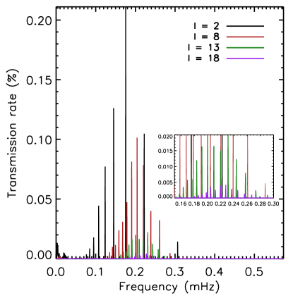
Figure 24: Transmission of energy from convective to radiative zone for different values of $\ell$. We retrieve the estimation of 0.1% given in previous works for the most visible peak, but the transmission rate decreases rapidly when increasing $\ell$.

Figure 25: Fraction of the total luminosity converted into waves. At the base of the convecting zone, the luminosity carried by waves is about 0.4% $L_{\odot}$, which is coherent with the amount of energy transmitted from convection to waves (Fig. 24).

But it is also interesting to estimate the energy flux carried by IGWs with respect to the total luminosity. Several formula have been used to calculate this flux. The first one is the flux associated with the pressure fluctuations (acoustic flux) (Lighthill, 1978; Mathis, 2009),

$$\mathcal{F}_{p}=<\overline{V_{r}P}>\hbox{.}$$ (36)

It is directly linked to the angular momentum flux that characterizes the deposit (prograde) or extraction (retrograde) of angular momenum by waves (Zahn et al., 1997). Then, when $\omega_{c}\ll N$, one defines the total energy flux $\mathcal{F}_{W1}$ carried by IGWs by

$$\mathcal{F}_{W1}\propto\frac{\omega_{c}}{N}\mathcal{F}_{c}\hbox{,}$$ (37)

where $\omega_{c}$ is the convection frequency and $\mathcal{F}_{c}$ the convective energy flux (Goldreich et al., 1994; Garcia Lopez & Spruit, 1991; Kiraga et al., 2003), and $\mathcal{F}_{W1}$ and $\mathcal{F}_{p}$ are theoretically equal. In our case, because the enthalpy flux is nearly zero in the radiative zone (see flux balance in Fig. 1), we take the maximum value for $\mathcal{F}_{c}$ in the convective zone. Moreover, for the model ref, we measure $\omega_{c}\approx$ 15 days, which verifies $\omega_{c}\ll N$ a posteriori. Finally, we consider the flux $\mathcal{F}_{W2}$ given by Zahn et al. (1997); Kiraga et al. (2003) as

$$\mathcal{F}_{W2}=\int_{\omega_{c}}^{N}\int_{k_{h}}\rho\frac{E(k_{h},\omega)}{k_{h}\omega}V_{\mathrm{gr}}(k_{h},\omega)dk_{h}d\omega\hbox{,}$$ (38)

where$V_{\mathrm{gr}}(k_{h},\omega)$ is the group velocity

$$V_{\mathrm{gr}}(k_{h},\omega)=\frac{\sqrt{N^{2}-\omega^{2}}}{N^{2}}\frac{\omega^{2}}{\sqrt{\ell(\ell+1})}r\hbox{,}$$ (39)

and $E(k_{h},\omega)$ the quantity defined by Eq. (21). We plot in Fig. 25 the comparison between those three fluxes - $\mathcal{F}_{p}$, $\mathcal{F}_{W1}$ and $\mathcal{F}_{W2}$ - converted into luminosity - $L_{p}$, $L_{W1}$, and $L_{W2}$ - and divided by the solar total luminosity $L_{\odot}$. The righthand part of the figure is a zoom in the top region of the radiative zone. The linear vertical scale shows that the three luminosities are comparable around $4\times 10^{-3}L_{\odot}$ in the region of excitation of IGWs. However, the acoustic flux drops rapidly and becomes extremely small for $r<0.68R_{\odot}$. The lefthand panel of Fig. 25 shows the two remaining fluxes in the whole radiative zone with a logarithmic vertical scale. We see that $\mathcal{F}_{W1}$ and $\mathcal{F}_{W2}$ remain similar, decreasing from $10^{-3}$ to $10^{-5}$ $L_{\odot}$. Thus, it seems that we find a consistency between the percentage of the solar luminosity carried by IGWs at the beginning of their propagation and the energy transmitted from convection to waves.

5.2 Spatial radiative damping

Gravity waves are damped during their propagation. According to Zahn et al. (1997), the amplitude of a gravity wave propagating in a non adiabatic medium is damped by a factor $e^{-\tau/2}$ where

$$\tau\left(r,\ell,\omega\right)=\left[\ell(\ell+1)\right]^{\frac{3}{2}}\int_{r}^{r_{\rm CZ}}\kappa\frac{N^{3}}{\omega^{4}}\frac{\mathrm{d}r^{\prime}}{r^{\prime 3}}\hbox{.}$$ (40)

Here we take $r_{CZ}=0.69R_{\odot}$, the radius where waves are excited (i.e., at the interface between convective and radiative zones). That formula was obtained in the linear regime and under the assumption $\omega\ll N$. To compare this prediction with our simulation, we take $E_{0}(\omega)=E(r=0.69R_{\odot},\ell=2,\omega)$ as a starting amplitude. We then look at the evolution with depth of this initial amplitude by taking

$$E_{\mathrm{damp}}(r,\omega)=E_{0}(\omega)\times e^{-\tau(r,2,\omega)}\hbox{.}$$ (41)

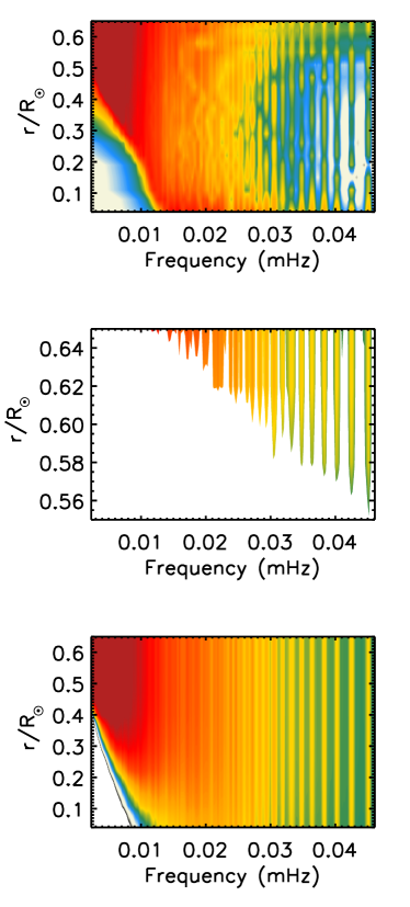
Figure 26: Comparison of simulated data with the theoretical radiative damping. Top: Spectrum obtained in the simulation (model ref, $\ell$=2). Middle: Effect of a radiative damping with the theoretical coefficient $1/\omega^{4}$. The initial amplitude is the same as in the upper panel. Bottom: Effect of radiative damping with $1/\omega^{3}$.

We represent $E_{\mathrm{damp}}$ as a function of $r/R_{\odot}$ and $\omega$ in Fig 26. The top panel shows the spectrum obtained by ASH. We can understand this figure as Fig. 18 seen from above (top panel). The difference is the narrow horizontal range, because the maximum frequency here is $0.045$ mHz $=N_{\mathrm{max}}/10$ to respect the hypothesis $\omega\ll N$. The vertical lines correspond to eigenfunctions, particularly visible on the right, and when frequency decreases, the modes become closer and closer. This top panel is taken as a reference in this discussion. The middle panel represents $E_{damp}(r,\omega)$ with $\tau$ calculated with Eq. (40). The profiles of $\kappa$, $\nu$, and $N$ are those presented in Sect. 2. We observe that the amplitude drops much faster than in the top panel. In the bottom panel, however, we have calculated the damping rate by replacing $\omega^{4}$ in Eq. (40) by $\omega^{3}$. The attenuation obtained is much more in accordance with the one predicted by the simulation. The same behavior has been observed by Rogers et al. (2013) in their 2D nonlinear simulations. We suspect that the nonlinear interactions between waves explain this difference between simulations and theory. Of course, we do not attempt here to redefine the formulation of the damping rate, just giving a simple trend with $\omega$.

To test this hypothesis, we use the model sem-lin described in Sect. 4.4. The wave spectra obtained are represented in Fig. 27 for two depths, $r_{0}=0.65R_{\odot}$(top) and $r_{0}=0.44R_{\odot}$(bottom). The detailed study of these results and the characterization of nonlinear interactions will be the object of a forthcoming paper. Here, the point of interest lies in the fact that the amount of energy visible in the top spectra at low frequency has totally disappeared in the bottom one. By measuring the damping rate with the same method as in Fig. 26, we obtain good agreement with a coefficient ${1}/{\omega^{3.6}}$ in Eq. (40) instead of ${1}/{\omega^{4}}$. Although we do not retrieve the predicted behaviour exactly, we are clearly closer than with the fully nonlinear model. The conclusion here is that wave-wave and/or wave-fluid nonlinear interactions play a very important role, which seems to be weighed against the linear radiative damping. Since thermal damping is one of the processes (with for instance corotation resonances and wave breaking) responsible for the angular momentum transport by IGWs in stars, this result has to be considered in, for example, stellar evolution codes that modeled this transport (Charbonnel et al., 2013; Mathis et al., 2013).

Figure 27: Spectra obtained with a 40-day sequence of model sem-lin at $r_{0}=0.65R_{\odot}$ (top panel) and $r_{0}=0.44R_{\odot}$ (bottom panel). Although the horizontal $N_{\theta}=512$ resolution of this model allows reaching $\ell_{\mathrm{max}}=340$ (see Eq. (20)), we have cut the horizontal axis to $\ell=170$ to focus on the difference between both spectra. At low frequency, the waves visible at $r_{0}=0.65R_{\odot}$ have been totally damped at $r_{0}=0.44R_{\odot}$.

5.3 Sensitivity to physical parameters

The last remaining question concerns the amplitude of g-modes in the radiative zone, but also at the surface of the Sun. Thus, we finish this paper by comparing the different models introduced in Sect. 2.4 and the corresponding IGWs’ amplitudes. In the top panel of Fig. 28, we show the rms radial velocities as a function of the normalized radius for each model. We clearly see the drop of velocity at the interface between radiative and convective zones, around $0.7R_{\odot}$. Moreover, as expected by the choice of the diffusivity coefficients and by the observation of the overshoot region (see Sect. 3.1), turb2 (violet) is the model with the highest rms velocity in the radiative zone. Then comes turb1 (blue), ref (black), therm2 (red), and therm1 (orange). The order of these curves is directly related to the values of the thermal diffusivities $\kappa$ (see Fig. 1).

For each model, we have calculated a spectrum at $r_{0}=0.66R_{\odot}$ and reported in the bottom panel of Fig. 28 the amplitudes in $cm/s$ of the highest and lowest peaks (black diamonds) of modes ($\ell$=1,2,3 and $n$=1-10). These modes are the ones identified in Sect. 5.1 as the most excited by the convection. They are thus the best candidates for a possible detection at the surface of the Sun. The amplitudes shown in black diamonds are the excitation amplitudes. In fact, since the background noise level increases in the convective zone (granulation), we are able to detect g-modes at $r_{\mathrm{top}}=0.97R_{\odot}$ in model turb2 only. The amplitude of the most visible peak at the surface is indicated by the red cross in Fig. 28. At least, the hatched zone in the top of the figure points to the values of surface solar g-modes $\ell$=1 predicted in the literature (Appourchaux et al., 2010). The optimistic and the pessimistic values differ by three orders of magnitude: from 1 $cm/s$ 1 to $10^{-3}$ $cm/s$. We see that for all our models, the amplitudes of the measured waves are much smaller, and we do not even consider the atmosphere of the Sun. Nevertheless, the increasing tendency gives an positive perspective since it indicates that the more we increase the turbulence, the more g-modes are powerful. Thus, a possible way to reach realistic amplitudes could be to model more and more turbulent convective zones and to lower the thermal diffusivity $\kappa$ in the radiative zone.

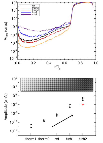
Figure 28: Top: Radial rms velocity as a function of normalized radius for five different models whose characteristics are summarized in Tab 1. Bottom: Amplitude of the most powerful peak in each model. We find that some waves in turb2 have sufficient amplitudes to go through the convective zone and emerge on the surface of the star (top boundary at $0.97R_{\odot}$). The hatched zone represents the values of surface solar g-modes predicted in the literature.

6 Conclusion

In this paper, we have presented the first study of IGWs stochastic excitation and propagation in a 3D spherical Sun using a realistic stratification in the radiative zone and a nonlinear coupling between radiative and convective zones. This configuration allows a direct comparison with seismic studies. These results are extremely rich, and we stand yet at the beginning of their exploration and comprehension.

Since Brun & Zahn (2006), the ASH code has entered a new area because it is no longer dedicated to the study of convective envelopes alone (Elliott et al., 2000; Brun & Toomre, 2002). The nonlinear coupling with the inner radiative zone opens up a large field of investigation. We presented two recent improvements in the ASH code that have a strong impact on our study of gravity waves.

• On one hand, the implementation of the LBR equations (Brown et al., 2012) ensures the right conservation of energy in the radiative zone and allows IGWs’ frequencies and amplitudes to be computec with a better accuracy.

• On the other hand, the extension of the computational domain to $r=0$ by imposing special boundary conditions (Bayliss et al., 2007) largely improves the treatment of g-modes since we now model the entire radiative cavity without any central cutoff (Brun et al., 2011; Alvan et al., 2012).

We then discussed the convective overshoot observed in our models and related this process to the excitation of a large spectrum of IGWs, in agreement with both fluid mechanics and stellar oscillations theory predictions. This spectrum extends from zero to the maximum of the BV frequency ($\sim$0.45mHz), which implies that both propagative (low-frequency) and standing waves (high-frequency) must be represented. Using our raytracing code (e.g., Gough, 1993; Christensen-Dalsgaard, 1997) also contributes to improving our understanding and illustrates the behavior of IGWs as propagative waves, their group and phase velocity, and their location in the 3D sphere. This underlines the complementarity between our simulations of the Sun and linear and asymptotic theories and models.

The properties of the spectrum of IGWs presented in this paper are multiple. To understand its structure, we decomposed it into its spatial and temporal parts, and retrieved the results of Belkacem et al. (2009) predicting that the frequency spectrum was better fitted with a Lorentzian-like function rather than with a Gaussian function. We also showed the quick drop of energy with increasing wavenumbers $k_{h}$. Then, we presented the changes in this spectrum as a function of the depth and proposed a distinction between propagative waves and g-modes. Indeed, this subject is rather hazy in the literature, and it is sometimes difficult to place the limit between both types. Although they correspond to the same physical process, only g-mode frequencies are described by integers $n$. We then discussed some important properties relative to g-modes.

• We applied the same method as Garcia et al. (2007) to detect g-modes signatures at the surface of the Sun and confirmed that the stratification chosen in the model plays an important role in the calculation of g-modes frequencies.

• We also had a look at the impact of the rotation on g-modes, whose frequencies were splitted with respect to their azimuthal number $m$. We showed that the precision of the inversion process strongly depends on the radial order of the modes that are considered and that one must take at least up to $n$=25 to get a precision of 5% in the estimation of the rotation rate.

• Finally, we explained that the energy is not equally distributed into values of $m$ but is instead distributed in high $m$. That shows that the assumption made in several codes, supposing an equal distribution of the energy must be treated with caution. Moreover, since high $m$ modes are located close to the equator, these results could orient the research of g-modes at the surface of the Sun. This last result, in particular, could not have been obtained without taking the three dimensions of the problem into account.

Finally, we dealt with the energy transferred from the convection to IGWS and then carried by them.

• We showed that the different formula supplied by the literature to estimate this energy give a comparable estimation of the percentage of the solar luminosity carried by waves. Indeed, we found that about 0.4% of the solar luminosity is converted into waves at the interface between radiative and convective zones.

• We pointed out that the radiative damping predicted by the linear theory is much stronger than the one observed and partly explained this difference by considering the impact of the nonlinear processes.

• Concerning, finally, the amplitude of g-modes that could be detected at the surface of the Sun, we are not yet able to reach the required domain of parameters but we showed a promising trend toward a good estimation of these amplitudes.

Our results are of interest for several astrophysical applications. The part concerning g-modes is directly related to helioseimology. The asteroseismology community can be concerned by a better understanding of the waves and also seeing that other types of stars can be simulated by the ASH code. Concerning low-frequency propagating IGWs, our work provides new information about the radiative damping and the related effect of nonlinearities to be considered. The spectra presented and the radiative damping found can be implemented in stellar evolution codes to provide a more realistic repartition of energy, especially concerning the distribution accross $m$ components.

Finally, some perspectives of this work are identifiable and will be the object of future works. We presented in Sect. 4.3.2 our first results concerning the effect of the rotation on IGWs. Following Dintrans & Rieutord (2000), Ballot et al. (2010), and Rogers et al. (2013), it could be possible to study the behavior of IGWs in rapidly rotating stars (Mathis & Neiner, 2013) and the transport of angular momentum by gravito-inertial waves (Mathis et al., 2008; Mathis, 2009). Also of great interest could be the addition of a magnetic field in the simulations to characterize its impact on IGWs (Goode & Thompson, 1992; Rogers & MacGregor, 2010; Mathis & de Brye, 2011, 2012). Indeed, the presence of a magnetic field will modify the dispersion relation. If its amplitude is high enough, we can anticipate that a large-scale magnetic field trapped in the radiative zone will have a significant impact on the propagation of IGWs, such as wave reflexions, filtering, and frequency shift. Particularly, for waves frequencies close to the Alfven frequency, IGWs will be trapped vertically, while for frequencies below the inertial frequency ($2\Omega$) some equatorial trapping will occur. Moreover, we could expect that a time-dependent magnetic field generated by dynamo action would modulate the waves’ signal.

This work thus constitutes a first cornerstone where the completementary use of 3D nonlinear simulations and of asymptotic theories allows bringing the study of the excitation, propagation, and damping of gravity waves in stellar interiors to a new level of understanding. Morever, the potential application to other types of rotating and possibly magnetic stars open a new window in theoretical asteroseismology in the whole HR diagram.

Appendix A: Inner boundary conditions

The authors are keen to thank N. Featherstone for the time spent with A.S. Brun to develop and test the full sphere version of ASH (as explained in this appendix), which allowed a more precise analysis of the gravity wave’s properties in the whole radiative interior. We here follow the method proposed by Bayliss (2006) to obtain the inner boundary conditions for ${Z}$ and ${W}$. For the sake of clarity in the following equations, we introduce the notation $\@vec{X}=\@vec{\bar{\rho}\@vec{\mathrm{v}}}$ and do not write the subscripts $\ell,m$ if there is another subscript.

Starting from the poloidal-toroidal decomposition of $\@vec{X}=\@vec{\bar{\rho}\@vec{\mathrm{v}}}$ (Eq. (8)), we project ${Z}$ and ${W}$ on the spherical harmonics basis

$$\left\{\begin{array}[]{ll}{Z}(r,\theta,\varphi)&=\displaystyle\sum_{\ell m}{Z}_{\ell m}(r)\mathrm{Y}_{\ell m}(\theta,\varphi)\hbox{,}\\ {W}(r,\theta,\varphi)&=\displaystyle\sum_{\ell m}{W}_{\ell m}(r)\mathrm{Y}_{\ell m}(\theta,\varphi)\hbox{,}\end{array}\right.$$ (42)

which leads to

$$\@vec{X} = \sum_{\ell m}\left(\underbrace{\frac{l(l+1)}{r^{2}}{W}_{\ell m}\mathrm{Y}_{\ell m}}_{{{X_{{W}r}}}}\right)\@vec{e}_{r}$$

$$+ \sum_{\ell m}\left(\underbrace{\frac{1}{r}\partial_{r}({W}_{\ell m})\partial_{\theta}(\mathrm{Y}_{\ell m})}_{{{X_{{W}\theta}}}}+\underbrace{\frac{1}{r\sin\theta}{Z}_{\ell m}\partial_{\varphi}(\mathrm{Y}_{\ell m})}_{{{X_{{Z}\theta}}}}\right)\@vec{e}_{\theta}$$

$$+ \sum_{\ell m}\left(\underbrace{\frac{1}{r\sin\theta}\partial_{r}({W}_{\ell m})\partial_{\varphi}(\mathrm{Y}_{\ell m})}_{{{X_{{W}\varphi}}}}-\underbrace{\frac{1}{r}{Z}_{\ell m}\partial_{\theta}(\mathrm{Y}_{\ell m})}_{{{-X_{{Z}\varphi}}}}\right)\@vec{e}_{\varphi}\hbox{.}$$

We then expand ${Z}$ and ${W}$ in Taylor series in the vicinity of $r=0$

$$\left\{\begin{array}[]{ll}{W}_{\ell m}(r)&={W}_{0}+r{W}^{\prime}_{0}+\displaystyle\frac{r^{2}}{2!}{W}^{\prime\prime}_{0}+\displaystyle\frac{r^{3}}{3!}{W}^{(3)}_{0}+\displaystyle\frac{r^{4}}{4!}{W}^{(4)}_{0}\hbox{,}\\ {Z}_{\ell m}(r)&={Z}_{0}+r{Z}^{\prime}_{0}+\displaystyle\frac{r^{2}}{2!}{Z}^{\prime\prime}_{0}+\displaystyle\frac{r^{3}}{3!}{Z}^{(3)}_{0}+\displaystyle\frac{r^{4}}{4!}{Z}^{(4)}_{0}\hbox{,}\end{array}\right.$$ (44)

where ${W}_{0}\equiv{W}_{\ell m}\lvert_{r=0}$, ${W}^{\prime}_{0}\equiv\displaystyle\frac{\partial{W}_{\ell m}}{\partial r}\biggr{\lvert}_{r=0}$, ${W}^{\prime\prime}_{0}\equiv\displaystyle\frac{\partial^{2}{W}_{\ell m}}{\partial r^{2}}\biggr{\lvert}_{r=0}$…

Replacing these developments in Eq. (Appendix A: Inner boundary conditions), we obtain the expression of $\@vec{X}$ as a function of the derivatives of ${W}_{\ell m}$ and ${Z}_{\ell m}$ at $r=0$.

The central boundary conditions come from the fact that no cartesian component can depend on the angles $\theta$ and $\varphi$. In this case, the vector $\@vec{X}$ would be multi valued at the origin. Thus, we write the cartesian components of $\@vec{X}$ as a function of its spherical components

$$\left\{\begin{array}[]{ll}{X}_{x}&=X_{r}\sin\theta\cos\varphi+X_{\theta}\cos\theta\cos\varphi-X_{\varphi}\sin\varphi\hbox{,}\\ {X}_{y}&=X_{r}\sin\theta\sin\varphi+X_{\theta}\cos\theta\sin\varphi+X_{\varphi}\cos\varphi\hbox{,}\\ {X}_{z}&=X_{r}\cos\theta-X_{\theta}\sin\theta\hbox{,}\end{array}\right.$$ (45)

where $X_{r}=X_{{W}r}$, ${{X_{\theta}}}={{X_{{W}\theta}}}+{{X_{{Z}\theta}}}$ and $X_{\varphi}={{X_{{W}\varphi}}}+{{X_{{Z}\varphi}}}$, and then rewrite ${X}_{x}$, ${X}_{y}$, and ${X}_{z}$ by replacing ${W}_{\ell m}$ and ${Z}_{\ell m}$ with their Taylor developments. Terms of first order and above in $r$ will be zero as $r\to 0$, but other terms that depend on $\theta$ and $\varphi$ must be set to zero by the choice of the values of ${W}_{0}$, ${W}^{\prime}_{0}$, ${W}^{\prime\prime}_{0}$, ${Z}_{0}$, ${Z}^{\prime}_{0}$, and ${Z}^{\prime\prime}_{0}$.

For $\ell=1$ and $m=0$, we obtain

$$X_{x}(r,\theta,\varphi)\biggr{\lvert}_{1,0} = -\frac{1}{2}\sqrt{\frac{3}{\pi}}\sin\theta\sin\varphi{Z}^{\prime}_{0}$$

$$-\sqrt{\frac{3}{\pi}}\frac{\sin\theta}{2r}\left(-\cos\theta\cos\varphi{W}^{\prime}_{0}+\sin\varphi{Z}_{0}\right)$$

$$+\sqrt{\frac{3}{\pi}}\frac{1}{r^{2}}\cos\theta\sin\theta\cos\varphi{W}_{0}$$

$$-\frac{r\sin\theta}{4\sqrt{3\pi}}\left(\cos\theta\cos\varphi{W}^{(3)}_{0}+3\sin\varphi{Z}^{\prime\prime}_{0}\right)$$

$$-\frac{r^{2}\sin\theta}{8\sqrt{3\pi}}\left(\cos\theta\cos\varphi{W}^{(4)}_{0}+2\sin\varphi{Z}^{(3)}_{0}\right)$$

$$-\frac{r^{3}}{16\sqrt{3\pi}}\sin\theta\sin\varphi{Z}^{(4)}_{0}\hbox{.}$$

• The first term on the righthand side is constant with respect to $r$, but since $X_{x}$ cannot depend on $\theta$ and $\varphi$, we must impose ${Z}^{\prime}_{0}=0$.

• The two following terms diverge when $r\to 0$, so we must impose ${W}^{\prime}_{0}={Z}_{0}=0$ and ${W}_{0}=0$.

• The remaining terms tend to 0 with $r$.

Then,

$$X_{y}(r,\theta,\varphi)\biggr{\lvert}_{1,0} = \frac{1}{2}\sqrt{\frac{3}{\pi}}\sin\theta\cos\varphi{Z}^{\prime}_{0}$$

$$+\sqrt{\frac{3}{\pi}}\frac{\sin\theta}{2r}\left(\cos\varphi{Z}_{0}+\cos\theta\sin\varphi{W}^{\prime}_{0}\right)$$

$$+\sqrt{\frac{3}{\pi}}\frac{1}{r^{2}}\cos\theta\sin\theta\sin\varphi{W}_{0}$$

$$+\frac{r\sin\theta}{4\sqrt{3\pi}}\left(3\cos\varphi{Z}^{(2)}_{0}-\cos\theta\sin\varphi{W}^{(3)}_{0}\right)$$

$$+\frac{r^{2}\sin\theta}{8\sqrt{3\pi}}\left(2\cos\varphi{Z}^{(3)}_{0}-\cos\theta\sin\varphi{W}^{(4)}_{0}\right)$$

$$+\frac{r^{3}}{16\sqrt{3\pi}}\sin\theta\cos\varphi{Z}^{(4)}_{0}\hbox{.}$$

The conditions to impose are ${Z}^{\prime}_{0}=0$ for the constant term, ${Z}_{0}={W}^{\prime}_{0}=0$ for the term varying in $1/r$ and ${W}_{0}=0$ for the one varying in $1/r^{2}$. Finally,

$$X_{z}(r,\theta,\varphi)\biggr{\lvert}_{1,0} = \frac{1}{2}\sqrt{\frac{3}{\pi}}{W}^{\prime\prime}_{0}$$

$$+\sqrt{\frac{3}{\pi}}\frac{1}{4r}\left(3+\cos 2\theta\right){W}^{\prime}_{0}$$

$$+\sqrt{\frac{3}{\pi}}\frac{1}{2r^{2}}\left(1+\cos 2\theta\right){W}_{0}$$

$$+\frac{r}{8\sqrt{3\pi}}\left(5-\cos 2\theta\right){W}^{(3)}_{0}$$

$$+\frac{r^{2}}{16\sqrt{3\pi}}\left(3-\cos 2\theta\right){W}^{(4)}_{0}\hbox{.}$$

This time, the constant term does not vary with $\theta$ or $\varphi$, so there is no need to nullify it. The divergent terms impose the conditions ${W}_{0}=0$ and ${W}^{\prime}_{0}=0$.
We obtain the conditions for $\ell\neq 1$ by applying the same calculation to, for example, $\ell=2$ and $m=0$:

$$X_{x}(r,\theta,\varphi)\biggr{\lvert}_{2,0} = -\frac{3\sin\theta}{4}\sqrt{\frac{5}{\pi}}\left(\sin^{2}\theta\cos\varphi{W}^{\prime\prime}_{0}+2\cos\theta\sin\varphi{Z}^{\prime}_{0}\right)$$

$$-\frac{3\sin\theta}{2r}\sqrt{\frac{5}{\pi}}\left(-\cos 2\theta\cos\varphi{W}^{\prime}_{0}+\cos\theta\sin\varphi{Z}_{0}\right)$$

$$-\frac{3}{2r^{2}}\sqrt{\frac{5}{\pi}}\sin\theta\cos\varphi{W}_{0}\left(1-3\cos^{2}\theta\right)$$

$$-\frac{r\sin\theta}{4}\sqrt{\frac{5}{\pi}}\left(\cos\varphi{W}^{(3)}_{0}+3\cos\theta\sin\varphi{Z}^{\prime\prime}_{0}\right)$$

$$-\frac{r^{2}\sin\theta}{16}\sqrt{\frac{5}{\pi}}\left((1+\cos^{2}\theta)\cos\varphi{W}^{(4)}_{0}\right.$$

$$\hbox{\hskip 113.81102pt}+\left.4\cos\theta\sin\varphi{Z}^{(3)}_{0}\right)$$

$$-\frac{r^{3}}{16}\sqrt{\frac{5}{\pi}}\cos\theta\sin\theta\sin\varphi{Z}^{(4)}_{0}\hbox{,}$$

$$X_{y}(r,\theta,\varphi)\biggr{\lvert}_{2,0} = \frac{3\sin\theta}{4}\sqrt{\frac{5}{\pi}}\left(2\cos\theta\cos\varphi{Z}^{\prime}_{0}+\sin^{2}\theta\sin\varphi{W}^{\prime\prime}_{0}\right)$$

$$+\frac{3\sin\theta}{2r}\sqrt{\frac{5}{\pi}}\left(-\sin^{2}\theta\sin\varphi{W}^{\prime}_{0}+\cos\theta\cos\varphi{Z}_{0}\right)$$

$$-\frac{3\sin\theta}{2r^{2}}\sqrt{\frac{5}{\pi}}\left(1-3\cos^{2}\theta\right)\sin\varphi{W}_{0}$$

$$+\frac{r\sin\theta}{4}\sqrt{\frac{5}{\pi}}\left(3\cos\theta\cos\varphi{Z}^{\prime\prime}_{0}-\sin\varphi{W}^{(3)}_{0}\right)$$

$$-\frac{r^{2}\sin\theta}{16}\sqrt{\frac{5}{\pi}}\left((1+\cos^{2}\theta)\sin\varphi{W}^{(4)}_{0}\right.$$

$$\hbox{\hskip 113.81102pt}-\left.4\cos\theta\cos\varphi{Z}^{(3)}_{0}\right)$$

$$+\frac{r^{3}}{16}\sqrt{\frac{5}{\pi}}\cos\theta\sin\theta\cos\varphi{Z}^{(4)}_{0}\hbox{,}$$

and

$$X_{z}(r,\theta,\varphi)\biggr{\lvert}_{2,0} = \frac{3\cos\theta}{8}\sqrt{\frac{5}{\pi}}\left(3+\cos 2\theta\right){W}^{\prime\prime}_{0}$$

$$+\frac{3\cos\theta}{2r}\sqrt{\frac{5}{\pi}}\left(1+\cos 2\theta\right){W}^{\prime}_{0}$$

$$+\frac{3\cos\theta}{4r^{2}}\sqrt{\frac{5}{\pi}}\left(1+3\cos 2\theta\right){W}_{0}$$

$$+\frac{r\cos\theta}{2}\sqrt{\frac{5}{\pi}}{W}^{(3)}_{0}$$

$$+\frac{r^{2}\cos\theta}{32}\sqrt{\frac{5}{\pi}}\left(5-\cos 2\theta\right){W}^{(4)}_{0}\hbox{.}$$

Finally, the conditions to impose at $r=0$ are

• ${Z}_{0}={Z}^{\prime}_{0}=0$ and ${W}_{0}={W}^{\prime}_{0}=0$ for $\ell=1$,

• ${Z}_{0}={Z}^{\prime}_{0}=0$ and ${W}_{0}={W}^{\prime}_{0}={W}^{\prime\prime}_{0}=0$ for $\ell\neq 1$.

Considering the order of the equations verified by $\mathrm{Z_{\ell m}}$ and ${W}_{\ell m}$, we can impose only one condition for $\mathrm{Z_{\ell m}}$ and two for $\mathrm{W_{\ell m}}$ at each limit of the domain. Thus, we have made the choice to distinguish between $\ell=1$ and $\ell\neq 1$ by imposing (set 1):

• ${Z}_{0}=0$ for all $\ell$,

• ${W}_{0}={W}^{\prime}_{0}=0$ for $\ell=1$,

• ${W}_{0}={W}^{\prime\prime}_{0}=0$ for $\ell\neq 1$,

but another possible set is (set 2):

• ${Z}_{0}=0$ for all $\ell$,

• ${W}_{0}={W}^{\prime}_{0}=0$ for all $\ell$.

In Fig. 29, we compare the model ref developed in the current article with another model calculated with set 2 (every other parameter is identical). The radial and horizontal rms velocities in both models differ from less than 0.1%.

For a better numerical stability, a more stringent condition could be to impose $Z,W\to r^{l+1}$ as $r\to 0$ (Bayliss et al., 2007; Livermore et al., 2007; Glatzmaier, 2013).

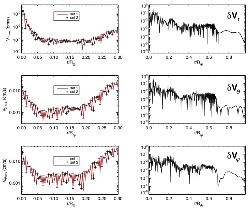
Figure 29: Left: Radial and horizontal rms velocities as a function of the normalized radius for model ref (red line, calculated with set 1) and the same model (black crosses) calculated with set 2 at time t $\approx$ 90 days. Both curves are almost perfectly superimposed. Right: Difference between both models in percent: $\biggr{\lvert}\displaystyle\frac{\mathrm{v}_{1}-\mathrm{v}_{2}}{\mathrm{v}_{1}}\biggr{\rvert}\times 100$, where $\mathrm{v}_{1}$ corresponds to model ref and $\mathrm{v}_{2}$ to the other one. The difference at $r=0$ is about 0.1% and much less in the rest of the sphere.

References

- Aerts et al. (2010) Aerts, C., Christensen-Dalsgaard, J., & Kurtz, D. D. W. 2010, Asteroseismology, Astronomy and Astrophysics Library (Springer London, Limited)
- Alvan et al. (2012) Alvan, L., Brun, A. S., & Mathis, S. 2012, in SF2A-2012: Proceedings of the Annual meeting of the French Society of Astronomy and Astrophysics. Eds.: S. Boissier, 289–293
- Alvan et al. (2013) Alvan, L., Mathis, S., & Decressin, T. 2013, Astronomy and Astrophysics, 553, 86
- Andersen (1994) Andersen, B. N. 1994, Solar Physics (ISSN 0038-0938), 152, 241
- Andersen (1996) Andersen, B. N. 1996, Astronomy and Astrophysics, 312, 610
- Andreassen et al. (1992) Andreassen, O., Andersen, B. N., & Wasberg, C. E. 1992, Astronomy and Astrophysics (ISSN 0004-6361), 257, 763
- Appourchaux et al. (2010) Appourchaux, T., Belkacem, K., Broomhall, A.-M., et al. 2010, A&A Rev., 18, 197
- Baldwin et al. (2001) Baldwin, M. P., Gray, L. J., Dunkerton, T. J., et al. 2001, Reviews of Geophysics, 39, 179
- Ballot et al. (2010) Ballot, J., Lignières, F., Reese, D. R., & Rieutord, M. 2010, A&A, 518, A30
- Bayliss (2006) Bayliss, R. A. 2006, PhD thesis, University of Wisconsin-Madison
- Bayliss et al. (2007) Bayliss, R. A., Forest, C. B., Nornberg, M. D., Spence, E. J., & Terry, P. W. 2007, Physical Review E, 75, 26303
- Beck et al. (2012) Beck, P. G., Montalban, J., Kallinger, T., et al. 2012, Nature, 481, 55
- Bedding et al. (2011) Bedding, T. R., Mosser, B., Huber, D., et al. 2011, Nature, 471, 608
- Belkacem et al. (2009) Belkacem, K., Mathis, S., Goupil, M. J., & Samadi, R. 2009, Astronomy and Astrophysics, 508, 345
- Belkacem et al. (2009) Belkacem, K., Mathis, S., Goupil, M. J., & Samadi, R. 2009, A&A, 508, 345
- Belkacem et al. (2009) Belkacem, K., Samadi, R., Goupil, M. J., et al. 2009, Astronomy and Astrophysics, 494, 191
- Berthomieu & Provost (1990) Berthomieu, G. & Provost, J. 1990, Astronomy and Astrophysics (ISSN 0004-6361), 227, 563
- Berthomieu & Provost (1991) Berthomieu, G. & Provost, J. 1991, IRIS /International Research on the Interior of the Sun/ Workshop, 133, 127
- Booker & Bretherton (1967) Booker, J. & Bretherton, F. 1967, Journal of Fluid Mechanics, 27, 513
- Braginsky & Roberts (1995) Braginsky, S. I. & Roberts, P. H. 1995, Geophysical and Astrophysical Fluid Dynamics, 79, 1
- Brown et al. (2012) Brown, B. P., Vasil, G. M., & Zweibel, E. G. 2012, ApJ, 756, 109
- Browning et al. (2004) Browning, M., Brun, A. S., & Toomre, J. 2004, ApJ, 601, 512
- Brun et al. (2002) Brun, A. S., Antia, H. M., Chitre, S. M., & Zahn, J.-P. 2002, Astronomy and Astrophysics, 391, 725
- Brun et al. (2004) Brun, A. S., Miesch, M. S., & Toomre, J. 2004, ApJ, 614, 1073
- Brun et al. (2011) Brun, A. S., Miesch, M. S., & Toomre, J. 2011, ApJ, 742, 79
- Brun & Toomre (2002) Brun, A. S. & Toomre, J. 2002, ApJ, 570, 865
- Brun et al. (1998) Brun, A. S., Turck-Chièze, S., & Morel, P. 1998, ApJ, 506, 913
- Brun & Zahn (2006) Brun, A. S. & Zahn, J.-P. 2006, Astronomy and Astrophysics, 457, 665
- Chanmugam (1972) Chanmugam, G. 1972, Nature Physical Science, 236, 83
- Charbonnel et al. (2013) Charbonnel, C., Decressin, T., Amard, L., Palacios, A., & Talon, S. 2013, Astronomy and Astrophysics, 554, A40
- Charbonnel & Talon (2005) Charbonnel, C. & Talon, S. 2005, Science, 309, 2189
- Christensen-Dalsgaard (1997) Christensen-Dalsgaard, J. 1997, Lecture Notes on Stellar Oscillations
- Christensen-Dalsgaard et al. (1995) Christensen-Dalsgaard, J., Bedding, T. R., & Kjeldsen, H. 1995, Astrophysical Journal, 443, L29
- Clune et al. (1999) Clune, T., Elliott, J., Miesch, M. S., Toomre, J., & Glatzmaier, G. A. 1999, Parallel Computing, 25, 361
- De Cat et al. (2011) De Cat, P., Uytterhoeven, K., Gutiérrez-Soto, J., Degroote, P., & Simón-Díaz, S. 2011, Stellar Instability and Evolution, 6, 433
- Deheuvels et al. (2012) Deheuvels, S., Garcia, R., Chaplin, W. J., et al. 2012, The astrophysical journal, 756, 19
- Dintrans et al. (2005) Dintrans, B., Brandenburg, A., Nordlund, Å., & Stein, R. F. 2005, Astronomy and Astrophysics, 438, 365
- Dintrans & Rieutord (2000) Dintrans, B. & Rieutord, M. 2000, Astronomy and Astrophysics, 354, 86
- Domingo et al. (1995) Domingo, V., Fleck, B., & Poland, A. I. 1995, Space Science Reviews, 72, 81
- Duez & Mathis (2010) Duez, V. & Mathis, S. 2010, Astronomy and Astrophysics, 517, A58
- Dunkerton (1997) Dunkerton, T. J. 1997, Journal of Geophysical Research, 102, 26053
- Elliott et al. (2000) Elliott, J., Miesch, M. S., & Toomre, J. 2000, The astrophysical journal, 533, 546
- Fritts et al. (1998) Fritts, D. C., Vadas, S. L., & Andreassen, O. 1998, Astronomy and Astrophysics, 333, 343
- Garaud & Garaud (2008) Garaud, P. & Garaud, J. D. 2008, Monthly Notices of the Royal Astronomical Society, 391, 1239
- Garcia et al. (2007) Garcia, R. A., Turck-Chièze, S., Jiménez-Reyes, S. J., et al. 2007, Science, 316, 1591
- Garcia Lopez & Spruit (1991) Garcia Lopez, R. J. & Spruit, H. C. 1991, Astrophysical Journal, 377, 268
- Gastine & Dintrans (2010) Gastine, T. & Dintrans, B. 2010, Astrophysics and Space Science, 328, 245
- Giorgetta et al. (2002) Giorgetta, M. A., Manzini, E., & Roeckner, E. 2002, Geophysical Research Letters, 29, 1245
- Glatzmaier (1984) Glatzmaier, G. A. 1984, Journal of Computational Physics (ISSN 0021-9991), 55, 461
- Glatzmaier (2013) Glatzmaier, G. A. 2013, Introduction to Modeling Convection in Planets and Stars : Magnetic Filed, Density stratification, Rotation (Princeton University Press)
- Goldreich & Kumar (1990) Goldreich, P. & Kumar, P. 1990, Astrophysical Journal, 363, 694
- Goldreich et al. (1994) Goldreich, P., Murray, N., & Kumar, P. 1994, Astrophysical Journal, 424, 466
- Goode & Thompson (1992) Goode, P. R. & Thompson, M. J. 1992, ApJ, 395, 307
- Gough (1986) Gough, D. 1986, Seismology of the Sun and the Distant Stars, C: Nato advanced science institutes series (D. Reidel Publishing Company)
- Gough (1993) Gough, D. 1993, In: Astrophysical Fluid Dynamics - Les Houches 1987, 399–560
- Gough & McIntyre (1998) Gough, D. & McIntyre, M. 1998, Nature, 394, 755
- Green et al. (2003) Green, E. M., Fontaine, G., Reed, M. D., et al. 2003, ApJ, 583, L31
- Hurlburt et al. (1986) Hurlburt, N. E., Toomre, J., & Massaguer, J. M. 1986, Astrophysical Journal, 311, 563
- Hurlburt et al. (1994) Hurlburt, N. E., Toomre, J., Massaguer, J. M., & Zahn, J.-P. 1994, Astrophysical Journal, 421, 245
- Jones et al. (2011) Jones, C. A., Boronski, P., Brun, A. S., et al. 2011, Icarus, 216, 120
- Kiraga et al. (2003) Kiraga, M., Jahn, K., Stepien, K., & Zahn, J.-P. 2003, Acta Astronomica, 53, 321
- Kiraga et al. (2005) Kiraga, M., Stepien, K., & Jahn, K. 2005, Acta Astronomica, 55, 205
- Kumar & Quataert (1995) Kumar, P. & Quataert, E. 1995, 1
- Kumar et al. (1999) Kumar, P., Talon, S., & Zahn, J.-P. 1999, ApJ, 520, 859
- Landolt (1968) Landolt, A. U. 1968, Astrophysical Journal, 153, 151
- Lantz (1992) Lantz, S. R. 1992, PhD thesis, Cornell University
- Lecoanet & Quataert (2013) Lecoanet, D. & Quataert, E. 2013, MNRAS, 430, 2363
- Lighthill (1978) Lighthill, J. 1978, Cambridge
- Lighthill (1986) Lighthill, J. 1986, Provided by the SAO/NASA Astrophysics Data System
- Livermore et al. (2007) Livermore, P. W., Jones, C. A., & Worland, S. J. 2007, Journal of Computational Physics, 227, 1209
- Massaguer et al. (1984) Massaguer, J. M., Latour, J., Toomre, J., & Zahn, J.-P. 1984, Astronomy and Astrophysics (ISSN 0004-6361), 140, 1
- Mathis (2009) Mathis, S. 2009, Astronomy and Astrophysics, 506, 811
- Mathis & de Brye (2011) Mathis, S. & de Brye, N. 2011, Astronomy and Astrophysics, 526, A65
- Mathis & de Brye (2012) Mathis, S. & de Brye, N. 2012, Astronomy and Astrophysics, 1
- Mathis et al. (2013) Mathis, S., Decressin, T., Eggenberger, P., & Charbonnel, C. 2013, Astronomy and Astrophysics, 558, 11
- Mathis & Neiner (2013) Mathis, S. & Neiner, C. 2013, SF2A-2013: Proceedings of the Annual meeting of the French Society of Astronomy and Astrophysics, -1, 241
- Mathis et al. (2008) Mathis, S., Talon, S., Pantillon, F. P., & Zahn, J.-P. 2008, Solar Physics, 251, 101
- Mathis & Zahn (2004) Mathis, S. & Zahn, J.-P. 2004, A&A, 425, 229
- Mathur et al. (2008) Mathur, S., Eff-Darwich, A., García, R. A., & Turck-Chièze, S. 2008, A&A, 484, 517
- Miesch et al. (2000) Miesch, M. S., Elliott, J. R., Toomre, J., et al. 2000, The astrophysical journal, 532, 593
- Montalban, J. (1994) Montalban, J. 1994, Astronomy and Astrophysics, 281, 421
- Moravveji et al. (2012) Moravveji, E., Moya, A., & Guinan, E. F. 2012, ApJ, 749, 74
- Mosser et al. (2013) Mosser, B., Belkacem, K., & Vrard, M. 2013, astro-ph
- Mosser et al. (2013) Mosser, B., Samadi, R., & Belkacem, K. 2013, 25
- Müller et al. (1986) Müller, P., Holloway, G., Henyey, F., & Pomphrey, N. 1986, Reviews of Geophysics, 24, 493
- Neiner et al. (2012) Neiner, C., Floquet, M., Samadi, R., et al. 2012, Astronomy and Astrophysics, 546, 47
- Plumb & McEwan (1978) Plumb, R. A. & McEwan, A. D. 1978, Journal of Atmospheric Sciences, 35, 1827
- Press (1981) Press, W. H. 1981, ApJ, 245, 286
- Provost & Berthomieu (1986) Provost, J. & Berthomieu, G. 1986, Astronomy and Astrophysics (ISSN 0004-6361), 165, 218
- Rogers & Glatzmaier (2005a) Rogers, T. M. & Glatzmaier, G. A. 2005a, Monthly Notices of the Royal Astronomical Society, 364, 1135
- Rogers & Glatzmaier (2005b) Rogers, T. M. & Glatzmaier, G. A. 2005b, The astrophysical journal, 620, 432
- Rogers & Glatzmaier (2006) Rogers, T. M. & Glatzmaier, G. A. 2006, The astrophysical journal, 653, 756
- Rogers et al. (2006) Rogers, T. M., Glatzmaier, G. A., & Jones, C. A. 2006, ApJ, 653, 765
- Rogers et al. (2013) Rogers, T. M., Lin, D. N. C., McElwaine, J. N., & Lau, H. H. B. 2013, ApJ, 772, 21
- Rogers & MacGregor (2010) Rogers, T. M. & MacGregor, K. B. 2010, Monthly Notices of the Royal Astronomical Society, 401, 191
- Rogers et al. (2008) Rogers, T. M., MacGregor, K. B., & Glatzmaier, G. A. 2008, MNRAS, 387, 616
- Saikia et al. (2000) Saikia, E., Singh, H. P., Chan, K. L., Roxburgh, I. W., & Srivastava, M. P. 2000, The astrophysical journal, 529, 402
- Samadi et al. (2003) Samadi, R., Nordlund, Å., Stein, R. F., Goupil, M. J., & Roxburgh, I. 2003, A&A, 403, 303
- Schatzman (1993) Schatzman, E. 1993, Astronomy and Astrophysics (ISSN 0004-6361), 279, 431
- Schatzman (1996) Schatzman, E. 1996, Solar Physics, 169, 245
- Shiode et al. (2013) Shiode, J. H., Quataert, E., Cantiello, M., & Bildsten, L. 2013, Monthly Notices of the Royal Astronomical Society, 430, 1736
- Spiegel & Zahn (1992) Spiegel, E. & Zahn, J.-P. 1992, Astronomy and Astrophysics, 265, 106
- Strugarek et al. (2011a) Strugarek, A., Brun, A. S., & Zahn, J.-P. 2011a, astro-ph, 34
- Strugarek et al. (2011b) Strugarek, A., Brun, A. S., & Zahn, J.-P. 2011b, Astronomische Nachrichten, 332, 891
- Talon & Charbonnel (2003) Talon, S. & Charbonnel, C. 2003, A&A, 405, 1025
- Talon & Charbonnel (2005) Talon, S. & Charbonnel, C. 2005, Astronomy and Astrophysics, 440, 981
- Talon & Charbonnel (2008) Talon, S. & Charbonnel, C. 2008, A&A, 482, 597
- Thompson et al. (2003) Thompson, M. J., Christensen-Dalsgaard, J., Miesch, M. S., & Toomre, J. 2003, Annual Review of Astronomy &Astrophysics, 41, 599
- Turck-Chièze et al. (2004) Turck-Chièze, S., Garcia, R., Couvidat, S., et al. 2004, The astrophysical journal, 604, 455
- Unno et al. (1989) Unno, W., Osaki, Y., Ando, H., Saio, H., & Shibahashi, H. 1989, Nonradial oscillations of stars
- Vauclair (2005) Vauclair, G. 2005, EAS Publications Series, 17, 133
- Voisin (1991) Voisin, B. 1991, Journal of Fluid Mechanics, 231, 439
- Waelkens (1991) Waelkens, C. 1991, Astronomy and Astrophysics (ISSN 0004-6361), 246, 453
- Warner & Robinson (1972) Warner, B. & Robinson, E. L. 1972, Nature Physical Science, 239, 2
- Winget & Kepler (2008) Winget, D. E. & Kepler, S. O. 2008, ARA&A, 46, 157
- Zahn (1983) Zahn, J.-P. 1983, Saas-Fee Advanced Course 13, 253
- Zahn (1991) Zahn, J.-P. 1991, Astronomy and Astrophysics (ISSN 0004-6361), 252, 179
- Zahn (1992) Zahn, J.-P. 1992, Astronomy and Astrophysics (ISSN 0004-6361), 265, 115
- Zahn et al. (1997) Zahn, J.-P., Talon, S., & Matias, J. 1997, Astronomy and Astrophysics, 322, 320