A graph/particle-based method for experiment design in nonlinear systems

Abstract

We propose an extended method for experiment design in nonlinear state space models. The proposed input design technique optimizes a scalar cost function of the information matrix, by computing the optimal stationary probability mass function (pmf) from which an input sequence is sampled. The feasible set of the stationary pmf is a polytope, allowing it to be expressed as a convex combination of its extreme points. The extreme points in the feasible set of pmf’s can be computed using graph theory. Therefore, the final information matrix can be approximated as a convex combination of the information matrices associated with each extreme point. For nonlinear systems, the information matrices for each extreme point can be computed by using particle methods. Numerical examples show that the proposed technique can be successfully employed for experiment design in nonlinear systems.

1 Introduction

Experiment design deals with the generation of an input signal that maximizes the information retrieved from an experiment. Some of the initial contributions are discussed in Cox (1958) and Goodwin and Payne (1977). Since then, many contributions to the subject have been developed; see e.g. Fedorov (1972), Whittle (1973), Hildebrand and Gevers (2003), Gevers (2005) and the references therein.

In this article, a new method for experiment design in nonlinear systems is presented, which extends the input design methods proposed in Gopaluni et al. (2011) and Valenzuela et al. (2013). The objective is to design an experiment as a realization of a stationary process, such that the system is identified with maximum accuracy as defined by a scalar function of the Fisher information matrix, and under the assumption that the input can adopt a finite set of values. The assumption on the input class modifies the class of input sequences considered in Gopaluni et al. (2011). The optimization of the stationary probability mass function (pmf) is done by maximizing a scalar cost function of the information matrix over the feasible set of pmf’s. Using concepts from graph theory (Zaman, 1983; Johnson, 1975; Tarjan, 1972), we can express the feasible set of pmf’s as a convex combination of the measures for the extreme points of the set. Therefore, the information matrix corresponding to a feasible pmf can be expressed as the convex combination of the information matrices associated with the extreme points of the feasible set. Since the exact computation of the information matrices for nonlinear systems is often intractable, we use particle methods to compute sampled information matrices for the extreme points of the feasible set. This allows us to extend the technique of Valenzuela et al. (2013) to more general nonlinear model structures. An attractive property of the method is that the optimization problem is convex even for nonlinear systems. In addition, since the input is restricted to a finite set of possible values, the method can naturally handle amplitude limitations.

Previous results on input design have mostly been concerned with linear systems. A Markov chain approach to input design is presented in Brighenti et al. (2009), where the input is modelled as the output of a Markov chain. Suzuki and Sugie (2007) presents a time domain experiment design method for system identification. Linear matrix inequalities (LMI) are used to solve the input design problem in Jansson and Hjalmarsson (2005) and Lindqvist and Hjalmarsson (2000). A robust approach for input design is presented in Rojas et al. (2007), where the input signal is designed to optimize a cost function over a set where the true parameter is assumed to lie.

In recent years, the interest in input design for nonlinear systems has increased. The main problem here is that the frequency domain approach for experiment design used in linear systems is no longer valid. An analysis of input design for nonlinear systems using the knowledge of linear systems is considered in Hjalmarsson and Mårtensson (2007). In Larsson et al. (2010) an input design method for a particular class of nonlinear systems is presented. Input design for structured nonlinear systems is discussed in Vincent et al. (2009). Gopaluni et al. (2011) introduces a particle filter method for input design in nonlinear systems. An analysis of input design for a class of Wiener systems is considered in Cock et al. (2013). A graph theory approach for input design for output-error like nonlinear system is presented in Valenzuela et al. (2013). The results presented allow to design input signals when the system contains nonlinear functions, but the restrictions on the system dynamics and/or the input structure are the main limitations of most of the previous contributions. Moreover, with the exception of Brighenti et al. (2009), Larsson et al. (2010) and Valenzuela et al. (2013), the proposed methods cannot handle amplitude limitations on the input signal, which could arise due to physical and/or safety reasons.

2 Problem formulation

In this article, the objective is to design an input signal $u_{1:n_{\operatorname{seq}}}:=\{u_{t}\}_{t=1}^{n_{\operatorname{seq}}}$, as a realization of a stationary process. This is done such that a state space model (SSM) can be identified with maximum accuracy as defined by a scalar function of the Fisher information matrix ${\mathcal{I}}_{F}$ (Ljung, 1999). An SSM with states $x_{1:T}:=\{x_{t}\}_{t=1}^{T}$, inputs $u_{1:T}$ and measurements $y_{1:T}$ is given by

$$x_{t}|x_{t-1} \sim f_{\theta}(x_{t}|x_{t-1},u_{t-1}),$$ (1a)

$$y_{t}|x_{t} \sim g_{\theta}(y_{t}|x_{t},u_{t}).$$ (1b)

Here, $f_{\theta}(\cdot)$ and $g_{\theta}(\cdot)$ denote known probability distributions parametrised by $\theta\in\Theta\subset{\mathbb{R}}^{d}$. For the remainder of this article, we make the rather restrictive albeit standard assumption that we know the initial state $x_{0}$ and the true model structure (1) with true parameters $\theta_{0}$. Hence, we can write the joint distribution of states and measurements for (1) as

$$p_{\theta}(x_{1:T},y_{1:T}|u_{1:T})=\prod_{t=1}^{T}f_{\theta}(x_{t}|x_{t-1},u_{t-1})g_{\theta}(y_{t}|x_{t},u_{t}).$$ (2)

This quantity is used in the sequel for estimating ${\mathcal{I}}_{F}$ by

$${\mathcal{I}}_{F} :={\mathbf{E}}_{\theta}\left\{\mathcal{S}(\theta_{0})\mathcal{S}^{\top}(\theta_{0})\right\}\,,$$ (3a)

$$\mathcal{S}(\theta_{0}) :=\left.\nabla\,\textsf{log }l_{\theta}(y_{1:n_{\operatorname{seq}}})\right|_{\theta=\theta_{0}}\,,$$ (3b)

where $l_{\theta}(y_{1:n_{\operatorname{seq}}})$ and $\mathcal{S}(\theta)$ denote the likelihood function and the score function, respectively. Note, that the expected value in (3a) is with respect to the stochastic processes in (1) and the realizations of $u_{1:n_{\operatorname{seq}}}$.

We note that (3a) depends on the cumulative density function (cdf) of $u_{1:n_{\operatorname{seq}}}$, say $P_{u}(u_{1:n_{\operatorname{seq}}})$. Therefore, the input design problem is to find a cdf $P^{\operatorname{opt}}_{u}(u_{1:n_{\operatorname{seq}}})$ which optimizes a scalar function of (3a). We define this scalar function as $h_{m}:\,{\mathbb{R}}^{d\times d}\rightarrow\,{\mathbb{R}}$. To obtain the desired results, $h_{m}$ must be a nondecreasing matrix function (Boyd and Vandenberghe, 2004, pp. 108). Different choices of $h_{m}$ have been proposed in the literature, see e.g. Rojas et al. (2007); some examples are $h_{m}=\det$, and $h_{m}=-\operatorname{tr}\{(\cdot)^{-1}\}$. In this work, we leave the selection of $h_{m}$ to the user.

Since $P^{\operatorname{opt}}_{u}(u_{1:n_{\operatorname{seq}}})$ has to be a stationary cdf, the optimization must be constrained to the set

$${\mathcal{P}}:=\left\{P_{u}:\,{\mathbb{R}}^{n_{\operatorname{seq}}}\rightarrow{\mathbb{R}}|\,P_{u}({\mathbf{x}})\geq 0,\,\forall{\mathbf{x}}\in{\mathbb{R}}^{n_{\operatorname{seq}}};\,\right.\\ \left.P_{u}\text{ is monotone non-decreasing}\right.;\,\\ \left.\lim_{\begin{subarray}{c}x_{i}\rightarrow\infty\\ i=\{1,\,\ldots,\,n_{\operatorname{seq}}\}\\ {\mathbf{x}}=(x_{1},\,\ldots,\,x_{n_{\operatorname{seq}}})\end{subarray}}P_{u}({\mathbf{x}})=1;\,\right.\\ \left.\int_{v\in{\mathbb{R}}}dP_{u}(v,\,{\mathbf{z}})=\int_{v\in{\mathbb{R}}}dP_{u}({\mathbf{z}},\,v)\,,\forall{\mathbf{z}}\in{\mathbb{R}}^{n_{\operatorname{seq}}-1}\right\}\,.$$ (4)

The last condition in (4) (with slight abuse of notation) guarantees that $P_{u}\in{\mathcal{P}}$ is the cdf of a stationary sequence (Zaman, 1983).

To simplify our analysis, we will assume that $u_{t}$ can only adopt a finite number $c_{\operatorname{seq}}$ of values. We define this set of values as ${\mathcal{C}}$. With the previous assumption, we can define the following subset of ${\mathcal{P}}$:

$${\mathcal{P}}_{\mathcal{C}}:=\left\{p_{u}:\,{\mathcal{C}}^{n_{\operatorname{seq}}}\rightarrow{\mathbb{R}}|\,p_{u}({\mathbf{x}})\geq 0,\,\forall{\mathbf{x}}\in{\mathcal{C}}^{n_{\operatorname{seq}}};\,\right.\\ \left.\sum_{{\mathbf{x}}\in{\mathcal{C}}^{n_{\operatorname{seq}}}}p_{u}({\mathbf{x}})=1;\right.\\ \left.\sum_{v\in{\mathcal{C}}}p_{u}(v,\,{\mathbf{z}})=\sum_{v\in{\mathcal{C}}}p_{u}({\mathbf{z}},\,v)\,,\forall{\mathbf{z}}\in{\mathcal{C}}^{(n_{\operatorname{seq}}-1)}\right\}\,.$$ (5)

The set introduced in (5) will constrain the pmf $p_{u}(u_{1:n_{\operatorname{seq}}})$.

The problem described can be summarized as

Problem 1

Design an optimal input signal $u_{1:n_{\operatorname{seq}}}\in{\mathcal{C}}^{n_{\operatorname{seq}}}$ as a realization from $p^{\operatorname{opt}}_{u}(u_{1:n_{\operatorname{seq}}})$, where

$$p^{\operatorname{opt}}_{u}:=\arg\max_{p_{u}\in{\mathcal{P}}_{\mathcal{C}}}h_{m}({\mathcal{I}}_{F}(p_{u}))\,,$$ (6)

with $h_{m}:\,{\mathbb{R}}^{d\times d}\rightarrow\,{\mathbb{R}}$ a matrix nondecreasing function, and ${\mathcal{I}}_{F}\in{\mathbb{R}}^{d\times d}$ defined as in (3).  $\blacksquare$

3 New input design method

In this section, we discuss the proposed input design method, which is based on three steps. In the first step, we calculate basis input signals, which are used to excite the system. In the second step, we iteratively calculate the information matrix estimate and the optimal weighting of the basis inputs in a Monte Carlo setting. In the third step, we generate an optimal input sequence using the estimated optimal weighting of the basis inputs.

3.1 Graph theoretical input design

Problem 1 is often hard to solve explicitly since

• we need to represent the elements in ${\mathcal{P}}_{\mathcal{C}}$ as a linear combination of its basis functions, and

• the stationary pmf $p_{u}$ is of dimension $n_{\operatorname{seq}}$, where $n_{\operatorname{seq}}$ could potentially be very large.

These issues make Problem 1 computationally intractable.

To solve issue (ii), we assume that $p_{u}$ is an extension from the subspace of stationary pmf’s of memory length $n_{m}$, where $n_{m}<<n_{\operatorname{seq}}$.

To address issue (i), notice that all the elements in ${\mathcal{P}}_{\mathcal{C}}$ can be represented as a convex combination of its extreme points (Valenzuela et al., 2013). We will refer to ${\mathcal{V}}_{{\mathcal{P}}_{\mathcal{C}}}:=\{v_{1},\,\ldots,\,v_{n_{\mathcal{V}}}\}$ as the set of the extreme points of ${\mathcal{P}}_{\mathcal{C}}$.

To find all the elements in ${\mathcal{V}}_{{\mathcal{P}}_{\mathcal{C}}}$, we will make use of graph theory as follows. ${\mathcal{C}}^{n_{m}}$ is composed of $(c_{\operatorname{seq}})^{n_{m}}$ elements. Each element in ${\mathcal{C}}^{n_{m}}$ can be viewed as one node in a graph. In addition, the transitions (edges) between the elements in ${\mathcal{C}}^{n_{m}}$ are given by the feasible values of $u_{k+1}$ when we move from $(u_{k-n_{m}+1},\ldots,\,u_{k})$ to $(u_{k-n_{m}+2},\ldots,\,u_{k+1})$, for all integers $k\geq 0$. Figure 1 illustrates this idea, when $c_{\operatorname{seq}}=2$, $n_{m}=2$, and ${\mathcal{C}}=\{0,\,1\}$. From this figure we can see that, if we are in node $(0,\,1)$ at time $t$, then we can only transit to node $(1,\,0)$ or $(1,\,1)$ at time $t+1$.

Figure 1: Example of graph derived from ${\mathcal{C}}^{n_{m}}$, with $c_{\operatorname{seq}}=2$, $n_{m}=2$, and ${\mathcal{C}}:=\{0,\,1\}$.

To find all the elements in ${\mathcal{V}}_{{\mathcal{P}}_{\mathcal{C}}}$ we rely on the concept of prime cycles. A prime cycle is an elementary cycle whose set of nodes do not have a proper subset which is an elementary cycle (Zaman, 1983, pp. 678). It has been proved that the prime cycles of a graph describe all the elements in the set ${\mathcal{V}}_{{\mathcal{P}}_{\mathcal{C}}}$ (Zaman, 1983, Theorem 6). In other words, each prime cycle defines one element $v_{j}\in{\mathcal{V}}_{{\mathcal{P}}_{\mathcal{C}}}$. Furthermore, each $v_{j}$ corresponds to a uniform distribution whose support is the set of elements of its prime cycle, for all $j\in\{1,\ldots,\,n_{\mathcal{V}}\}$ (Zaman, 1983, pp. 681). Therefore, the elements in ${\mathcal{V}}_{{\mathcal{P}}_{\mathcal{C}}}$ can be described by finding all the prime cycles associated with the stationary graph ${\mathcal{G}}_{{\mathcal{C}}^{n_{m}}}$ drawn from ${\mathcal{C}}^{n_{m}}$.

It is known that all the prime cycles associated with ${\mathcal{G}}_{{\mathcal{C}}^{n_{m}}}$ can be derived from the elementary cycles associated with ${\mathcal{G}}_{{\mathcal{C}}^{(n_{m}-1)}}$ (Zaman, 1983, Lemma 4), which can be found by using existing algorithms. To illustrate this, we consider the graph depicted in Figure 2. One elementary cycle for this graph is given by $(0,\,1,\,0)$. Using (Zaman, 1983, Lemma 4), the elements of one prime cycle for the graph ${\mathcal{G}}_{{\mathcal{C}}^{2}}$ are obtained as a concatenation of the elements in the elementary cycle $(0,\,1,\,0)$. Hence, the prime cycle in ${\mathcal{G}}_{{\mathcal{C}}^{2}}$ associated with this elementary cycle is given by $((0,\,1),\,(1,\,0),\,(0,\,1))$.

Figure 2: Example of graph derived from ${\mathcal{C}}^{n_{m}}$, with $c_{\operatorname{seq}}=2$, $n_{m}=1$, and ${\mathcal{C}}:=\{0,\,1\}$.

Since we know the prime cycles, it is possible to generate an input sequence $\{u_{t}^{j}\}_{t=0}^{T}$ from $v_{j}$, which will be referred to as the basis inputs. As an example, we use the graph depicted in Figure 1. One prime cycle for this graph is given by $((0,\,1),\,(1,\,0),\,(0,\,1))$. Therefore, the sequence $\{u_{t}^{j}\}_{t=0}^{T}$ is given by taking the last element of each node, i.e., $\{u_{t}^{j}\}_{t=0}^{T}=\{1,\,0,\,1,\,0,\,\ldots,\,((-1)^{T}+1)/2\}$.

Given $\{u_{t}^{j}\}_{t=0}^{T}$, we can use them to obtain the corresponding information matrix for $v_{j}\in{\mathcal{V}}_{{\mathcal{P}}_{\mathcal{C}}}$, say ${\mathcal{I}}_{F}^{(j)}$. However, in general the matrix ${\mathcal{I}}_{F}^{(j)}$ cannot be computed explicitly. To overcome this problem, we use Sequential Monte Carlo methods to approximate ${\mathcal{I}}_{F}^{(j)}$, as discussed in the next subsection.

3.2 Estimation of the Score function

Sequential Monte Carlo (SMC) methods are a family of methods that can be used e.g. to estimate the filtering and smoothing distributions in SSMs. General introductions to SMC samplers are given in e.g. Doucet and Johansen (2011) and Del Moral et al. (2006). Here, we introduce the auxiliary particle filter (APF) (Pitt and Shephard, 1999) and the fixed-lag (FL) particle smoother (Kitagawa and Sato, 2001) to estimate the score function for (1). In the next subsection, the score function estimates are used with (3) to estimate the information matrix.

The APF estimates the smoothing distribution by

$$\widehat{p}_{\theta}(\textrm{d}x_{1:t}|y_{1:t}):=\sum_{i=1}^{N}\frac{w_{t|t}^{(i)}}{\sum_{k=1}^{N}w_{t|t}^{(k)}}\delta_{x_{1:t}^{(i)}}(\textrm{d}x_{1:t}),$$ (7)

where the weights $w_{t|t}^{(i)}$ and the particle trajectories $x^{(i)}_{1:t}$ are computed by the APF as a article system, $\{x_{1:t}^{(i)},w_{t|t}^{(i)}\}_{i=1}^{N}$. Here, $\delta_{z}(\textrm{d}x_{1:t})$ denotes the Dirac measure at $z$.

The particle system is sequentially computed using two steps: (i) sampling/propagation and (ii) weighting. The first step can be seen as sampling from a proposal kernel,

$$\{a_{t}^{(i)},x^{(i)}_{t}\} \sim\frac{w^{a_{t}}_{t-1|t-1}}{\sum_{k=1}^{N}w^{(k)}_{t-1|t-1}}R_{\theta,t}(x_{t}|x^{a_{t}}_{t-1},u_{t-1}),$$ (8)

where we append the sampled particle to the trajectory by $x_{1:t}^{(i)}=\{x_{1:t-1}^{(i)},x_{t}^{(i)}\}$. Here, $R_{\theta,t}(\cdot)$ denotes the propagation kernel and the ancestor index $a_{t}^{(i)}$ denotes the index of the ancestor at time $t-1$ of particle $x_{t}^{(i)}$. In the second step, we calculate the (unnormalised) importance weights,

$$w_{t|t}^{(i)}\triangleq\frac{g_{\theta}(y_{t}|x_{t}^{(i)},u_{t})f_{\theta}(x_{t}|x_{t-1}^{(i)},u_{t-1})}{R_{\theta,t}(x_{t}|x_{t-1}^{(i)},u_{t-1})}\,.$$ (9)

SMC methods can be used to compute an estimate of the score function in combination with Fisher’s identity (Fisher, 1925; Cappé et al., 2005),

$$\nabla\textsf{log }l_{\theta}(y_{1:T})=\mathbf{E}_{\theta}[\nabla\textsf{log }p_{\theta}(x_{1:T},y_{1:T}|u_{1:T})|y_{1:T},u_{1:T}].$$

Inserting (2), we obtain

$$\nabla\textsf{log }l_{\theta}(y_{1:T})=\sum_{t=1}^{T}\int\!\nabla\textsf{log }g_{\theta}(y_{t}|x_{t},u_{t})p_{\theta}(x_{t}|y_{1:T})\,\textrm{d}x_{t}$$

$$+\sum_{t=1}^{T}\int\!\nabla\textsf{log }f_{\theta}(x_{t}|x_{t-1},u_{t-1})p_{\theta}(x_{t-1:t}|y_{1:T})\,\textrm{d}x_{t-1:t},$$

which depends on the one-step and two-step marginal smoothing densities. The APF can be used the estimate these quantities but this leads to poor estimates with high variance, due to problems with particle degeneracy.

Instead, we use an FL-smoother to estimate the smoothing densities, which reduces the variance of the score estimates (Olsson et al., 2008). The fixed-lag smoother assumes that

$$p_{\theta}(x_{t}|y_{1:T},u_{1:T})\approx p_{\theta}(x_{t}|y_{1:\kappa_{t}},u_{1:\kappa_{t}}),$$

for $\kappa_{t}=\min(t+\Delta,T)$ with some fixed-lag $\Delta$. This means that measurements after some time has a negligible effect on the state, see (Dahlin et al., 2013) for more details about the FL-smoother and its use for score estimation. The resulting expression is obtained as

$$\widehat{\mathcal{S}}(\theta) :=\sum_{t=1}^{T}\left[\mathcal{L}_{1,t}(\theta)+\mathcal{L}_{2,t}(\theta)\right],\text{ with}$$ (10)

$$\mathcal{L}_{1,t}(\theta) :=\sum_{i=1}^{N}w_{\kappa_{t}|\kappa_{t}}^{(i)}\nabla\textsf{log }g_{\theta}(y_{t}|x_{t}^{a_{k,t}^{(i)}},u_{t}),$$

$$\mathcal{L}_{2,t}(\theta) :=\sum_{i=1}^{N}w_{\kappa_{t}|\kappa_{t}}^{(i)}\nabla\textsf{log }f_{\theta}(x_{t}^{a_{k,t}^{(i)}}|x_{t-1}^{a_{k,t-1}^{(i)}},u_{t-1}),$$

where, $a_{k,t}^{(i)}$ denotes the particle at time $t$ which is the ancestor of particle $i$ at time $k$. The complete procedure for estimating the score function using the FL smoother is outlined in Algorithm 1.

Algorithm 1 Score estimation using particle FL-smoothing

Input: The SSM on the form (1) with measurements $y_{1:T}$ and inputs $u_{1:T}$. The propagation kernel $R_{\theta,t}(\cdot)$ and the number of particles $N$.
Output: An estimate of the score function $\widehat{\mathcal{S}}(\theta)$.

 

• Run the auxiliary particle filter

• Initialise particles $x_{0}^{(i)}$ for $i=1,\ldots,N$.

• for $t=1,\ldots,T$ do

  • Sample and propagate the particles using (8).

  • Calculate the particle weights using (9).

• end for

• Run the fixed-lag particle smoother

• for $t=1,\ldots,T$ do

  • set $\kappa_{t}=\min\{T,t+\Delta\}$.

  • Recover the ancestor indices $a_{\kappa_{t},t}$.

• end for

• Compute the score function estimate using (10).

3.3 Monte Carlo-based optimisation

Given $\{{\mathcal{I}}_{F}^{(j)}\}_{j=1}^{n_{\mathcal{V}}}$ associated with the elements in ${\mathcal{V}}_{{\mathcal{P}}_{\mathcal{C}}}$, we can find the corresponding information matrix associated with any element in ${\mathcal{P}}_{\mathcal{C}}$ as a convex combination of the ${\mathcal{I}}_{F}^{(j)}$’s. By defining $\gamma:=\{\alpha_{1},\ldots,\,\alpha_{n_{\mathcal{V}}}\}\in{\mathbb{R}}^{n_{{\mathcal{V}}}}$, we introduce ${\mathcal{I}}_{F}^{\operatorname{app}}(\gamma)$ as the information matrix associated with one element in ${\mathcal{P}}_{\mathcal{C}}$ for a given $\gamma$ such that $\alpha_{j}\geq 0$, $j\in\{1,\,\ldots,\,n_{{\mathcal{V}}}\}$, $\sum_{j=1}^{n_{{\mathcal{V}}}}\alpha_{j}=1$. Therefore, finding the optimal ${\mathcal{I}}_{F}^{\operatorname{app}}(\gamma)$ is equivalent to determining the optimal weighting vector $\gamma$.

Hence, we can rewrite Problem 1 as

$$\gamma^{\operatorname{opt}} =\arg\max_{\gamma\in{\mathbb{R}}^{n_{{\mathcal{V}}}}}h_{m}({\mathcal{I}}_{F}^{\operatorname{app}}(\gamma))\,,$$ (11a)

st. $${\mathcal{I}}_{F}^{\operatorname{app}}(\gamma):=\sum_{j=1}^{n_{{\mathcal{V}}}}\alpha_{j}\,{\mathcal{I}}_{F}^{(j)}\,,$$ (11b)

$$\sum_{j=1}^{n_{{\mathcal{V}}}}\alpha_{j}=1\,,$$ (11c)

$$\alpha_{j}\geq 0\,,\text{ for all }j\in\{1,\ldots,\,n_{{\mathcal{V}}}\}\,,$$ (11d)

To solve the optimisation problem (11), we need to estimate the information matrix for each basis input.

In the SMC literature, the observed information matrix is often estimated by the use of Louis’ identity (Louis, 1982; Cappé et al., 2005). However, this approach does not guarantee that the information matrix estimate is positive semi-definite. In the authors’ experience, this standard approach also leads to poor accuracy in the estimates.

Instead, we make use of the fact that the information matrix can be expressed as (3), i.e. the variance of the score function. Hence, a straight-forward method for estimating the information matrix is to use the Monte Carlo covariance estimator over some realisations of the system. If we denote each Monte Carlo estimate of the score function by $\widehat{\mathcal{S}}_{m}(\theta)$, the information matrix can be estimated using

$$\widehat{\mathcal{I}}_{F}=\frac{1}{M-1}\sum_{m=1}^{M}\widehat{\mathcal{S}}_{m}(\theta)\widehat{\mathcal{S}}^{\top}_{m}(\theta),$$ (12)

where $M$ denotes the number of score estimates. Note, that this is an estimate of Fisher’s information matrix as the Monte Carlo estimator averages over the system realisations. The estimate is positive semi-definite by construction but inherits some bias from the FL-smoother, see Olsson et al. (2008) for more information. This problem can be handled by using more computationally costly particle smoother. Later, we present results indicating that this bias does not effect the resulting input signal to any large extent.

The information matrix estimate in (12) can be used to estimate ${\mathcal{I}}_{F}^{(j)}$ for each basis input. A simple solution is therefore to plug-in the estimates and solve the convex optimisation problem (11) using some standard solver. However, by doing this we neglect the stochastic nature of the estimates and disregard the uncertainty. In practice, this leads to bad estimates of $\gamma$.

Instead, we propose the use of a Monte Carlo method which iterates two different steps over $K$ iterations. In step (a), we compute the information matrix estimates ${\mathcal{I}}_{F}^{(j)}$ for each input using (12). In step (b), we solve the optimisation problem in (11) using the estimates to obtain $\gamma_{k}$ at iteration $k$. The estimate of the optimal weighting vector $\gamma^{\star}$ is found using the sample mean of $\gamma=\{\gamma_{1},\ldots,\gamma_{K}\}$, which can be complemented with an confidence interval (CI). Such CI could be useful in determining which of the basis inputs that are significant and should be included in the optimal input sequence. The outline of the complete procedure is presented in Algorithm 2.

Algorithm 2 Optimal input estimating using Monte Carlo

Input: The inputs for Algorithm 1, the number of Monte Carlo runs $K$ and the size of each batch $M$.
Output: An estimate of the optimal weighting $\gamma^{\star}$ of the basis inputs.

 

• for $k=1,\ldots,K$ do

  • Generate $M$ samples of the score function using Algorithm 1 for each basis input.

  • Estimate the information matrix by (12) for each basis input.

  • Solve the problem in (11).

  • set $\gamma_{k}$ as the weighting factors obtained from the solver.

• end for

• Compute the sample mean of $\gamma=\{\gamma_{1},\ldots,\gamma_{K}\}$, denote it as $\gamma^{\star}$.

3.4 Summary of the method

The proposed method for designing of input signals in ${\mathcal{C}}^{n_{m}}$ is summarized in Algorithm 3.

Algorithm 3 New input design method

Input: The values for the input ${\mathcal{C}}$, the memory $n_{m}$ and the number of input samples $T$. The inputs to Algorithm 2.
Output: An estimate of the optimal weighting $\gamma^{\star}$ of the basis inputs.

 

• Compute all the elementary cycles of ${\mathcal{G}}_{{\mathcal{C}}^{(n_{m}-1)}}$ by using, e.g., (Johnson, 1975, pp. 79–80), (Tarjan, 1972, pp. 157).

• Compute all the prime cycles of ${\mathcal{G}}_{{\mathcal{C}}^{n_{m}}}$ from the elementary cycles of ${\mathcal{G}}_{{\mathcal{C}}^{(n_{m}-1)}}$ as explained above (c.f. (Zaman, 1983, Lemma 4)).

• Generate the input signals $\{u_{t}^{j}\}_{t=0}^{T}$ from the prime cycles of ${\mathcal{G}}_{{\mathcal{C}}^{n_{m}}}$, for each $j\in\{1,\,\ldots,\,n_{\mathcal{V}}\}$.

• Execute Algorithm 2.

The algorithm computes $\gamma^{\star}$ which defines the optimal pmf $p^{\operatorname{opt}}_{u}(u_{1:n_{m}})$ as a convex combination of the measures associated with the elements in ${\mathcal{V}}_{{\mathcal{P}}_{\mathcal{C}}}$, with $\gamma^{\star}$ as the weighting vector. Notice that ${\mathcal{I}}_{F}^{\operatorname{app}}(\gamma)$ in (11b) is linear in the decision variables. Therefore, the optimization (11) is convex.

4 Numerical examples

The following examples present some applications of the proposed input design method.

Example 2

Consider the linear Gaussian state space (LGSS) system with parameters $\theta=\{\theta_{1},\theta_{2}\}$,

$$x_{t+1} =\theta_{1}x_{t}+u_{t}+v_{t}, v_{t}\sim\mathcal{N}(0,\theta_{2}^{2}),$$

$$y_{t} =x_{t}+e_{t}, e_{t}\sim\mathcal{N}(0,0.1^{2}),$$

where the true parameters are $\theta_{0}=\{0.5,0.1\}$. We design experiments to identify $\theta$ with $n_{\operatorname{seq}}=5\cdot 10^{3}$ time steps, memory length $n_{m}=2$, and an input assuming values ${\mathcal{C}}=\{-1,\,0,\,1\}$. The optimal experiments maximize $h_{m}({\mathcal{I}}_{F}^{\operatorname{app}}(\gamma))=\textsf{det}({\mathcal{I}}_{F}^{\operatorname{app}}(\gamma))$, and $h_{m}({\mathcal{I}}_{F}^{\operatorname{app}}(\gamma))=-\textsf{tr}\left\{({\mathcal{I}}_{F}^{\operatorname{app}}(\gamma))^{-1}\right\}$.

We generate $\{u_{t}^{j}\}_{t=0}^{T}$ for each $v_{j}\in{\mathcal{V}}_{{\mathcal{P}}_{\mathcal{C}}}$ ($T=10^{2}$) to compute the approximation (12) for each ${\mathcal{I}}_{F}^{(j)}$. Finally, the optimal input $u_{1:n_{\operatorname{seq}}}$ is computed by running a Markov chain with $p^{\operatorname{opt}}_{u}(u_{1:n_{m}})$ as stationary pmf, where we discard the first $2\cdot 10^{6}$ samples and keep the last $n_{\operatorname{seq}}=5\cdot 10^{3}$ ones. In addition, we consider $K=100$, $M=5\cdot 10^{3}$ and $N=10^{3}$.

Table 1: $h_{m}(\widehat{{\mathcal{I}}}_{F})$, Example 2.

Input / $h_{m}(\widehat{{\mathcal{I}}}_{F})$	$\textsf{log }\textsf{det}(\widehat{{\mathcal{I}}}_{F})$	$\textsf{tr}\left\{(\widehat{{\mathcal{I}}}_{F})^{-1}\right\}$
Optimal (det)	$20.67(0.01)$	$1.51\cdot 10^{-4}(5.18\cdot 10^{-7})$
Optimal (tr)	$20.82(0.01)$	$1.32\cdot 10^{-4}(4.45\cdot 10^{-7})$
Binary	$\mathbf{20.91}(0.01)$	$\mathbf{1.21\cdot 10^{-4}}(4.51\cdot 10^{-7})$
Uniform	$19.38(0.01)$	$5.32\cdot 10^{-4}(2.12\cdot 10^{-6})$

As a benchmark, we generate $n_{\operatorname{seq}}$ input samples from uniformly distributed white noise with support $[-1,\,1]$, and the same amount of samples from binary white noise with values $\{-1,\,1\}$. These input samples are employed to compute an approximation of ${\mathcal{I}}_{F}$ via (12).

Table 1 condenses the results obtained for each input sequence, where Optimal (det) and Optimal (tr) represent the results for the input sequences obtained from optimizing $\textsf{det}({\mathcal{I}}_{F}^{\operatorname{app}}(\gamma))$, and $-\textsf{tr}\left\{({\mathcal{I}}_{F}^{\operatorname{app}}(\gamma))^{-1}\right\}$, respectively. The $95\%$ confidence intervals are given as $\pm$ the value in the parentheses. From the data we conclude that, for this particular example, the binary white noise seems to be the best input sequence. Indeed, the proposed input design method tries to mimic the binary white noise excitation, which is clear from the numbers in Table 1.  $\blacksquare$

Example 3

In this example we consider the system in (Gopaluni et al., 2011, Section 6), given by

$$x_{t+1} =\theta_{1}x_{t}+\dfrac{x_{t}}{\theta_{2}+x_{t}^{2}}+u_{t}+v_{t}, v_{t}\sim\mathcal{N}(0,0.1^{2}),$$

$$y_{t} =\frac{1}{2}x_{t}+\frac{2}{5}x_{t}^{2}+e_{t}, e_{t}\sim\mathcal{N}(0,0.1^{2}),$$

where $\theta=\{\theta_{1},\theta_{2}\}$ denotes the parameters with true values $\theta_{0}=\{0.7,0.6\}$. We design an experiment with the same settings as in Example 2 maximizing $h_{m}({\mathcal{I}}_{F}^{\operatorname{app}}(\gamma))=\textsf{det}({\mathcal{I}}_{F}^{\operatorname{app}}(\gamma))$. A typical input realization obtained from the proposed input design method is presented in Figure 3.

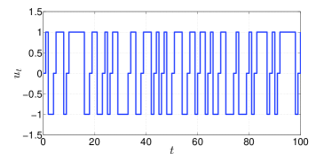
Figure 3: Input realization, Example 3.

Table 2: $h_{m}(\widehat{{\mathcal{I}}}_{F})$, Example 3.

Input / $h_{m}(\widehat{{\mathcal{I}}}_{F})$	$\textsf{log }\textsf{det}(\widehat{{\mathcal{I}}}_{F})$
Optimal	$\mathbf{25.34}(0.01)$
Binary	$24.75(0.01)$
Uniform	$24.38(0.01)$

Table 2 presents the results obtained for each input sequence, where Optimal represents the result for the input sequence obtained from optimizing $\textsf{det}({\mathcal{I}}_{F}^{\operatorname{app}}(\gamma))$. The $95\%$ confidence intervals are given as $\pm$ the value in the parentheses. From these data we conclude that the extended input design method outperforms the experiment results obtained for binary and uniformly distributed samples. Therefore, our new input design method can be successfully employed to design experiments for this nonlinear system.  $\blacksquare$

5 Conclusion

We have presented a new input design method for state space models, which extends existing input design approaches for nonlinear systems. The extension considers a more general model structure, and a new class for the input sequences. The method maximizes a scalar cost function of the information matrix, by optimizing the stationary pmf from which the input sequence is sampled. The elements in the feasible set of the stationary pmf are computed as a convex combination of its extreme points.

Under the assumption of a finite set of possible values for the input, we use graph theoretical tools to compute the information matrix as a convex combination of the information matrices associated with each extreme point. The information matrix for each extreme point is approximated using particle methods, where the information matrix is computed as the covariance of the score function. The numerical examples show that the extended input design method can be successfully used to design experiments for general nonlinear systems.

In a future work we will combine the proposed input design technique with parameter estimation methods, which will allow to simultaneously estimate the parameters and the optimal input for a nonlinear SSM. We will also consider alternative methods based on Gaussian process models for information matrix estimation. This could improve the accuracy and the efficiency in the information matrix estimation method outlined in this paper.

Finally, as with most optimal input design methods, the one proposed in this contribution relies on knowledge of the true system. This difficulty can be overcome by implementing a robust experiment design scheme on top of it (Rojas et al., 2007) or via an adaptive procedure, where the input signal is re-designed as more information is being collected from the system (Rojas et al., 2011). This approach will be also addressed in a future work.

The authors thank to Dr. Fredrik Lindsten for his comments to improve this article.

References

- Boyd and Vandenberghe [2004] S. Boyd and L. Vandenberghe. Convex Optimization. Cambridge University Press, 2004.
- Brighenti et al. [2009] C. Brighenti, B. Wahlberg, and C.R. Rojas. Input design using Markov chains for system identification. In Joint 48th Conference on Decision and Control and 28th Chinese Conference, pages 1557–1562, Shangai, P.R. China, 2009.
- Cappé et al. [2005] O. Cappé, E. Moulines, and T. Rydén. Inference in Hidden Markov Models. Springer, 2005.
- Cock et al. [2013] A. De Cock, M. Gevers, and J. Schoukens. A preliminary study on optimal input design for nonlinear systems. In Proceedings of the IEEE Conference on Decision and Control (CDC’13) (accepted for publication), Florence, Italy, 2013.
- Cox [1958] D.R. Cox. Planning of experiments. New York: Wiley, 1958.
- Dahlin et al. [2013] J. Dahlin, F. Lindsten, and T.B. Schön. Second-order Particle MCMC for Bayesian Parameter Inference. Pre-print, 2013. arXiv:1311.0686v1.
- Del Moral et al. [2006] P. Del Moral, A. Doucet, and A. Jasra. Sequential Monte Carlo samplers. Journal of the Royal Statistical Society: Series B, 68(3):411–436, 2006.
- Doucet and Johansen [2011] A. Doucet and A. Johansen. A tutorial on particle filtering and smoothing: Fifteen years later. In D. Crisan and B. Rozovsky, editors, The Oxford Handbook of Nonlinear Filtering. Oxford University Press, 2011.
- Fedorov [1972] V.V. Fedorov. Theory of optimal experiments. New York: Academic Press, 1972.
- Fisher [1925] R.A. Fisher. Theory of statistical estimation. Mathematical Proceedings of the Cambridge Philosophical Society, 22(05):700–725, 1925.
- Gevers [2005] M. Gevers. Identification for control: from the early achievements to the revival of experiment design. European Journal of Control, 11:1–18, 2005.
- Goodwin and Payne [1977] G.C. Goodwin and R.L. Payne. Dynamic System Identification: Experiment Design and Data Analysis. Academic Press, New York, 1977.
- Gopaluni et al. [2011] R.B. Gopaluni, T.B. Schön, and A.G. Wills. Input design for nonlinear stochastic dynamic systems - A particle filter approach. In Proceedings of the 18th IFAC World Congress, Milano, Italy, 2011.
- Hildebrand and Gevers [2003] R. Hildebrand and M. Gevers. Identification for control: Optimal input design with respect to a worst-case -gap cost function. SIAM Journal of Control Optimization, 41(5):1586–1608, 2003.
- Hjalmarsson and Mårtensson [2007] H. Hjalmarsson and J. Mårtensson. Optimal input design for identification of non-linear systems: Learning from the linear case. In Proceedings of the American Control Conference, pages 1572–1576, New York, United States, 2007.
- Jansson and Hjalmarsson [2005] H. Jansson and H. Hjalmarsson. Input design via LMIs admitting frequency-wise model specifications in confidence regions. IEEE Transactions on Automatic Control, 50(10):1534–1549, October 2005.
- Johnson [1975] D.B. Johnson. Finding all the elementary circuits of a directed graph. SIAM Journal on Computing, 4(1):77–84, March 1975.
- Kitagawa and Sato [2001] G. Kitagawa and S. Sato. Monte carlo smoothing and self-organising state-space model. In A. Doucet, N. de Fretias, and N. Gordon, editors, Sequential Monte Carlo methods in practice, pages 177–195. Springer, 2001.
- Larsson et al. [2010] C. Larsson, H. Hjalmarsson, and C.R. Rojas. On optimal input design for nonlinear FIR-type systems. In Proceedings of the 49th IEEE Conference on Decision and Control, pages 7220–7225, Atlanta, USA, 2010.
- Lindqvist and Hjalmarsson [2000] K. Lindqvist and H. Hjalmarsson. Optimal input design using linear matrix inequalities. In Proceedings of the IFAC Symposium on System Identification, Santa Barbara, California, USA, July 2000.
- Ljung [1999] L. Ljung. System Identification. Theory for the User, 2nd ed. Upper Saddle River, NJ: Prentice-Hall, 1999.
- Louis [1982] T.A. Louis. Finding the observed information matrix when using the EM algorithm. Journal of the Royal Statistical Society: Series B (Statistical Methodology), 44(02):226–233, 1982.
- Olsson et al. [2008] J. Olsson, O. Cappé, R. Douc, and E. Moulines. Sequential Monte Carlo smoothing with application to parameter estimation in nonlinear state space models. Bernoulli, 14(1):155–179, 2008.
- Pitt and Shephard [1999] M.K. Pitt and N. Shephard. Filtering via simulation: Auxiliary particle filters. Journal of the American Statistical Association, 94(446):590–599, 1999.
- Rojas et al. [2007] C.R. Rojas, J.S. Welsh, G.C. Goodwin, and A. Feuer. Robust optimal experiment design for system identification. Automatica, 43(6):993–1008, June 2007.
- Rojas et al. [2011] C.R. Rojas, H. Hjalmarsson, L. Gerencsér, and J. Mårtensson. An adaptive method for consistent estimation of real-valued non-minimum phase zeros in stable LTI systems. Automatica, 47(7):1388–1398, 2011.
- Suzuki and Sugie [2007] H. Suzuki and T. Sugie. On input design for system identification in time domain. In Proceedings of the European Control Conference, Kos, Greece, July 2007.
- Tarjan [1972] R. Tarjan. Depth-First Search and Linear Graph Algorithms. SIAM Journal on Computing, 1(2):146–160, June 1972.
- Valenzuela et al. [2013] P.E. Valenzuela, C.R. Rojas, and H. Hjalmarsson. Optimal input design for dynamic systems: a graph theory approach. In Proceedings of the IEEE Conference on Decision and Control (CDC’13) (accepted for publication), Florence, Italy, 2013. Available in http://arxiv.org/abs/1310.4706.
- Vincent et al. [2009] T.L. Vincent, C. Novara, K. Hsu, and K. Poola. Input design for structured nonlinear system identification. In 15th IFAC Symposium on System Identification, pages 174–179, Saint-Malo, France, 2009.
- Whittle [1973] P. Whittle. Some general points in the theory of optimal experiment design. Journal of Royal Statistical Society, 1:123–130, 1973.
- Zaman [1983] A. Zaman. Stationarity on finite strings and shift register sequences. The Annals of Probability, 11(3):678–684, August 1983.