Non-relativistic Nambu-Goldstone modes
propagating along a skyrmion line

Abstract

We study Nambu-Goldstone (NG) modes or gapless modes propagating along a skyrmion (lump) line in a relativistic and non-relativistic $O(3)$ sigma model, the latter of which describes isotropic Heisenberg ferromagnets. We show for the non-relativistic case that there appear two coupled gapless modes with a quadratic dispersion. In addition to the well-known Kelvin mode consisting of two translational zero modes transverse to the skyrmion line, we show that the other consists of a magnon and dilaton, that is, a NG mode for a spontaneously broken internal $U(1)$ symmetry and a quasi-NG mode for a spontaneously broken scale symmetry of the equation of motion. We find that the commutation relations of Noether charges admit a central extension between the dilatation and phase rotation, in addition to the one between two translations found recently. The counting rule is consistent with the Nielsen-Chadha and Watanabe-Brauner relations only when we take into account quasi-NG modes.

I Introduction

When the symmetry of a Hamiltonian or Lagrangian is broken in the ground state, it is said that the symmetry is spontaneously broken. When a continuous symmetry is spontaneously broken, there appear Nambu-Goldstone (NG) modes as gapless excitations that are dominant at low-energy. It is enough to incorporate these degrees of freedom to construct low-energy effective theories. In relativistic theories, there is a one-to-one correspondence between broken symmetry generators and NG modes, at least for internal symmetries. In the non-relativistic cases, this is not so; In addition to type-I (relativistic) NG modes with a linear dispersion relation each of which corresponds to one broken generator, there are type-II (non-relativistic) NG modes with a quadratic dispersion relation, each of which corresponds to two broken generators Nielsen:1975hm ; Nambu:2004yia ; Watanabe:2011ec ; Watanabe:2012hr ; Hidaka:2012ym . The criteria were summarized as the Watanabe-Brauner relation Watanabe:2011ec stating that when two broken generators, $X_{i}$ and $X_{j}$, do not commute in the ground state, $\left<[X_{i},X_{j}]\right>\neq 0$, they give rise to one type-II NG mode, such as magnons in ferromagnets. This has been recently proved for internal symmetries Watanabe:2012hr ; Hidaka:2012ym .

However, there are no general arguments for spontaneously broken space-time symmetry (see, e.g., Refs. Watanabe:2013iia ; Hayata:2013vfa ; Brauner:2014aha for recent studies). In the presence of topological defects, space-time symmetries are spontaneously broken. For instance, it has been long known that there appears only one type-II NG mode, known as a Kelvin mode, or Kelvon if quantized, corresponding to two translational symmetries spontaneously broken in the presence of a quantized vortex in superfluids or a skyrmion (lump) Polyakov:1975yp in ferromagnets, while there are two type-I NG modes in the case of a relativistic string (see, e.g., Ref. Kobayashi:2013gba ; Eto:2013hoa for a vortex and Ref. skyrmion-dynamics for a skyrmion). Recently, Watanabe and Murayama Watanabe:2014pea have found

$$\left[P_{x},P_{y}\right]=B\neq 0$$ (1)

in the background of a quantized vortex or a skyrmion line, where $P_{x}$ and $P_{y}$ are the Noether charges of translations perpendicular to the skyrmion or vortex line, and $B$ is a topological charge for the skyrmion or vortex line. The two translational generators give one type-II NG mode, a Kelvon, to be consistent with the Watanabe-Brauner relation Watanabe:2011ec . In our previous work Kobayashi:2014xua , we have further found

$$\left[P_{x},\Theta\right]=W\neq 0$$ (2)

in the background of a domain wall Abraham:1992vb (a magnetic domain wall in ferromagnets Tatara:2008 ), where $P_{x}$ is the Noether charge of the translation perpendicular to the wall, $\Theta$ is the Noether charge of an internal $U(1)$ symmetry, and $W$ is a topological charge of the domain wall. A similar result has been obtained in Ref. Watanabe:2014zza for a domain wall in two-component Bose-Einstein condensates Takeuchi:2013mwa . In the relativistic case, the two operators in Eq. (2) commute and there are two type-I NG modes. The latter non-commutative relation (2) resembles supersymmetry algebras in the presence of Bogomol’nyi-Prasad-Sommerfield (BPS) solitons in supersymmetric field theories Witten:1978mh ; Dvali:1996bg and $p$-branes in supergravity and string theory de Azcarraga:1989gm .

In this paper, in addition to Eq. (1) for the translational modes in the presence of a skyrmion line, we show

$$\left[D,\Theta+M_{12}\right]\neq 0$$ (3)

where $D$ is the Noether charge of a dilatation and $M_{12}$ is the Noether charge of a rotation around the $z$–axis along which the skyrmion line is placed. The skyrmion solution has four moduli $X$, $Y$, $\theta$, and $R$. While $X$, $Y$ and $\theta$ are NG modes of two translations and the internal $U(1)$ symmetry, respectively, we point out that a dilaton $R$ is a quasi-NG mode Weinberg:1972fn , which appears when a symmetry of the equation of motion, but not that of the Lagrangian or action, is spontaneously broken. By constructing the low-energy effective field theory on a 1+1 dimensional skyrmion world-sheet via the moduli approximation Manton:1981mp , we find that the dilaton $R$ and the $U(1)$ NG mode (magnon) $\theta$ are coupled to give rise to one type-II gapless mode, which is consistent with the Watanabe-Brauner relation only when we count quasi-NG modes, while, in the relativistic case, the dilaton and the $U(1)$ NG mode appear independently as type-I (quasi-)NG modes. We further study fluctuations around the solution in the Bogoliubov analysis and find the same result. We also consider the effects of explicit breaking terms for the scale symmetry, that is the baby skyrme term and a potential term. In the presence of these terms, the skyrmions are known as baby skyrmions Piette:1994ug . We show that these terms introduce a potential term for the dilaton in the effective Lagrangian. In the relativistic case, the dilaton becomes massive and the magnon remains massless as expected. In the non-relativistic case, on the other hand, the magnon-dilaton becomes a type-I NG mode.

II Nonlinear sigma models and skyrmions

We consider the following relativistic and non-relativistic $\mathbb{C}P^{1}$ Lagrangian densities $\mathcal{L}_{\mathrm{rel}}$ and $\mathcal{L}_{\mathrm{nrel}}$,

$$\mathcal{L}_{\mathrm{rel}}=\frac{|\dot{u}|^{2}-|\nabla u|^{2}}{(1+|u|^{2})^{2}},\quad\mathcal{L}_{\mathrm{nrel}}=\frac{i(u^{\ast}\dot{u}-\dot{u}^{\ast}u)}{2(1+|u|^{2})}-\frac{|\nabla u|^{2}}{(1+|u|^{2})^{2}},$$ (4)

where, $u\in\mathbb{C}$ is the complex projective coordinate of $\mathbb{C}P^{1}$, defined as $\phi^{T}=(1,u)^{T}/\sqrt{1+|u|^{2}}$ with normalized two complex scalar fields $\phi=(\phi_{1},\phi_{2})^{T}$. The non-relativistic Lagrangian $\mathcal{L}_{\mathrm{nrel}}$ is obtained by taking the non-relativistic limit of $\mathcal{L}_{\mathrm{rel}}$ (see Appendix A of Ref. Kobayashi:2014xua ). $\mathcal{L}_{\mathrm{rel}}$ and $\mathcal{L}_{\mathrm{nrel}}$ can be rewritten as $O(3)$ nonlinear sigma models,

$$\begin{split}\mathcal{L}_{\mathrm{rel}}=\frac{1}{4}\{|\dot{\bm{n}}|^{2}-|\nabla\bm{n}|^{2}\},\quad\mathcal{L}_{\mathrm{nrel}}=\frac{\dot{n}_{1}n_{2}-n_{1}\dot{n}_{2}}{2(1+n_{3})}-\frac{1}{4}|\nabla\bm{n}|^{2},\end{split}$$ (5)

under the Hopf map for a three-vector of real scalar fields $\bm{n}\equiv\phi^{\dagger}\bm{\sigma}\phi$ with the Pauli matrices $\bm{\sigma}$. These models describe isotropic Heisenberg ferromagnets. In this paper, we use the $\mathbb{C}P^{1}$ model notation.

The Lagrangians $L_{\mathrm{rel}}=\int d^{3}x\>\mathcal{L}_{\mathrm{rel}}$ and $L_{\mathrm{nrel}}=\int d^{3}x\>\mathcal{L}_{\mathrm{nrel}}$ are invariant under a global $SU(2)$ rotation of $\phi$, the Poincaré (for $L_{\mathrm{rel}}$) or Galilean (for $L_{\mathrm{nrel}}$) transformation. In the vacuum of the system, i.e., the arbitrary uniform $u$, the internal $SU(2)$ symmetry is spontaneously broken down to a $U(1)$ symmetry with the identification of the global phase of $\phi$ (phase of $\phi_{1}$). The vacuum manifold is, therefore, isomorphic to $\mathcal{M}_{1}\simeq SU(2)/U(1)\simeq\mathbb{C}P^{1}\simeq S^{2}$.

The dynamics of $u$ can be described by the Euler-Lagrange equation for $\mathcal{L}_{\mathrm{rel}}$ and $\mathcal{L}_{\mathrm{nrel}}$:

$$\begin{split}&(1+|u|^{2})\ddot{u}-2u^{\ast}\dot{u}^{2}\stackrel{{\scriptstyle\mathrm{rel}}}{{=}}(1+|u|^{2})\nabla^{2}u-2u^{\ast}(\nabla u)^{2},\\ &-i(1+|u|^{2})\dot{u}\stackrel{{\scriptstyle\mathrm{nrel}}}{{=}}(1+|u|^{2})\nabla^{2}u-2u^{\ast}(\nabla u)^{2},\end{split}$$ (6)

where $\stackrel{{\scriptstyle\mathrm{rel}}}{{=}}$ and $\stackrel{{\scriptstyle\mathrm{nrel}}}{{=}}$ correspond to dynamics derived from $\mathcal{L}_{\mathrm{rel}}$ and $\mathcal{L}_{\mathrm{nrel}}$, respectively. The equations of motion (6) enjoy an additional symmetry of a scaling transformation $(t,x,y,z)\to(st,sx,sy,sz)$ for the relativistic case and $(t,x,y,z)\to(s^{2}t,sx,sy,sz)$ for the non-relativistic case with $s\in{\mathbb{R}}^{+}-\{0\}\simeq{\mathbb{R}}$. These are not symmetry of the Lagrangians or the actions.

We next consider a static skyrmion line solution. A straight skyrmion line solution parallel to the $z$-axis is Polyakov:1975yp

$$u_{0}(x,y,z)=\frac{\exp\big{\{}i\big{(}\tan^{-1}\frac{y-Y}{x-X}+\theta\big{)}\big{\}}\sqrt{(x-X)^{2}+(y-Y)^{2}}}{R_{0}+R},$$ (7)

where $R_{0}\in\mathbb{R}$ is the characteristic radius of the skyrmion line, and $X,Y\in\mathbb{R}$, $\theta\ (0\leq\theta<2\pi)$, and $R\in\mathbb{R}$ are the translational, phase, and dilatation moduli of the skyrmion line respectively. The tension of the skyrmion line (the energy per unit area) is

$$T=\int dxdy\>\frac{|\nabla u_{0}|^{2}}{(1+|u_{0}|^{2})^{2}}=2\pi,$$ (8)

independent of $X$, $Y$, $\theta$, and $R$. The $U(1)$ phase rotation of $u$, the translation $\mathbb{R}^{2}_{txy}$ inside the $xy$–plane, and the dilatation $\mathbb{R}_{dxy}$ inside the $xy$–plane are spontaneously broken in the vicinity of the skyrmion line. The four moduli $X$, $Y$, $\theta$, and $R$ in Eq. (7) are regarded as NG modes corresponding to $\mathbb{R}^{2}_{txy}$, $U(1)$ and $\mathbb{R}_{dxy}$, respectively, localized in the vicinity of the skyrmion line rotational-symmetry . The NG modes $X$ and $Y$ are the translational modes, which are called as Kelvin waves of the skyrmion line in the non-relativistic case. The NG mode $\theta$ may be called as the localized magnon. We call $R$ as the dilaton, associated with the spontaneously broken $\mathbb{R}_{dxy}$. This $\mathbb{R}_{dxy}$ is merely a symmetry of the equation of motion but not that of the full theory. Consequently $R$ is a so-called quasi-NG mode Weinberg:1972fn but not a genuine NG mode, which is gapless at least classically, see, e.g., Ref. Uchino:2010pf for an example of a quasi-NG mode in condensed matter physics. The dilaton $R$ is similar to the localized varicose mode excited along a superfluid vortex in terms of the radius wave of the string Simula:2008 , but it has a gap in the absence of the dilatational symmetry.

III Low-energy effective theory of a skyrmion line

We next discuss the dynamics of the localized NG modes in the vicinity of the skyrmion line, by constructing the effective theory on a skyrmion line using the moduli approximation Manton:1981mp . Let us introduce the $z$ and $t$ dependences of the moduli in Eq. (7) as $X(z,t)$, $Y(z,t)$, $\theta(z,t)$, and $R(z,t)$:

$$u(x,y,z)=\frac{\exp\big{[}i\big{\{}\tan^{-1}\frac{y-Y(z,t)}{x-X(z,t)}+\theta(z,t)\big{\}}\big{]}\sqrt{\{x-X(z,t)\}^{2}+\{y-Y(z,t)\}^{2}}}{R_{0}+R(z,t)}.$$ (9)

By inserting Eq. (9) back into Eq. (4), the two effective Lagrangians $L^{\mathrm{eff}}_{\mathrm{rel}}$ and $L^{\mathrm{eff}}_{\mathrm{nrel}}$ defined as $L^{\mathrm{eff}}_{\mathrm{rel}}=\int_{-L}^{L}dx\>\int_{-\sqrt{L^{2}-x^{2}}}^{\sqrt{L^{2}-x^{2}}}dy\>\mathcal{L}_{\mathrm{rel}}$ and $L^{\mathrm{eff}}_{\mathrm{nrel}}=\int_{-L}^{L}dx\>\int_{-\sqrt{L^{2}-x^{2}}}^{\sqrt{L^{2}-x^{2}}}dy\>\mathcal{L}_{\mathrm{nrel}}$ can be calculated, to yield

$$\begin{split}&L^{\mathrm{eff}}_{\mathrm{rel}}=\pi(\dot{X}^{2}+\dot{Y}^{2}-X_{z}^{2}-Y_{z}^{2})+2\pi\log\bigg{(}\frac{L}{R_{0}}\bigg{)}(R_{0}^{2}\dot{\theta}^{2}+\dot{R}^{2}-R_{0}^{2}\theta_{z}^{2}-R_{z}^{2})\\ &\phantom{\frac{L^{\mathrm{eff}}_{\mathrm{rel}}}{\pi}=}-2\pi+O(\partial_{z}^{3}),\\ &L^{\mathrm{eff}}_{\mathrm{nrel}}=-\pi L^{2}\dot{\theta}+\pi(\dot{X}Y-X\dot{Y}-X_{z}^{2}-Y_{z}^{2})+2\pi\log\bigg{(}\frac{L}{R_{0}}\bigg{)}(2R_{0}\dot{\theta}R-R_{0}^{2}\theta_{z}^{2}-R_{z}^{2})\\ &\phantom{\frac{L^{\mathrm{eff}}_{\mathrm{nrel}}}{\pi}=}-2\pi+O(\partial_{z}^{3}),\end{split}$$ (10)

up to the quadratic order in derivatives.

The low-energy dynamics of $X$, $Y$, $\theta$, and $R$ derived from the Euler-Lagrange equation becomes

$$\ddot{X}\stackrel{{\scriptstyle\mathrm{rel}}}{{=}}X_{zz},\quad\ddot{Y}\stackrel{{\scriptstyle\mathrm{rel}}}{{=}}Y_{zz},\quad\ddot{\theta}\stackrel{{\scriptstyle\mathrm{rel}}}{{=}}\theta_{zz},\quad\ddot{R}\stackrel{{\scriptstyle\mathrm{rel}}}{{=}}R_{zz},$$ (11a)

$$\dot{X}\stackrel{{\scriptstyle\mathrm{nrel}}}{{=}}-Y_{zz},\quad\dot{Y}\stackrel{{\scriptstyle\mathrm{nrel}}}{{=}}X_{zz},\quad R_{0}\dot{\theta}\stackrel{{\scriptstyle\mathrm{nrel}}}{{=}}-R_{zz},\quad\dot{R}\stackrel{{\scriptstyle\mathrm{nrel}}}{{=}}R_{0}\theta_{zz}.$$ (11b)

For the relativistic case, all dynamics of $X$, $Y$, $\theta$ and $R$ are independent of each other, giving linear dispersions:

$$\omega_{\mathrm{rel}}=\pm|\bm{k}|,$$ (12)

with the frequencies $\omega_{\mathrm{rel}}$, and the wave number $k$. Oscillations $X$ and $Y$ of the skyrmion line into the $x$ and $y$–directions, a localized magnon $\theta$ and a dilaton $R$ independently propagate along the $z$-axis.

Being different from the relativistic case, there are two different coupled modes, $X$ and $Y$, and $\theta$ and $R$ in the non-relativistic case. Typical solutions of Eq. (11b) are

$$X=A_{(XY)\pm}\sin(kz\mp\omega_{\mathrm{nrel}}t+\delta_{(XY)\pm}),\quad Y=\mp A_{(XY)\pm}\cos(kz\mp\omega_{\mathrm{nrel}}t+\delta_{(XY)\pm}),$$ (13a)

$$\theta=A_{(\theta R)\pm}\sin(kz\mp\omega_{\mathrm{nrel}}t+\delta_{(\theta R)\pm}),\quad R=\mp R_{0}A_{(\theta R)\pm}\cos(kz\mp\omega_{\mathrm{nrel}}t+\delta_{(\theta R)\pm}),$$ (13b)

where $A_{(XY),(\theta R)\pm}\in\mathbb{R}$ and $\delta_{(XY),(\theta R)\pm}\in\mathbb{R}$ are arbitrary constants. Waves of $X$ and $Y$ couple and propagate as a spiral Kelvin wave, and $\theta$ and $R$ couple to each other and propagate as a coupled magnon-dilaton, both with a quadratic dispersion

$$\omega_{\mathrm{nrel}}=k^{2}.$$ (14)

For the upper and lower signs in Eqs. (13a) and (13b), each coupled NG mode propagates in the direction parallel and anti-parallel to $z$–axis, respectively. In contrast to the Kelvin wave in Eq. (13a) which are combinations of two translational modes in real space, the localized coupled magnon-dilaton mode in Eq. (13b) is a combination of the phase mode of the internal degrees of freedom and the dilatation in real space. Figure 1 shows the schematic picture of coupled localized magnon-dilaton mode for Eq. (13b) movie .

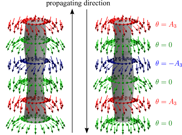
Figure 1: (Color online) Schematic picture of the localized coupled magnon-dilaton for Eq. (13b). The arrows show the direction of $\bm{n}=\phi^{\dagger}\bm{\sigma}\phi$ with $\phi^{T}=(1,u)^{T}/\sqrt{1+|u|^{2}}$ and their colors shows the value of $\theta$. The transparent surface shows the isosurface for $|u|=0$ ($n_{3}=0$). For left (right) figures, the coupled localized magnon-dilaton propagate in the upper (lower) direction.

IV Linear response theory

Linear response theory is another technique to study the dynamics of the gapless modes $X,Y,\theta,R$. Let us consider the ansatz of the straight skyrmion line solution and its fluctuation: $u=u_{0}+\delta u=u_{0}+a_{+}e^{i(kz-\omega t)}+a_{-}^{\ast}e^{-i(kz-\omega t)}$. By inserting this ansatz into the dynamical equation (6), the Bogoliubov-de Gennes equations are obtained,

$$\begin{split}&\omega_{\mathrm{rel}}^{2}a_{\pm}\stackrel{{\scriptstyle\mathrm{rel}}}{{=}}\bigg{\{}(k^{2}-\nabla_{\bm{r}}^{2})+\frac{4(r\partial_{r}\pm i\partial_{\theta})}{r^{2}+R_{0}^{2}}\bigg{\}}a_{\pm}+O(a_{\pm}^{2}),\\ &\omega_{\mathrm{nrel},\pm}a_{\pm}\stackrel{{\scriptstyle\mathrm{nrel}}}{{=}}\pm\bigg{\{}(k^{2}-\nabla_{\bm{r}}^{2})+\frac{4(r\partial_{r}\pm i\partial_{\theta})}{r^{2}+R_{0}^{2}}\bigg{\}}a_{\pm}+O(a_{\pm}^{2}),\end{split}$$ (15)

up to the linear order of $a_{\pm}$. Here, $\nabla_{\bm{r}}=(\partial_{x},\partial_{y})$ denotes the derivative in the $xy$–plane. By expanding $a_{\pm}$ as $a_{\pm}=\sum_{l}a_{\pm,l}e^{il\phi}$, we obtain

$$\begin{split}&\omega_{\mathrm{rel}}^{2}a_{\pm,l}\stackrel{{\scriptstyle\mathrm{rel}}}{{=}}\bigg{\{}(k^{2}-\partial_{r}^{2}-\partial_{r}/r+l^{2}/r^{2})+\frac{4(r\partial_{r}\mp l)}{r^{2}+R_{0}^{2}}\bigg{\}}a_{\pm,l}+O(a_{\pm}^{2}),\\ &\omega_{\mathrm{nrel},\pm}a_{\pm,l}\stackrel{{\scriptstyle\mathrm{nrel}}}{{=}}\pm\bigg{\{}(k^{2}-\partial_{r}^{2}-\partial_{r}/r+l^{2}/r^{2})+\frac{4(r\partial_{r}\mp l)}{r^{2}+R_{0}^{2}}\bigg{\}}a_{\pm,l}+O(a_{\pm}^{2}).\end{split}$$ (16)

There are two characteristic solutions related to the Kelvin wave, localized magnon, and dilaton: $a_{\pm,0}=1$ and $a_{\pm,1}=r/R_{0}$, and eigenvalues are $\omega_{\mathrm{rel}}^{2}=k^{2}$ and $\omega_{\mathrm{nrel,\pm}}=\pm k^{2}$. For the relativistic case, NG modes for $X$, $Y$, $\theta$, and $R$ are obtained as

$$\begin{split}&X\ :\ \delta u=A_{X\pm}(a_{+,0}e^{i(kz\mp kt+\delta_{X\pm})}+a_{-,0}e^{-i(kz\mp kt+\delta_{X\pm})}),\\ &Y\ :\ \delta u=A_{Y\pm}(a_{+,0}e^{i(kz\mp kt+\delta_{Y\pm})}-a_{-,0}e^{-i(kz\mp kt+\delta_{Y\pm})}),\\ &\theta\ :\ \delta u=A_{\theta\pm}(a_{+,1}e^{i\phi}e^{i(kz\mp kt+\delta_{\theta\pm})}-a_{-,1}e^{i\phi}e^{-i(kz\mp kt+\delta_{\theta\pm})}),\\ &R\ :\ \delta u=A_{R\pm}(a_{+,1}e^{i\phi}e^{i(kz\mp kt+\delta_{R\pm})}+a_{-,1}e^{i\phi}e^{-i(kz\mp kt+\delta_{R\pm})}),\end{split}$$ (17)

with arbitrary constant $A_{X,Y,\theta,R\pm},\delta_{X,Y,\theta,R\pm}\in\mathbb{R}$. The upper (lower) sign in Eq. (17) shows the NG modes propagating in the direction parallel (anti-parallel) to the $z$–axis. For non-relativistic case, the coupled NG modes for, $(X,Y)$, and $(\theta,R)$ are obtained as

$$\begin{split}&(X,Y)\ :\ \delta u=A_{(XY)\pm}a_{\pm,0}e^{\pm i(kz\mp k^{2}t+\delta_{(XY)\pm})},\\ &(\theta,R)\ :\ \delta u=A_{(\theta R)\pm}a_{\pm,1}e^{i\phi}e^{\pm i(kz\mp k^{2}t+\delta_{(\theta R)\pm})}.\end{split}$$ (18)

We shortly note that there are countably infinite number of gapless solutions to the Bogoliubov-de Gennes equation (15), $a_{\pm,n}=r^{n}/R_{0}^{n}$ ($n\in\mathbb{Z}_{0}^{+})$ and corresponding zero modes $\omega_{\mathrm{rel}}^{2}=k^{2}$ and $\omega\in{nrel,\pm}=\pm k^{2}$ besides the present solutions $a_{\pm,0}$ and $a_{\pm,1}$. Solutions for $n=0,1,2$ correspond to the (quasi-)NG modes; i.e., $a_{\pm,0}$ corresponds to the Kelvin waves, $a_{\pm,1}$ corresponds to the localized magnon and dilaton, and $a_{\pm,2}$ corresponds to the bulk magnon far from the skyrmion line, for which we have not discussed in this paper. The other solutions, $a_{\pm,n\neq 0,1,2}$, do not originate from any symmetry of the Lagrangians and cannot be regarded as NG modes. We will soon discuss this in detail elsewhere.

V Commutation relation

By the two techniques of the effective theory with the moduli approximation and the linear-response theory, we have shown the independence of the four gapless modes in the presence of the skyrmion line– the two translational modes, the localized magnon, and the dilaton. They are independent of each other with the linear dispersion relations (12) for the relativistic theory with $\mathcal{L}_{\mathrm{rel}}$, while the coupled spiral Kelvin wave and the coupled localized magnon-dilaton are formed showing the quadratic dispersion relations (14) for the non-relativistic theory with $\mathcal{L}_{\mathrm{nrel}}$. These modes are (quasi-)NG modes appearing as a consequence of the spontaneous breaking continuous symmetries; the $\mathbb{R}_{txy}^{2}$ translational symmetry for Kelvin waves, the $U(1)$ symmetry for the localized magnon, and the two-dimensional $\mathbb{R}_{dxy}$ scaling symmetry for the dilaton. The Lorentz invariance in the relativistic model supports that the number of (quasi-)NG modes is equivalent to that of symmetry generators $N_{\mathrm{BG}}$ corresponding to spontaneously broken symmetries, and all (quasi-)NG modes are type-I for the linear dispersion (12). Without the Lorentz invariance, there appear not only type I (quasi-)NG modes but also type II (quasi-)NG modes with the quadratic dispersion and the relation between the number of (quasi-)NG modes and $N_{\mathrm{BG}}$ becomes more complicated. In both cases, the numbers of (quasi-)NG modes saturates the equality of the Nielsen-Chadha inequality Nielsen:1975hm , $N_{\mathrm{I}}+2N_{\mathrm{II}}\geq N_{\mathrm{BG}}$, where $N_{\mathrm{I}}$ and $N_{\mathrm{II}}$ are the total numbers of the type-I NG modes and the type-II NG modes. In the case of internal symmetries, it has been shown in Refs. Watanabe:2012hr ; Hidaka:2012ym that the equality of the Nielsen-Chadha inequality is saturated as the Watanabe-Brauner’s relation Watanabe:2011ec ,

$$N_{\mathrm{BG}}-N_{\mathrm{NG}}=\frac{1}{2}\mathrm{rank}\rho,\quad\rho_{i,j}=\lim_{V\to\infty}\frac{1}{V}\int d^{3}\bm{x}[\Omega_{i},\Omega_{j}]\Big{|}_{u=u_{0}}.$$ (19)

Here, $N_{\mathrm{NG}}=N_{\mathrm{I}}+N_{\mathrm{II}}$ is the total number of NG modes, $V$ is the volume of the system, $\Omega_{i}$ is the Noether charge or a generator of broken symmetries, and $[\cdot,\cdot]$ is a commutator or the Poisson bracket in the classical level. We see that a mismatching $N_{\mathrm{BG}}\neq N_{\mathrm{NG}}$ takes place when commutators of broken generators are non-vanishing in the ground states in non-relativistic theories. This relation has been proven for cases of the bulk magnons (two internal symmetries) and the Kelvin wave (two space-time symmetries) in the massless $\mathbb{C}P^{1}$ model for the isotropic Heisenberg ferromagnet Watanabe:2014pea . It has been also proved for the translational and internal $U(1)$ zero modes in the background of a domain wall in the massive $\mathbb{C}P^{1}$ model for the Heisenberg ferromagnet with one easy axis Kobayashi:2014xua . As the case of a domain wall in Ref. Kobayashi:2014xua , the two broken generators corresponding to the coupled localized magnon-dilaton, that is, the internal $U(1)$ symmetry and translational symmetry, intuitively commute, because underlying symmetries are the direct product and are independent of each other, i.e., $U(1)\times\mathbb{R}_{dxy}$. In order to check whether the relation (19) also holds in our case or not, let us directly calculate the commutation relation between Noether charges of symmetry generatros of the localized magnon and the dilaton.

Before calculating the commutator for the localized magnon and the dilatation mode, we briefly overview the commutator of the two translations for the spiral Kelvin wave Watanabe:2014pea which also intuitively commute with each other. Let us define the momenta $v$ conjugate to $u$ as

$$v\stackrel{{\scriptstyle\mathrm{rel}}}{{=}}\frac{\partial\mathcal{L}_{\mathrm{rel}}}{\partial\dot{u}}=\frac{\dot{u}^{\ast}}{(1+|u|^{2})^{2}},\quad v\stackrel{{\scriptstyle\mathrm{nrel}}}{{=}}\frac{\partial\mathcal{L}_{\mathrm{nrel}}}{\partial\dot{u}}=\frac{iu^{\ast}}{2(1+|u|^{2})}.$$ (20)

Then, the Noether’s charges for the translations for $x$ and $y$–directions are obtained as

$$P_{x}=\int d^{2}x\>J^{0}_{X},\quad J^{0}_{X}=u_{x}v,\qquad P_{y}=\int d^{2}x\>J^{0}_{Y},\quad J^{0}_{Y}=u_{x}v.$$ (21)

The commutator between $P_{x}$ and $P_{y}$ can be calculated from $[u(x_{1},y_{1}),v(x_{2},y_{2})]=\delta(x_{1}-x_{2})\delta(y_{1}-y_{2})\equiv\delta^{2}(\bm{x}_{1}-\bm{x}_{2})$, to yield

$$\begin{split}[P_{x},P_{y}]&=\int d^{2}x_{1}\>\int d^{2}x_{2}\>[J^{0}_{X}(x_{1},y_{1}),J^{0}_{Y}(x_{2},y_{2})]\\ &=\int d^{2}x_{1}\>\int d^{2}x_{2}\>[u_{x_{1}}(x_{1},y_{1})v(x_{1},y_{1}),u_{y_{2}}(x_{2},y_{2})v(x_{2},y_{2})]\\ &=\int d^{2}x_{1}\>\int d^{2}x_{2}\>\{u_{x_{1}}(x_{1},y_{1})[v(x_{1},y_{1}),u_{y_{2}}(x_{2},y_{2})]v(x_{2},y_{2})\\ &\phantom{=i\int d^{2}x_{1}\>\int d^{2}x_{2}\>\{}+u_{y_{2}}(x_{2},y_{2})[u_{x_{1}}(x_{1},y_{1}),v(x_{2},y_{2})]v(x_{1},y_{1})\}\\ &=\int d^{2}x_{1}\>\int d^{2}x_{2}\>\{u_{x_{1}}(x_{1},y_{1})v_{y_{2}}(x_{2},y_{2})-u_{y_{2}}(x_{2},y_{2})v(x_{1},y_{1})\}\delta^{2}(\bm{x}_{1}-\bm{x}_{2})\\ &=\int d^{2}x\>\{u_{x}(x,y)v_{y}(x,y)-u_{y}(x,y)v(x,y)\}\\ &=\int d^{2}x\>\frac{u_{r}v_{\phi}-u_{\phi}v_{r}}{r},\end{split}$$ (22)

with the cylinderical coordinate $(r,\phi)$.

The commutator vanishes for the relativistic case because of $v=0$ ($\dot{u}=0$), implying two type I NG modes.

For the non-relativistic case, the commutator becomes Watanabe:2014pea

$$\begin{split}[P_{x},P_{y}]=\int d^{2}x\>\frac{u_{r}v_{\phi}-u_{\phi}v_{r}}{r}=\int d^{2}x\>b=B\neq 0,\end{split}$$ (23)

where $b$ and $B$ are the topological charge density and the total topological charge of the skyrmion line:

$$b=u_{x}v_{y}-u_{y}v_{x}=\frac{u_{r}v_{\phi}-u_{\phi}v_{r}}{r}=\frac{R_{0}^{2}}{(r^{2}+R_{0}^{2})^{2}},\quad B=\int_{0}^{\infty}dr\>\int_{0}^{2\pi}d\theta\>rb=\pi.$$ (24)

In the last equalities in (24), we have used the background of a single skyrmion line $u=u_{0}=re^{i\phi}/R_{0}$.

We next calculate the commutator for the localized magnon and dilaton. The Noether’s charges for the phase shift and the dilatation are obtained as

$$\Theta=\int d^{2}x\>J^{0}_{\theta},\quad J^{0}_{\theta}=iuv,$$ (25)

$$D=\int d^{2}x\>J^{0}_{R},\quad J^{0}_{R}=(xu_{x}+yu_{y})v,$$ (26)

respectively. The commutator between them reads

$$\begin{split}[D,\Theta]&=\int d^{2}x_{1}\>\int d^{2}x_{2}\>[J^{0}_{D}(x_{1},y_{1}),J^{0}_{\theta}(x_{2},y_{2})]\\ &=i\int d^{2}x_{1}\>\int d^{2}x_{2}\>[\{x_{1}u_{x_{1}}(x_{1},y_{1})+y_{1}u_{y_{1}}(x_{1},y_{1})\}v(x_{1},y_{1}),u(x_{2},y_{2})v(x_{2},y_{2})]\\ &=i\int d^{2}x_{1}\>\int d^{2}x_{2}\>[x_{2}\{u(x_{1},y_{1})[u_{x_{2}}(x_{2},y_{2}),v(x_{1},y_{1})]v(x_{2},y_{2})\\ &\phantom{=i\int d^{2}x_{1}\>\int d^{2}x_{2}\>[x_{2}\{}+u_{x_{2}}(x_{2},y_{2})[v(x_{2},y_{2}),u(x_{1},y_{1})]v(x_{1},y_{1})\}\\ &\phantom{=i\int d^{2}x_{1}\>\int d^{2}x_{2}\>[}+y_{2}\{u(x_{1},y_{1})[u_{y_{2}}(x_{2},y_{2}),v(x_{1},y_{1})]v(x_{2},y_{2})\\ &\phantom{=i\int d^{2}x_{1}\>\int d^{2}x_{2}\>[+y_{2}\{}+u_{y_{2}}(x_{2},y_{2})[v(x_{2},y_{2}),u(x_{1},y_{1})]v(x_{1},y_{1})\}].\\ &=-i\int d^{2}x_{1}\>\int d^{2}x_{2}\>[x_{2}\{u(x_{1},y_{1})v_{x_{2}}(x_{2},y_{2})+u_{x_{2}}(x_{2},y_{2})v(x_{1},y_{1})\}\\ &\phantom{=-i\int d^{2}x_{1}\>\int d^{2}x_{2}\>[}+y_{2}\{u(x_{1},y_{1})v_{y_{2}}(x_{2},y_{2})+u_{y_{2}}(x_{2},y_{2})v(x_{1},y_{1})\}\\ &\phantom{=-i\int d^{2}x_{1}\>\int d^{2}x_{2}\>[}+2u(x_{1},y_{1})v(x_{2},y_{2})]\delta^{2}(\bm{x}_{1}-\bm{x}_{2})\\ &=-i\int d^{2}x\>[r\{u_{r}(r,\phi)v(r,\phi)+u(r,\phi)v_{r}(r,\phi)\}+2u(r,\phi)v(r,\phi)].\end{split}$$ (27)

For the non-relativistic case, the commutator becomes

$$\begin{split}[D,\Theta]=\int d^{2}x\>\frac{r^{2}(r^{2}+2R_{0}^{2})}{(r^{2}+R_{0}^{2})^{2}}=\int d^{2}x\>r^{2}\bigg{(}b+\frac{1}{r^{2}+R_{0}^{2}}\bigg{)}\neq 0,\end{split}$$ (28)

while it vanishes for the relativistic case.

The ansatz in Eq. (9) with $X=Y=0$,

$$u(r,\phi,z)=\frac{r\exp\{i(\phi+\theta)\}}{R_{0}+R},$$ (29)

implies that the localized magnon $\theta$ can be induced not only by the phase shift of $u$, $u\to ue^{i\theta}$, but also by a spatial rotation along $z$–axis, $\phi\to\phi+\theta$. Therefore, we further calculate the commutator between the spatial rotation and the dilatation. The Noether’s charge for the rotation is

$$M_{12}=\int d^{2}x\>J_{\phi}^{0},\quad J_{\phi}^{0}=(xu_{y}-yu_{x})v.$$ (30)

In addition to Eq. (27), the commutator becomes

$$\begin{split}[D,M_{12}]&=\int d^{2}x_{1}\>\int d^{2}x_{2}\>[J^{0}_{D}(x_{1},y_{1}),J^{0}_{\phi}(x_{2},y_{2})]\\ &=\int d^{2}x\>[(x^{2}+y^{2})\{u_{x}(x_{2},y_{2})v_{y}(x_{1},y_{1})-u_{y}(x_{1},y_{1})v_{x}(x_{2},y_{2})\}\\ &\phantom{=\int d^{2}x\>[}+2\{yu_{x}(x_{1},y_{1})-xu_{y}(x_{2},y_{2})\}v(x,y)\}\\ &=\int d^{2}x\>[r\{u_{r}(r,\phi)v_{\phi}(r,\phi)-u_{\phi}(r,\phi)v_{r}(r,\phi)\}-2u_{\phi}(r,\phi)v(r,\phi)]\\ &=\int d^{2}x\>r^{2}\bigg{(}b+\frac{1}{r^{2}+R_{0}^{2}}\bigg{)}\\ &=[D,\Theta].\end{split}$$ (31)

The fact $[D,\Theta-M_{12}]=0$ implies that $u_{0}$ is invariant under a simultaneous action of the phase shift $u\to ue^{i\theta}$ and the spatial rotation $\phi\to\phi-\theta$. Therefore, we find an independent non-vanishing commutation relation

$$\left[D,\Theta+M_{12}\right]=2\int d^{2}x\>r^{2}\bigg{(}b+\frac{1}{r^{2}+R_{0}^{2}}\bigg{)}\neq 0,$$ (32)

which is consistent with our result for the coupled localized magnon-dilaton.

VI The explicit breaking term for the scale symmetry: the case of baby skyrmions

Here, we briefly investigate the effect of a small explicit breaking term for the scaling symmetry. One of the simple additional terms, $\mathcal{L}_{\mathrm{add}}$, that explicitly breaks the scaling symmetry is

$$\mathcal{L}_{\mathrm{add}}=-\frac{\kappa\{(|\nabla u|^{2})^{2}-|(\nabla u)^{2}|^{2}\}}{(1+|u|^{2})^{4}}-\frac{2\beta^{2}}{1+|u|^{2}}.$$ (33)

Here, the first and second terms are the baby skyrme term and the potential term (corresponding to the magnetic field along the $n_{3}$ axis in ferromagnets), by which the skyrmion tends to expand and shrink, respectively. In the presence of both terms, the skyrmions are known as baby skyrmions with a fixed size Piette:1994ug .

Here, we suppose that the parameters $\kappa$ and $\beta$ are small, and treat the additional terms in Eq. (33) as small perturbations. We can assume the configuration in Eq. (9) is unchanged at the leading order. Minimizing the energy for the configuration in Eq. (9), the size $R_{0}$ is determined by

$$\kappa=3\beta^{2}R_{0}^{4}\log(L/R_{0}).$$ (34)

With small $\kappa$ and $\beta$, the effective Lagrangians for $R$ and $\theta$ become

$$\begin{split}&L_{\mathrm{rel}}^{\mathrm{eff}}+\int dxdy\>\mathcal{L}_{\mathrm{add}}=2\pi\log\bigg{(}\frac{L}{R_{0}}\bigg{)}(R_{0}^{2}\dot{\theta}^{2}+\dot{R}^{2}-R_{0}^{2}\theta_{z}^{2}-R_{z}^{2}-mR^{2})+\mathrm{const}\\ &\phantom{L_{\mathrm{rel}}^{\mathrm{eff}}+\int dxdy\>\mathcal{L}_{\mathrm{add}}=}+O(\partial_{z}^{3},R^{3}),\\ &L_{\mathrm{nrel}}^{\mathrm{eff}}+\int dxdy\>\mathcal{L}_{\mathrm{add}}=2\pi\log\bigg{(}\frac{L}{R_{0}}\bigg{)}(2R_{0}R\dot{\theta}-R_{0}^{2}\theta_{z}^{2}-R_{z}^{2}-mR^{2})+\mathrm{const}+O(\partial_{z}^{3},R^{3}),\end{split}$$ (35)

up to the second order in $R$, where the mass $m$ of $R$ is given by $m=8\beta^{2}$. The effective Lagrangians for $X$ and $Y$ are unchanged.

The solutions of the Euler-Lagrange equation become

$$\theta\stackrel{{\scriptstyle\mathrm{rel}}}{{=}}A_{(\theta)\mathrm{rel}}\sin(kz-\omega_{(\theta)\mathrm{rel}}t+\delta_{(\theta)\mathrm{rel}}),\quad R\stackrel{{\scriptstyle\mathrm{rel}}}{{=}}A_{(R)\mathrm{rel}}\sin(kz-\omega_{(R)\mathrm{rel}}t+\delta_{(R)\mathrm{rel}}),$$ (36a)

$$\theta\stackrel{{\scriptstyle\mathrm{nrel}}}{{=}}A_{\mathrm{nrel}}\cos(kz-\omega_{\mathrm{nrel}}t+\delta_{\mathrm{nrel}}),\quad R\stackrel{{\scriptstyle\mathrm{nrel}}}{{=}}\frac{A_{\mathrm{nrel}}k}{\sqrt{m+k^{2}}}\sin(kz-\omega_{\mathrm{nrel}}t+\delta_{\mathrm{nrel}}),$$ (36b)

with dispersions,

$$\omega_{(\theta)\mathrm{rel}}=\pm|\bm{k}|,\quad\omega_{(R)\mathrm{rel}}=\pm\sqrt{\bm{k}^{2}+m},\quad\omega_{\mathrm{nrel}}=\frac{m|\bm{k}|+|\bm{k}|^{3}}{\sqrt{m+\bm{k}^{2}}}=\sqrt{m}|\bm{k}|+O(|\bm{k}|^{3}),$$ (37)

where, $A_{(\theta,R)\mathrm{rel}},\ A_{\mathrm{nrel}},\ \delta_{(\theta,R)\mathrm{rel}},\ \delta_{\mathrm{nrel}}\in\mathbb{R}$ are arbitrary constants. For the relativistic case, the dispersion $\omega_{(\theta)\mathrm{rel}}$ for the localized dilaton becomes massive with a gap $\sqrt{m}$, whereas the dispersion $\omega_{(R)\mathrm{rel}}$ for the localized magnon remains gapless and linear to $|\bm{k}|$. For the non-relativistic case, the localized coupled dilaton-magnon mode remains gapless but the dispersion relation becomes linear $\omega_{\mathrm{nrel}}$ from the quadratic (for the undeformed case).

VII Conclusion and Discussion

In conclusion, we have considered (quasi-)NG modes excited along one straight skyrmion line in the relativistic and non-relativistic $\mathbb{C}P^{1}$ or $O(3)$ sigma models. The non-relativistic model describes isotropic Heisenberg ferromagnets. The (quasi-)NG modes in the relativistic model consist of the two translational (Kelvin) modes, the localized magnon, and the dilatation mode, which are independent of each other and have linear dispersions. In the non-relativistic model, on the other hand, there are the coupled spiral Kelvin wave and localized magnon-dilaton mode with quadratic dispersions. Only when we take into account quasi-NG modes, the number of gapless modes saturates the equality of the Nielsen-Chadha inequality and satisfies the Watanabe-Brauner’s relation, in which the commutator between two generators of the internal phase mode and the dilatation mode is related to the topological charge of skyrmions. We have also found the magnon-dilaton becomes a type-I NG mode in the non-relativistic case, in the presence of the explicit breaking terms for the scale symmetry.

Several comments and discussions are addressed here. The coupled magnon-dilaton found in this paper is non-normalizable; The effective Lagrangian for that is divergent for infinite volume limit $L\to\infty$. When there are multiple skyrmion strings, one coupled dilaton-magnon is localized on each of them. While the “overall” mode, which is a NG mode of the global symmetry, is non-normalizable, “relative” modes, which can be regarded as locally NG modes for approximate local transformations, are normalizable, as was shown in Refs. Eto:2006db ; Eto:2007yv .

The ${\mathbb{C}}P^{1}$ manifold has the Kähler form $\omega=idu\wedge du^{*}/(1+|u|^{2})^{2}$ and the topological charge, $\pi_{2}({\mathbb{C}}P^{1})\simeq{\mathbb{Z}}$, is the pullback of this form into a two-dimensional space perpendicular to the skyrmion string. Skyrmion strings are admitted in any nonlinear sigma model with Kähler target spaces $M$ with $\pi_{2}(M)\neq 0$, such as the projective space ${\mathbb{C}}P^{N}$ and the Grassmann sigma model Eto:2007yv . With a locally defined one-form $\alpha$ satisfying $\omega=d\alpha$, the first-order time derivative term can be constructed in the Lagrangian, and so our results can be extended to general Kähler manifolds.

Quantum effects on localized type-II modes remain an important problem although they were previously studied in a vortex with localized type-II non-Abelian NG modes Nitta:2013wca ; localized type-II NG modes remain gapless, unlike the case of relativistic theories in which all NG modes in 1+1 dimensions are gapped through quantum corrections consistent with the Coleman-Mermin-Wagner theorem. Quasi-NG modes are in general gapped, taking into account quantum corrections even in the bulk 3+1 dimensions, because they are not associated with an exact symmetry of Lagrangians. In our case, the magnon-dilaton is a half-genuine NG mode; therefore, the fate in quantum corrections is a non-trivial question. The analysis of Sec. VI suggests that the magnon-dilaton becomes type-I when the dilaton gets a potential term from receiving quantum corrections.

In our previous paper Kobayashi:2014xua , we studied the NG modes of a domain wall in the $O(3)$ sigma model with a potential term admitting two discrete vacua Abraham:1992vb , that describes ferromagnets with one easy axis. A skyrmion studied in this paper and a domain wall in the massive $O(3)$ sigma model can be related by a dimensional reduction Eto:2006mz , as in the case between Yang-Mills instantons and BPS magnetic monopoles. How type-II NG modes and corresponding commutation relations for a skyrmion and a domain wall are related to each other remains a problem for future study.

In $d=3+1$ dimensions, the massive $O(3)$ sigma model admits a composite soliton of skyrmion strings ending on a domain wall, known as a D-brane soliton Gauntlett:2000de ; Isozumi:2004vg . D-brane solitons exist also in two-component Bose-Einstein condensates Kasamatsu:2010aq , for which NG modes have been studied in the presence of a domain wall Takeuchi:2013mwa ; Watanabe:2014zza ; Takahashi:2014vua . Investigating NG modes for such a composite soliton will be an interesting approach for further study.

References

- (1) H. B. Nielsen and S. Chadha, “On How to Count Goldstone Bosons,” Nucl. Phys. B 105, 445 (1976).
- (2) Y. Nambu, “Spontaneous Breaking of Lie and Current Algebras,” J. Statist. Phys. 115, no. 1/2, 7 (2004).
- (3) H. Watanabe and T. Brauner, “On the number of Nambu-Goldstone bosons and its relation to charge densities,” Phys. Rev. D 84, 125013 (2011) [arXiv:1109.6327 [hep-ph]].
- (4) H. Watanabe and H. Murayama, “Unified Description of Nambu-Goldstone Bosons without Lorentz Invariance,” Phys. Rev. Lett. 108, 251602 (2012) [arXiv:1203.0609 [hep-th]]; H. Watanabe and H. Murayama, “The effective Lagrangian for nonrelativistic systems,” arXiv:1402.7066 [hep-th].
- (5) Y. Hidaka, “Counting rule for Nambu-Goldstone modes in nonrelativistic systems,” Phys. Rev. Lett. 110, 091601 (2013) [arXiv:1203.1494 [hep-th]].
- (6) H. Watanabe and H. Murayama, “Redundancies in Nambu-Goldstone Bosons,” Phys. Rev. Lett. 110, 181601 (2013) [arXiv:1302.4800 [cond-mat.other]].
- (7) T. Hayata and Y. Hidaka, “Broken spacetime symmetries and elastic variables,” arXiv:1312.0008 [hep-th].
- (8) T. Brauner and H. Watanabe, “Spontaneous breaking of spacetime symmetries and the inverse Higgs effect,” arXiv:1401.5596 [hep-ph].
- (9) M. Kobayashi and M. Nitta, “Kelvin modes as Nambu-Goldstone modes along superfluid vortices and relativistic strings: finite volume size effects,” Prog.Theor.Exp.Phys.:021B01,2014 [arXiv:1307.6632 [hep-th]].
- (10) M. Eto, Y. Hirono, M. Nitta and S. Yasui, “Vortices and Other Topological Solitons in Dense Quark Matter,” PTEP 2014, no. 1, 012D01 [arXiv:1308.1535 [hep-ph]].
- (11) J. Zang, M. Mostovoy, J. H. Han, and N. Nagaosa, “Dynamics of Skyrmion Crystals in Metallic Thin Films,” Phys. Rev. Lett. 107, 136804 (2011)
- (12) H. Watanabe and H. Murayama, “Non-commuting momenta of topological solitons,” arXiv:1401.8139 [hep-th].
- (13) A. M. Polyakov and A. A. Belavin, “Metastable States of Two-Dimensional Isotropic Ferromagnets,” JETP Lett. 22, 245 (1975) [Pisma Zh. Eksp. Teor. Fiz. 22, 503 (1975)].
- (14) M. Kobayashi and M. Nitta, “Non-relativistic Nambu-Goldstone modes associated with spontaneously broken space-time and internal symmetries,” arXiv:1402.6826 [hep-th].
- (15) E. R. C. Abraham and P. K. Townsend, “Q kinks,” Phys. Lett. B 291, 85 (1992); E. R. C. Abraham and P. K. Townsend, “More on Q kinks: A (1+1)-dimensional analog of dyons,” Phys. Lett. B 295, 225 (1992); M. Arai, M. Naganuma, M. Nitta and N. Sakai, “Manifest supersymmetry for BPS walls in N=2 nonlinear sigma models,” Nucl. Phys. B 652, 35 (2003) [hep-th/0211103]; M. Nitta, “Josephson vortices and the Atiyah-Manton construction,” Phys. Rev. D 86, 125004 (2012) [arXiv:1207.6958 [hep-th]].
- (16) G. Tatara, H. Kohno, and J. Shibata “Theory of Domain Wall Dynamics under Current,” J. Phys. Soc. Jpn., 77, 031003 (2008) [arXiv:0801.3517 [cond-mat.mes-hall]].
- (17) H. Watanabe and H. Murayama, “Nambu-Goldstone bosons with fractional-power dispersion relations,” arXiv:1403.3365 [hep-th].
- (18) H. Takeuchi and K. Kasamatsu, “Nambu-Goldstone modes in segregated Bose-Einstein condensates,” Phys. Rev. A 88, 043612 (2013) [arXiv:1309.3224 [cond-mat.quant-gas]].
- (19) E. Witten and D. I. Olive, “Supersymmetry Algebras That Include Topological Charges,” Phys. Lett. B 78, 97 (1978).
- (20) G. R. Dvali and M. A. Shifman, “Dynamical compactification as a mechanism of spontaneous supersymmetry breaking,” Nucl. Phys. B 504, 127 (1997) [hep-th/9611213]; G. R. Dvali and M. A. Shifman, “Domain walls in strongly coupled theories,” Phys. Lett. B 396, 64 (1997) [Erratum-ibid. B 407, 452 (1997)] [hep-th/9612128]; A. Gorsky and M. A. Shifman, “More on the tensorial central charges in N=1 supersymmetric gauge theories (BPS wall junctions and strings),” Phys. Rev. D 61, 085001 (2000) [hep-th/9909015].
- (21) J. A. de Azcarraga, J. P. Gauntlett, J. M. Izquierdo and P. K. Townsend, “Topological Extensions of the Supersymmetry Algebra for Extended Objects,” Phys. Rev. Lett. 63, 2443 (1989); E. R. C. Abraham and P. K. Townsend, “Intersecting extended objects in supersymmetric field theories,” Nucl. Phys. B 351, 313 (1991); P. K. Townsend, “P-brane democracy,” In *Duff, M.J. (ed.): The world in eleven dimensions* 375-389 [hep-th/9507048].
- (22) S. Weinberg, “Approximate symmetries and pseudoGoldstone bosons,” Phys. Rev. Lett. 29, 1698 (1972). H. Georgi and A. Pais, “Vacuum Symmetry and the PseudoGoldstone Phenomenon,” Phys. Rev. D 12, 508 (1975).
- (23) N. S. Manton, “A Remark on the Scattering of BPS Monopoles,” Phys. Lett. B 110, 54 (1982); M. Eto, Y. Isozumi, M. Nitta, K. Ohashi and N. Sakai, “Manifestly supersymmetric effective Lagrangians on BPS solitons,” Phys. Rev. D 73, 125008 (2006) [hep-th/0602289].
- (24) B. M. A. G. Piette, B. J. Schroers and W. J. Zakrzewski, “Multi - solitons in a two-dimensional Skyrme model,” Z. Phys. C 65, 165 (1995) [hep-th/9406160]; B. M. A. G. Piette, B. J. Schroers and W. J. Zakrzewski, “Dynamics of baby skyrmions,” Nucl. Phys. B 439, 205 (1995) [hep-ph/9410256].
- (25) The spontaneously broken rotational symmetry along the direction perpendicular to the –axis corresponding to does not give independent NG modes, because the rotational modes can be constructed from the local translational mode, as discussed in E. A. Ivanov and V. I Ogievetskii, Teoret. Mat. Fiz. 25, 164 (1975); I. Low and A. V. Manohar, Phys. Rev. Lett. 88, 101602 (2002). Similarly to this, spontaneous breaking of special conformal transformations does not give independent NG modes from dilation, as discussed in K. Higashijima (Osaka U.). 1994. “Nambu-Goldstone theorem for conformal symmetry,” Published in In *Toyonaka 1994, Group theoretical methods in physics* 223-228.
- (26) S. Uchino, M. Kobayashi, M. Nitta and M. Ueda, “Quasi-Nambu-Goldstone Modes in Bose-Einstein Condensates,” Phys. Rev. Lett. 105, 230406 (2010) [arXiv:1010.2864 [cond-mat.quant-gas]].
- (27) T. P. Simula, T. Mizushima, and K. Machida, “Vortex waves in trapped Bose-Einstein condensates”, Phys. Rev. A 78, 053604 (2008): H. Takeuchi and M. Tsubota, “Donnelly-Glaberson Instability Exciting Kelvin Waves in Atomic Bose-Einstein Condensates” J. Phys. Conf. Series, 150, 032105 (2009).
- (28) See Supplemental Material at [URL will be inserted by publisher] for movies to show propagations of the NG modes, the dilaton, magnon, and two translational modes for the relativistic case, and the coupled dilation-magnon and Kelvon for the non-relativistic case.
- (29) M. Eto, K. Hashimoto, G. Marmorini, M. Nitta, K. Ohashi and W. Vinci, “Universal Reconnection of Non-Abelian Cosmic Strings,” Phys. Rev. Lett. 98, 091602 (2007) [hep-th/0609214].
- (30) M. Eto, J. Evslin, K. Konishi, G. Marmorini, M. Nitta, K. Ohashi, W. Vinci and N. Yokoi, “On the moduli space of semilocal strings and lumps,” Phys. Rev. D 76, 105002 (2007) [arXiv:0704.2218 [hep-th]].
- (31) M. Nitta, S. Uchino and W. Vinci, “Quantum Exact Non-Abelian Vortices in Non-relativistic Theories,” arXiv:1311.5408 [hep-th].
- (32) M. Eto, T. Fujimori, Y. Isozumi, M. Nitta, K. Ohashi, K. Ohta and N. Sakai, “Non-Abelian vortices on cylinder: Duality between vortices and walls,” Phys. Rev. D 73, 085008 (2006) [hep-th/0601181].
- (33) J. P. Gauntlett, R. Portugues, D. Tong and P. K. Townsend, “D-brane solitons in supersymmetric sigma models,” Phys. Rev. D 63, 085002 (2001) [hep-th/0008221].
- (34) Y. Isozumi, M. Nitta, K. Ohashi and N. Sakai, “All exact solutions of a 1/4 Bogomol’nyi-Prasad-Sommerfield equation,” Phys. Rev. D 71, 065018 (2005) [hep-th/0405129]; M. Eto, Y. Isozumi, M. Nitta, K. Ohashi and N. Sakai, “Solitons in the Higgs phase: The Moduli matrix approach,” J. Phys. A 39, R315 (2006) [hep-th/0602170].
- (35) K. Kasamatsu, H. Takeuchi, M. Nitta and M. Tsubota, “Analogues of D-branes in Bose-Einstein condensates,” JHEP 1011, 068 (2010) [arXiv:1002.4265 [cond-mat.quant-gas]]; M. Nitta, K. Kasamatsu, M. Tsubota and H. Takeuchi, “Creating vortons and three-dimensional skyrmions from domain wall annihilation with stretched vortices in Bose-Einstein condensates,” Phys. Rev. A 85, 053639 (2012) [arXiv:1203.4896 [cond-mat.quant-gas]]; K. Kasamatsu, H. Takeuchi and M. Nitta, J. Phys. Condens. Matter 25, 404213 (2013) [arXiv:1303.4469 [cond-mat.quant-gas]]; K. Kasamatsu, H. Takeuchi, M. Tsubota and M. Nitta, “Wall-vortex composite solitons in two-component Bose-Einstein condensates,” Phys. Rev. A 88, no. 1, 013620 (2013) [arXiv:1303.7052 [cond-mat.quant-gas]].
- (36) D. A. Takahashi and M. Nitta, “Counting rule of Nambu-Goldstone modes for internal and spacetime symmetries: Bogoliubov theory approach,” arXiv:1404.7696 [cond-mat.quant-gas].