Formation of a Flare-Productive Active Region: Observation and Numerical Simulation of NOAA AR 11158

Abstract

We present a comparison of the Solar Dynamics Observatory (SDO) analysis of NOAA Active Region (AR) 11158 and numerical simulations of flux-tube emergence, aiming to investigate the formation process of the flare-productive AR. First, we use SDO/Helioseismic and Magnetic Imager (HMI) magnetograms to investigate the photospheric evolution and Atmospheric Imaging Assembly (AIA) data to analyze the relevant coronal structures. Key features of this quadrupolar region are a long sheared polarity inversion line (PIL) in the central $\delta$-sunspots and a coronal arcade above the PIL. We find that these features are responsible for the production of intense flares including an X2.2-class event. Based on the observations, we then propose two possible models for the creation of AR 11158 and conduct flux emergence simulations of the two cases to reproduce this AR. Case 1 is the emergence of a single flux tube, which is split into two in the convection zone and emerges at two locations, while Case 2 is the emergence of two isolated but neighboring tubes. We find that, in Case 1, a sheared PIL and a coronal arcade are created in the middle of the region, which agrees with the AR 11158 observation. However, Case 2 never build a clear PIL, which deviates from the observation. Therefore, we conclude that the flare-productive AR 11158 is, between the two cases, more likely to be created from a single split emerging flux than two independent flux bundles.

1 Introduction sec:intro

Solar flares are catastrophic eruptions produced around active regions (ARs). Also, AR is the product of emerging magnetic flux from the deep convection zone (e.g. Fan, 2009). Observations have revealed that intense flares often occur near polarity inversion lines (PILs) of ARs, especially those with strong magnetic shear (e.g. Hagyard et al., 1984). This is due to the availability of free magnetic energy in the sheared coronal arcades over such PILs. When a flare occurs, the stored energy is released via magnetic reconnection (see Shibata and Magara, 2011, and references therein). Kusano et al. (2012) carried out a systematic study of three-dimensional magnetohydrodynamic (3D MHD) simulations to investigate the triggering mechanism of solar flares. It was found that a solar flare occurs at the highly sheared PIL and the overlying coronal arcade above it. The flare is triggered by a small-scale magnetic field that initiates the reconnection between the coronal arcades. The magnitude of flare eruptions (e.g. maximum kinetic energy) was found to increase with a shear angle of the arcade, which is measured from the axis normal to the PIL.

As demonstrated by Kusano et al. (2012), the creation of a sheared PIL is critical for the production of flares. Here, the PIL in an AR is formed through the large-scale flux emergence of the entire AR. If the emerging flux transports larger magnetic helicity, it may build up a more sheared PIL and may produce stronger flares. If the flux is severely deformed before it appears at the surface, it may develop a more complex AR ($\delta$-sunspots, possibly with a sharp, sheared PIL), which is known to produce larger flares (Sammis, Tang, and Zirin, 2000). Therefore, intense flares at a highly sheared PIL are likely to reflect the evolutionary history of emerging magnetic flux while in the convection zone (see also Poisson et al., 2013).

In this article, we present a detailed analysis of NOAA AR 11158 and a comparison with numerical simulations of emerging magnetic flux. The aim of this work is to study the subsurface/global structure of a flare-productive AR. For this purpose, we first analyze observational data of AR 11158 obtained by the Helioseismic and Magnetic Imager (HMI: Scherrer et al., 2012; Schou et al., 2012) and Atmospheric Imaging Assembly (AIA: Lemen et al., 2012) onboard the Solar Dynamics Observatory (SDO: Pesnell, Thompson, and Chamberlin, 2012) to investigate the photospheric and coronal evolution of this AR. Thanks to the continuous, full-disk observation by SDO, we are able to investigate the evolution of this AR from its earliest stage. Then, we conduct numerical simulations of emerging flux tubes to reproduce AR 11158. By comparing the observational and the numerical results, particularly the geometrical evolution of surface magnetic fields around the PIL and of overlying coronal arcades, we search for a possible scenario of the large-scale emerging flux that creates a sheared PIL in AR, which is largely responsible for producing strong flares.

The rest of the article is organized as follows: We first describe the observations and the simulations in Sections sec:observation and sec:simulation, respectively. Then, a comparison of observations and simulations is given in Section sec:comparison. We discuss the results in Section sec:discussion and, finally, we summarize the article in Section sec:conclusion.

2 Observation and Data Analysis sec:observation

2.1 Observations

In this section, we analyze the observations of NOAA AR 11158 by the SDO spacecraft. This flare-productive AR, which produced the first X-class flare of Solar Cycle 24 (Schrijver et al., 2011), emerged in the southern hemisphere in February 2011. The entire growth from its birth to production of flares was on the near side of the Sun.

We use tracked line-of-sight magnetograms of AR 11158, which were obtained by SDO/HMI. We applied Postel’s projection to the data cube; namely, the magnetograms were projected as if they seen directly from above. The data cube has a pixel size of 0.5 arcsec ($\approx 360\ {\rm km}$) with $512^{2}$ pixel field of view, and a temporal resolution of 12 minutes spanning a duration of seven days, starting from 00:00 UT, 9 February 2011. We also use SDO/AIA 171 Å  data to investigate the coronal evolution of this AR. The data that we analyzed has a pixel size of 0.6 arcsec ($\approx 435\ {\rm km}$), and we cut out the data from a series of full-disk images without applying any geometrical projection. In addition, we use the soft X-ray flux obtained by the Geostationary Operational Environmental Satellite (GOES) to monitor solar activity.

2.2 Evolution of AR 11158

2.2.1 Photospheric evolution

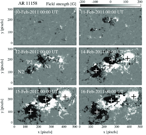
Figure 1.: SDO/HMI magnetogram of NOAA AR 11158. The flux-weighted centers of the four major polarities, P1, N1, P2, and N2, are indicated with cross signs. One pixel corresponds to 0.5 arcsec. fig:hmi

Figure fig:hmi presents the magnetic evolution of AR 11158. This AR is basically composed of two emerging bipoles, which we identify as P1–N1 and P2–N2. The first bipole [P1–N1] appeared in the southern hemisphere on 9 February, while the second pair [P2–N2] appeared on 10 February. In both bipoles, the preceding (western) polarity is positive, which agrees with the expected alignment of Hale’s polarity law (Hale et al., 1919) for Solar Cycle 24. After this, each magnetic element of both bipolar systems gradually separated from its counterpart. One of the key features of this AR is the relative motion of N1 and P2. As time progressed, the southern positive polarity P2 came closer to the northern negative polarity N1 and the magnetic gradient normal to the PIL between N1 and P2 became steeper. Then, from 13 February, P2 continuously drifted to the West and rotated around the southern edge of N1, making the PIL highly sheared and elongated. N1 and P2 shared a common penumbra, forming $\delta$-sunspots. The length of the PIL was about $30\ {\rm Mm}$ on 15 February. The counterclockwise motion of the photospheric patches N1 and P2 lasted at least until 00:00 UT, 16 February, i.e. the end of the observational data set that we analyzed. In the final stage, P2 became elongated and moved to the outmost positive polarity P1 as if P2 merged into P1. At this time, the length of the AR exceeded $150\ {\rm Mm}$.

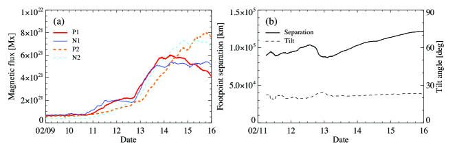
Figure 2.: (a) Total unsigned magnetic flux for each polarity. (b) Separation of the most distant polarities, P1 and N2, and the tilt angle between them. fig:ar

Figure fig:ara shows the temporal evolution of the total unsigned magnetic flux of each polarity in this AR. One may see that P1–N1 first increased its flux, particularly from 10 February, and P2–N2 increased from 11 February. Both bipoles continuously sourced their flux from a series of minor emergences. In this figure, the total flux in each bipole [P1–N1 and P2–N2] is rather balanced throughout the entire evolution. However, in the final stage, the fluxes of both inner polarities, N1 and P2, are slightly larger than their counterparts, P1 and N2, respectively. The total unsigned flux of all four patches reached $2.5\times 10^{22}\ {\rm Mx}$.

In order to quantitatively describe the geometrical evolution of this AR, we measured the flux-weighted center of each positive and negative polarity, $(x_{\pm},y_{\pm})$, which is defined as

$$\left(x_{\pm},y_{\pm}\right)=\left(\frac{\displaystyle\Sigma xB_{\pm}}{\displaystyle\Sigma B_{\pm}},\frac{\displaystyle\Sigma yB_{\pm}}{\displaystyle\Sigma B_{\pm}}\right),$$ (1)

where $B_{\pm}$ is the field strength of each pixel and $+$ ($-$) is for positive (negative) polarity. Here, only the pixels with absolute field strengths above 200 gauss are considered. Figure fig:arb shows the separation of the outmost patches P1 and N2 and their tilt angle versus time. In our definition of the tilt, the positive value indicates that it agrees with Joy’s tilt law (Hale et al., 1919); the preceding (western) polarity is on average closer to the Equator than the following (eastern) part. Therefore, Figure fig:arb indicates that the two patches gradually separated from each other up to about $115\ {\rm Mm}$, and that the tilt was almost constant with a final value of about $+23^{\circ}$, which matches Joy’s law. Here, the slight fall-off of the separation around 18:00 UT on 12 February is due to another flux increment of P1, which is also seen in Figure fig:ara.

2.2.2 Coronal Evolution

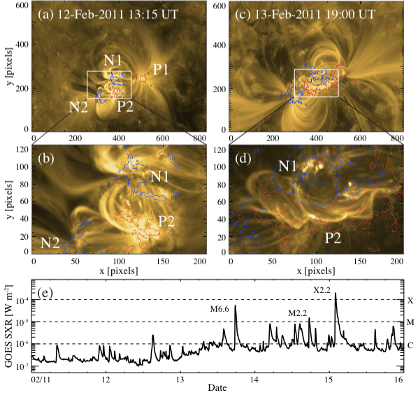
Figure 3.: Coronal evolution and flare events in AR 11158. (a) SDO/AIA 171 Å  image at 13:15 UT on 12 February 2011. One pixel corresponds to 0.6 arcsec. (b) Closeup of panel a. The field of view is shown in panel a. (c and d) Same as panels a and b but for 19:00 UT, 13 February. (e) GOES-15 soft X-ray flux of $1.0$ – $8.0$ Å  channel (five-minute cadence). fig:aia

In order to analyze the coronal structure, we also used SDO/AIA data. Figure fig:aia shows the evolution of the coronal EUV structures observed in 171 Å. As the two major bipoles, P1–N1 and P2–N2, appeared at the photosphere, corresponding coronal loops of the two bipoles also rose into the corona. One may notice that, before N1 and P2 collided with each other at 13:15 UT on 12 February as in Figures fig:aiaa and b, an arcade-like structure connecting N1 and P2 was already created, which may have been produced by the magnetic reconnection between the coronal loops of the main bipoles [P1–N1 and P2–N2]. Even when the photospheric patches N1 and P2 are still separated, the emerged magnetic fields of the two bipoles have already expanded into the corona. Between the expanding coronal loops, a current sheet is formed and eventually reconnection starts to occur.

The creation of the arcade suggests the existence of the reconnected counterpart, namely, overlying magnetic fields that connect the most distant polarities: P1 and N2. However, we did not find the clear P1–N2 loops in the 171 Å  images. This may be because the intensity at the top of the long loop is substantially weaker than that at the footpoint. If we assume that the plasma within the loop is in hydrostatic equilibrium and its temperature is about $10^{6}\ {\rm K}$ (i.e. the density scale height is $\approx 50\ {\rm Mm}$), the density at the top of the loop with a height of $50$ – $100\ {\rm Mm}$ (1 – 2 times the scale height) is several times smaller than the footpoint. Since the intensity is proportional to the square of the density, the intensity at the looptop will be at least one order of magnitude weaker than the footpoint. On 11 February, we observed that the coronal loop connecting P1–N1 suddenly expanded and became faint, which may hint at the reconnection between P1–N1 and P2–N2 and the creation of P1–N2.

At the photosphere, both inner polarities N1 and P2 continuously drifted in a counterclockwise direction with time. Here, P2 moved to the West and created a sheared PIL between N1 and P2. Figures fig:aiac and d show the corresponding coronal structure at 19:00 UT on 13 February. The arcade field N1–P2 is highly sheared, following the footpoint motions of the photospheric patches. The series of flares in this AR was observed around this sheared PIL after the PIL was formed on 13 February. Figure fig:aiae is the light curve of GOES soft X-ray flux ($1.0$ – $8.0$ Å  channel) for five days. The two strongest flares, M6.6 and X2.2, occurred at this PIL on 13 and 15 February, respectively (see, e.g., Liu et al., 2012; Sun et al., 2012). Therefore, we can conclude that the production of intense flares is strongly related to the creation of a long, sheared PIL. Note that some flares were at different locations. For example, the M2.2 event of 14 February occurred much closer to the N2 polarity, not at the central PIL.

2.3 Summary and Interpretation of the Observations

In this subsection, we summarize the observation results. NOAA AR 11158 appeared on the southern hemisphere in February 2011 as a quadrupolar region composed of two major bipoles. The eastern bipole [P1–N1] first appeared in the HMI magnetogram on 9 February and then the western pair [P2–N2] emerged on the next day. As their flux content increased, the coronal fields also became visible in the AIA images. Before the two inner polarities [N1 and P2] collided with each other to form a $\delta$-configuration, a coronal arcade connecting these two polarities was observed, which was created via magnetic reconnection between expanded coronal loops of both bipoles. However, magnetic fields arching over the entire AR were not clear, probably because the density at the looptop was much smaller than the footpoint. The continuous photospheric motion of N1 and P2 strongly sheared the PIL in the center of this AR and the coronal arcade above that. The existence of the long, sheared PIL between elongated polarities and the coronal arcade above the PIL is of great importance for producing the train of strong flares including the X2.2 and M6.6 events. The total size of this AR eventually reached more than $150\ {\rm Mm}$ and the maximum unsigned flux was $2.5\times 10^{22}\ {\rm Mx}$. We found that the fluxes of inner polarities were larger than those of outer polarities in the final stage. The centroids of the outer polarities P1 and N2 separated up to $115\ {\rm Mm}$ with a tilt angle of $+23^{\circ}$, which follows Joy’s law.

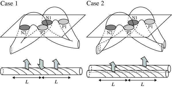
Figure 4.: (Top) Proposed concept of the flux system that forms AR 11158. Ellipses on the plane (photosphere) indicate the two major bipoles, P1–N1 and P2–N2. Lighter and darker shadows mean positive and negative polarities, respectively. Tubes above and below the photosphere show the expected flux tubes that compose this AR. Case 1 is the emergence of a single, split flux tube, while Case 2 is the emergence of two neighboring, independent tubes. (Bottom) Schematic illustration of the initial flux tubes in the numerical simulation for Cases 1 and 2. Arrows indicate the rising and sinking portions, while $L$ is the length for a field line to rotate once around the axis. fig:tube

Based on the above observation, we propose models for a global flux system that creates such a sheared PIL with a potential to produce flares. Figure fig:tube shows two possible models for AR 11158. Case 1 is the double flux emergence from a single flux tube. In this case, an isolated tube is perturbed in the convection zone and split into two, which rises to the surface as two adjacent bipoles [P1–N1 and P2–N2]. Case 2 is the emergence of two different, but neighboring, tubes. These tubes rise separately to the surface at two locations. In this case, it may be possible that the nearly simultaneous emergence of the two bipoles is triggered by the same perturbation (e.g. convective upflow). In the next section, we carry out numerical simulations to investigate which case is more realistic as a possible scenario for AR 11158.

3 Numerical Simulations sec:simulation

In order to explore the global/subsurface structure of AR 11158, particularly to study which of the magnetic systems of Figure fig:tube could produce the highly sheared, long PIL and the coronal arcade, we conducted numerical simulations of the flux tube emergence. In the observations in Section sec:observation, these features were found to be important for the production of intensive flares.

3.1 Basic Setup

The setup of the simulation is basically the same as that in Toriumi et al. (2011). Here, we solve nonlinear, time-dependent, fully compressible MHD equations. First, we set a 3D simulation box $(-120,-120,-20)\leq(x/H_{0},y/H_{0},z/H_{0})\leq(120,120,150)$, which is resolved by $256\times 256\times 256$ grid points. Here, $H_{0}$ is the normalizing unit for length. The grid spacings in the middle of the domain are $\Delta x/H_{0}=\Delta y/H_{0}=0.5$ for $(-40,-40)\leq(x/H_{0},y/H_{0})\leq(40,40)$ and $\Delta z/H_{0}=0.2$ for $-20\leq z/H_{0}\leq 20$. The spacings outside this range gradually increase. Periodic boundaries are assumed for both horizontal directions and symmetric boundaries for the vertical. We define the background stratification as the adiabatically stratified convection zone $[z/H_{0}<0]$, the cool, isothermal photosphere/chromosphere $[0\leq z/H_{0}<10]$, which we simply call the photosphere, and the hot, isothermal corona $[z/H_{0}\geq 20]$. The photosphere and the corona are smoothly connected by a transition region. Note that all of the physical values are normalized by $H_{0}=170\ {\rm km}$ for length, $C_{\rm s0}=6.8\ {\rm km\ s}^{-1}$ for velocity, $\tau_{0}=H_{0}/C_{\rm s0}=25\ {\rm seconds}$ for time, and $B_{0}=250\ {\rm gauss}$ for magnetic-field strength.

We embed initial twisted flux tubes in the convection zone. In this study, we test two cases: Case 1 is a single, split flux tube that emerges at two locations (see Case 1 of Figure fig:tube). Here, we mimic the splitting of the tube by sinking the middle part. Case 2 is the emergence of two different but neighboring flux tubes (see Case 2 of Figure fig:tube). The axial and azimuthal components of a flux tube are given as follows: for a radial distance from the axis $r=[(y-y_{\rm tube})^{2}+(z-z_{\rm tube})^{2}]^{1/2}$,

$$B_{x}(r)=B_{\rm tube}\exp{\left(-\frac{r^{2}}{R_{\rm tube}^{2}}\right)}$$ (2)

and

$$B_{\phi}(r)=qrB_{x},$$ (3)

where $(y_{\rm tube},z_{\rm tube})$ denotes the tube center, $R_{\rm tube}$ the typical radius, $q$ the twist parameter (uniform twist), and $B_{\rm tube}$ the field strength at the axis. We take $B_{\rm tube}/B_{0}=-15$, $R_{\rm tube}/H_{0}=2.5$, and $qH_{0}=0.2$ for all the tubes. Here, the axial field is directed to the negative $x$ in order to fit to the expected toroidal field in the southern hemisphere in Solar Cycle 24 and, thus, $B_{\rm tube}$ has a negative value. Moreover, these parameters mean that the twist of the tubes is right-handed, which is also favorable to the southern hemisphere (Pevtsov, Canfield, and Metcalf, 1995) and is stable against the kink instability (Linton, Longcope, and Fisher, 1996). The tubes are embedded at $(y_{\rm tube}/H_{0},z_{\rm tube}/H_{0})=(0,-10)$ for Case 1 and $(\pm 5,-10)$ for Case 2. In order to initiate their rise, we perturb the tubes by reducing densities at the initial state. The density reduction has a function of $\cos{(k_{x}x-\phi)}$, where $k_{x}=2\pi/L$ and $L=2\pi/q=10\pi H_{0}$ is the length for a field line to make one helical turn around the axis, and $\phi$ is the azimuthal angle in the cross section measured from $\hat{z}$. Note that this type of perturbation is similar to that of the helical-kink instability (e.g. Fan et al., 1998), but the present tubes are not kink-unstable, at least in the initial condition. In Case 1, we limit the density reduction to $-L\leq x\leq L$, namely, the tube is most buoyant at $x=\pm L/2$. In Case 2, the reduction is limited to $-L\leq x\leq 0$ for a tube in the negative $y$ ($y_{\rm tube}/H_{0}=-5$) and to $0\leq x\leq L$ for a tube in the positive $y$ ($y_{\rm tube}/H_{0}=5$). The bottom panels of Figure fig:tube illustrate the initial perturbations with arrows.

We also adopt anomalous resistivity only over the range of $-15\leq x/H_{0}\leq 15$ and $-10\leq y/H_{0}\leq 10$ to trigger the magnetic reconnection in the center of the computational domain. The resistivity will be switched on when the current density normalized by the plasma density exceeds the threshold, and it is a positive function of the normalized current. This promotes the reconnection at the location where the magnetic fields are anti-parallel and the density is lower (e.g. in the corona). Outside the central domain ($|x|/H_{0}>15$, $|y|/H_{0}>10$), the resistivity is always set to zero.

3.2 Results

3.2.1 Photospheric Evolution

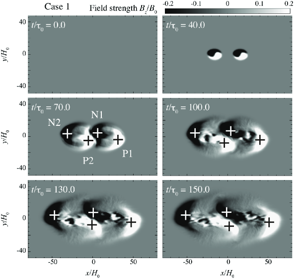
Figure 5.: Temporal evolution of the vertical fields $[B_{z}/B_{0}]$ measured at the surface $[z/H_{0}=0]$ (magnetogram) of the simulation Case 1. The flux-weighted centers of the four major polarities, P1, N1, P2, and N2, are indicated with crosses. fig:case1

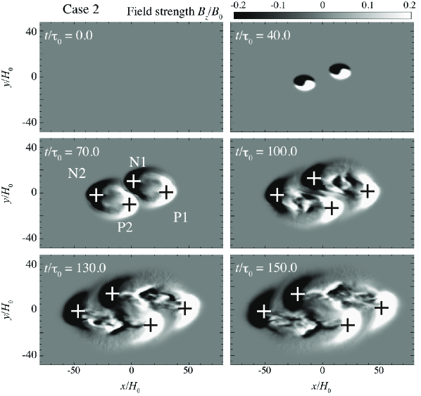
Figure 6.: Temporal evolution of the vertical fields $[B_{z}/B_{0}]$ measured at the surface $[z/H_{0}=0]$ (magnetogram) of the simulation Case 2. The flux-weighted centers of the four major polarities, P1, N1, P2, and N2, are indicated with crosses. fig:case2

Figures fig:case1 and fig:case2 show the temporal evolution of the vertical magnetic fields $[B_{z}/B_{0}]$ measured at the photosphere $[z/H_{0}=0]$ for Cases 1 and 2, respectively. In both cases, the flux appeared at the surface at $t/\tau_{0}=32$ as two pairs of positive and negative polarities, which are named P1–N1 and P2–N2 (from positive $x$). As the pair of $\Omega$-shaped loops rose into the atmosphere, each polarity of the two bipoles separated away from its counterpart.

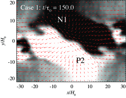
Figure 7.: Vertical and horizontal magnetic fields of Case 1 at $z/H_{0}=0$ at $t/\tau_{0}=150$. The grayscale shows the vertical fields, which saturates at $B_{z}/B_{0}=\pm 0.1$, and the red arrows indicate the horizontal fields. fig:pil

In Case 1 in Figure fig:case1, N1 and P2 approached each other at around $t/\tau_{0}=70$ and created a PIL between them. In this simulation, the two emerging bipoles belong to the same original flux tube, and thus the two inner footpoints [N1 and P2] moved to the middle of the original tube [$x/H_{0}=0$: the sinking point]. Therefore, a clear PIL was built in the middle of this quadrupolar region. Figure fig:pil shows the vertical and horizontal fields of Case 1 at the surface at $t/\tau_{0}=150$. One may see that the horizontal field on the PIL is highly sheared and is mostly parallel to the PIL, due to the elongations of N1 and P2. Also, the clustering of N1 and P2 is strongly reminiscent of the formation of $\delta$-sunspots.

Contrary to Case 1, the two inner polarities of Case 2, as shown in Figure fig:case2, did not show any significant interaction. At $t/\tau_{0}=70$, N1 and P2 approached each other at the middle of the region. However, they just passed by at $t/\tau_{0}=100$ without forming a clear PIL in between. This is because the two emerging loops originate from the two different flux tubes. The photospheric footpoints of these loops just trace the axes of their original tubes, which align parallel to each other in the $x$-direction and never cross in the convection zone. Therefore, N1 and P2 continued their migrations even after they encountered at the center of the region. Finally, at $t/\tau_{0}=150$, there were four isolated polarities with no elongated PIL in the magnetogram.

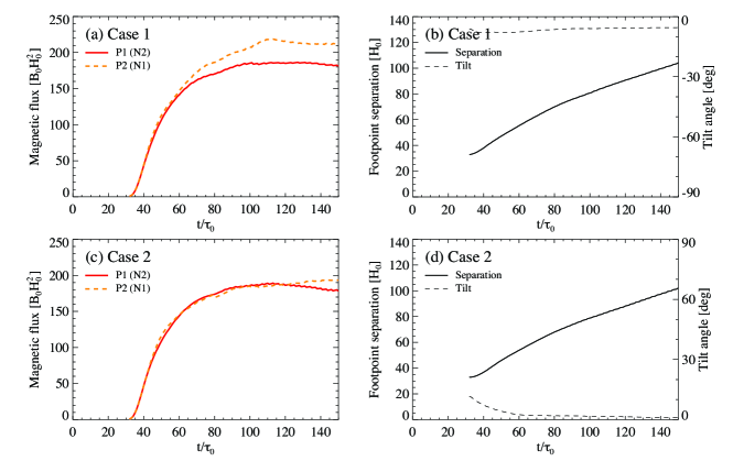
Figure 8.: (a) Total unsigned flux of P1 and P2 in the simulation Case 1. The unsigned flux of N1 and N2 is the same as that of P2 and P1, respectively, due to the symmetry of the simulation. (b) Separation between most distant polarities P1 and N2 of Case 1 and their tilt angle. (c) The same as panel a but for Case 2. (d) The same as panel b but for Case 2. fig:sim

Figure fig:sima shows total unsigned fluxes of P1 (N2) and P2 (N1) of Case 1. Note that, because of the symmetry of the simulation, the unsigned flux of N1 and N2 is just the same as P2 and P1, respectively. From this figure, we can see that there is a flux imbalance within each bipole [P1–N1 and P2–N2]. Here, the flux of the inner polarity [P2 and N1] is larger than that of its counterpart. This discrepancy can be explained by the following discussion. Some low-lying fields may undulate around the photosphere and penetrate the surface at several sites. Such serpentine field lines were found in the previous simulations (e.g. Toriumi et al., 2011). If field lines of inner polarities are more undulated as a result of the collision, the total flux of these polarities may become larger, which brings the flux imbalance between inner and outer polarities. Figure fig:simc shows that, in Case 2, the flux imbalance within each bipole is less obvious than that in Case 1. This may be because minor interactions of the inner polarities in Case 2 causes less undulation of the field lines.

The separations of outer polarities P1 and N2 of Cases 1 and 2 and their tilt angles are shown in Figures fig:simb and d, respectively. In both cases, the size of the AR continuously increased with time. At $t/\tau_{0}=150$, the separations were about $100H_{0}=17\ {\rm Mm}$. The tilt in Case 1 was almost constant and was about $-5^{\circ}$ from the $x$-axis, while, in Case 2, the tilt gradually decreased to $+1^{\circ}$. Note that our simulation models ignored the tilt produced by the Coriolis force while the flux rises through the convection zone (D’Silva and Choudhuri, 1993). The tilt here, or, the deviation from the $x$-axis, is simply caused by the twist and the relative positions of the original flux tubes.

3.2.2 Coronal Evolution

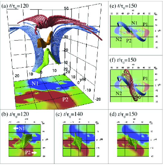
Figure 9.: Magnetic reconnection of the simulation Case 1. (a) Reconnection and the corresponding fields in the center of the simulation domain $(-20,-20)\leq(x/H_{0},y/H_{0})\leq(20,20)$ at the time $t/\tau_{0}=120$. Field lines of the two emerging bipoles (blue) reconnect and form a low-lying arcade (green) and post-reconnection fields (red). The current sheet is shown by the isosurface (orange), which is plotted over $-5\leq x/H_{0}\leq 5$, $-5\leq y/H_{0}\leq 5$, and $z/H_{0}\geq 26$. Reconnection occurs at $z/H_{0}\approx 26$. Photospheric vertical field $B_{z}/B_{0}$ is plotted at the bottom, whose color scale saturates at $0.2$ (red) and $-0.2$ (blue). (b – d) Evolution of the arcade field (green) from $t/\tau_{0}=120$ to 150. Photospheric motions of N1 and P2 are indicated with arrows in panel (b). (e and f) Top view of the field lines without and with the post-reconnection fields (red) at $t/\tau_{0}=150$. fig:bvct

In this section, we show the magnetic reconnection between the coronal fields and its evolution. Figure fig:bvcta is the closeup of the reconnection site of Case 1 for $(-20,-20)\leq(x/H_{0},y/H_{0})\leq(20,20)$ at time $t/\tau_{0}=120$. Here, the field lines of two emerging bipoles P1–N1 and P2–N2 came close to each other, and a current sheet was formed in between. Magnetic reconnection was triggered in this current sheet because of the anomalous resistivity applied to the center of the domain. As a result, a coronal arcade was produced above the photospheric PIL. Figures fig:bvctb – d show the temporal evolution of the arcade field from $t/\tau_{0}=120$ to $150$. Following the counterclockwise motion of the photospheric patches N1 and P2, the coronal arcade above the PIL was also sheared and rotated in the counterclockwise direction. At higher altitudes, another flux system was created by magnetic reconnection (post-reconnection fields). This flux was ejected from the reconnection site with an upflow of the order of the local Alfvén speed ($2$ – $6C_{s0}$). Figures fig:bvcte and f show the connectivity of the large-scale fields in the final state at $t/\tau_{0}=150$. From these figures, one can see that the emerging loops connect the two photospheric polarities of each bipole, while the post-reconnection fields link the most distant elements.

The coronal structure of simulation Case 2 is similar to that of Case 1: Both, the coronal arcade [N1–P2] and the post-reconnection fields [P1–N2] are formed by magnetic reconnection of the two emerging loops [P1–N1 and P2–N2]. However, since the photospheric patches N1 and P2 in Case 2 move away from each other very quickly and without profound interaction (see Figure fig:case2), the apparent rotational motion of the coronal arcade occurs on a much shorter time scale than that in Case 1.

3.3 Summary of the Simulations

In this section, we carried out two types of flux emergence simulation. The initial conditions were based on the proposed models of AR 11158. The first case was the emergence of a single flux tube that emerges in two portions, while, in the second case, we involved the emergence of two parallel tubes. We observed the double bipolar emergence in both cases. However, the creation of a highly sheared, elongated PIL between N1 and P2 in the center of the region was found only in Case 1. Here, in Case 1, the common subsurface root between the two emerging bipoles led to the assembly of the inner polarities, producing a packed cluster with a magnetic configuration resembling $\delta$-sunspots. The significant interaction between the two inner polarities results in the flux imbalance within each bipole. On the other hand, in Case 2, the interaction between the inner footpoints of the two horizontal tubes was not clear. These polarities just passed by each other without forming a long sheared PIL, which may be reflected in the more balanced flux within each bipole.

As time progressed, the two expanded coronal fields came close to each other and, due to the resistivity, magnetic reconnection was provoked at the center of the region. Reconnection occurred in both simulations. The emerging loops of both bipoles built a current sheet in between and reconnection proceeded to create the low-lying arcade connecting the inner polarities and post-reconnection fields joining the outmost polarities. We also observed the rotation of coronal arcade [N1–P2] in both simulations, along with the counterclockwise shearing of the photospheric patches.

4 Comparison between Observations and Simulations sec:comparison

In this article, we first analyzed the observations of NOAA AR 11158 obtained by SDO/HMI and AIA to study the evolution of this AR. The key features that we found in AR 11158 were i) the long sheared PIL between the elongated magnetic elements of opposite polarity, N1 and P2, that formed $\delta$-sunspots in the middle of the region and ii) the sheared coronal arcade above this PIL created by magnetic reconnection between $\Omega$-loops of two major bipoles. The strong flares were repeatedly produced at this PIL. Based on the observations, we proposed two scenarios for the creation of AR 11158: Case 1 is the emergence of a single split tube that emerges at two portions, while Case 2 is the emergence of two different neighboring tubes.

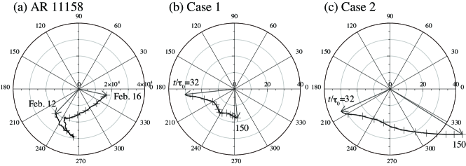
Figure 10.: Relative motion of the photospheric polarities N1 and P2 for (a) AR 11158, (b) simulation Case 1, and (c) Case 2. The center of each diagram indicates the position of N1 and the horizontal axis is parallel to the $x$-axis. (a) The plot is from 00:00 UT of 12 February 2011, to 00:00 UT, 16 February. The crosses are plotted every 12 hours and the unit for length is $1\ {\rm km}$. (b and c) The plot is from $t/\tau_{0}=32$ to 150. The crosses are plotted every $10\tau_{0}$ and the unit for length is $H_{0}=170\ {\rm km}$. fig:n1p2

Then, we conducted flux-emergence simulations of this two cases to model AR 11158. As a result, Case 1 clearly revealed a long, sheared PIL and adjacent elongated polarities N1 and P2, which is well in line with the observational results of AR 11158. However, in Case 2, these polarities just passed by each other and never built a clear PIL, which deviates from the observation. This discrepancy can easily be seen in the diagrams of Figure fig:n1p2. Here, we plot the temporal evolution of the direction and distance from the centroid of N1 to that of P2, i.e. the vector from N1 to P2. The center of the plot corresponds to the position of N1. This diagram was previously introduced by Poisson et al. (2013): see Section sec:discussion. In AR 11158, P2 continuously drifts along the southern edge of N1 from East to West in the counterclockwise direction. Here, the distance between N1 and P2 continuously decreases as the shear becomes stronger. Note that this shrinking of the vector is not caused by the change of viewing angle associated with the solar rotation, since we applied Postel’s projection to the tracked HMI magnetogram. Between the two simulation results, only Case 1 shows a similar rotating and shrinking behavior. During its anticlockwise rotation, P2 gradually gets closer to N1, creating a steep PIL. The difference between Figures fig:n1p2a and b is mainly due to the assumptions in the simulation (small numerical domain, neglected Coriolis force, etc.). For example, the separation and the tilt of P1–N2 are $115\ {\rm Mm}$ and $+23^{\circ}$ in AR 11158, while those values are $100H_{0}=17\ {\rm Mm}$ and $-5^{\circ}$ in simulation Case 1. Thus, magnifying Figure fig:n1p2b 6.8 times and rotating it $+28^{\circ}$ to match Figure fig:n1p2a, one may find clearer consistency between the two figures. However, in Case 2 in Figure fig:n1p2c, P2 approaches N1 only in the initial phase. The two polarities simply fly by and the distance becomes larger at a constant pace, which is opposite to the observed behavior of AR 11158.

Regarding the flux evolution in the photosphere, an imbalance between inner and outer polarities was observed both in AR 11158 and in the simulations. The fluxes of inner polarities were larger than those of outer polarities in the final stage. At least for the simulation, the excess of the inner flux can be explained by the fluctuation of the field lines around the surface, possibly due to the collision between the two polarities.

In both simulation cases, we found magnetic reconnection and the creation of the arcade field lying over the central PIL. The arcade structure becomes sheared following the motion of the photospheric patches. Although we did not find clear post-reconnection fields in the AIA images, which are expected to connect the most distant polarities P1 and N2, the numerical results suggest the existence of such magnetic fields.

From the above comparison, we conclude here that the flare-productive quadrupolar AR 11158 is, between the two cases, more likely to be composed of a single flux tube than two independent tubes. The single tube is severely perturbed and separated into two in the convection zone. Then, these two portions appear at the photosphere as two major bipoles. Since the bipoles share a common root beneath the surface, they recover their original configuration while the entire flux system is expanding into the corona, where the gas pressure is less dominant. Thus the inner two polarities show a strong gathering and build a highly sheared PIL. The coronal arcade is also sheared in that process, which results in the series of intense flares including X- and M-class events. If this AR were composed of two entirely separate magnetic bundles, the inner polarities cannot create such a sheared PIL, although the coronal arcade above the PIL might be built through the magnetic reconnection between coronal loops.

5 Discussion sec:discussion

As we discussed in the previous section, the SDO observations and the flux-emergence simulations suggest that, between the two possible scenarios of Figure fig:tube, the flare-productive quadrupolar AR 11158 is more likely to be made from a single subsurface flux tube. That is, the two emerging bipoles at the photosphere share a single large-scale structure in the deep convection zone. In the process of flux emergence, they recover their original shape by releasing the magnetic free energy stored within the sheared coronal arcade in the form of solar flares.

Poisson et al. (2013) observed the photospheric and coronal evolution of AR 10314. This flare-productive quadrupolar AR is very similar to AR 11158 in many aspects. Their interpretation was that AR 10314 is also created by a single flux system. Although they thought of a rising $\Omega$-loop whose top is curled downward (see Figure 7 of Poisson et al., 2013), the basic concept that the single flux system emerges at two locations is in line with our study. They argued that the packed inner polarities in the central AR would not be created by independent flux tubes. Our simulation Case 2 has revealed that their prediction is indeed true. Chintzoglou and Zhang (2013) analyzed AR 11158 and argued that this AR originates from a single flux tube deformed in the convection zone, based on the vertical stacking of the sequential HMI magnetograms (see Figure 2 of Chintzoglou and Zhang, 2013). Their concept is basically consistent with our conclusion, i.e. Case 1.

In the numerical simulations, the initial depth of the flux tubes was assumed to be $z_{\rm tube}=-10H_{0}=-1.7\ {\rm Mm}$. However, it is likely that the magnetic fields that build ARs are transported from much deeper in the convection zone. Also, in the simulations, the final separation of two outer polarities reached $100H_{0}=17\ {\rm Mm}$, which is one order of magnitude smaller than the $115\ {\rm Mm}$ observed in AR 11158. Toriumi and Yokoyama (2012; 2013) may give us a suggestion for the situation when we expand the simulation box. They found that, even when the initial flux tube is located at $-20\ {\rm Mm}$, i.e. ten times deeper than the present simulations, the flux tube indeed reaches the surface to form an AR as long as it has enough field strength, total flux, and twist. Therefore, we can expect that the simulation results may hold, at least to the depth of $20\ {\rm Mm}$.

In the simulations of this study, we did not find flare eruptions. The main reason is that a flux rope is not created after the coronal arcade is built through the magnetic reconnection between the emerging loops (see Figure fig:bvct). According to Kusano et al. (2012), in order to create a flux rope from a sheared arcade, a small-scale flare-triggering magnetic field is required, which initiates the reconnection between the coronal arcades and successfully produces flaring activity. In their simulation, the small-scale field that triggers the flare is the result of an emerging flux injected from the bottom boundary, of which the origin has not been addressed in their work. In our calculation, however, such small-scale features are not resolved. Also, according to the observation of the M6.6-class event in AR 11158 by Toriumi et al. (2013b), the formation of such a small trigger seems to be coupled with local convection. Bamba et al. (2013) analyzed the flare triggers in many more flaring events. Since our calculation does not include thermal convection, it may be difficult to create a triggering field. Therefore, in our simulation, the flux rope is not formed through the reconnection between the coronal arcades, resulting in no flare eruptions.

Here, we comment on the previous simulations of the flux-tube emergence similar to our cases. Magara (2007) simulated emergence of a single flux tube that rises at three portions. The concept looks similar to our Case 1. However, the aim of his simulation was to investigate the formation of a solar prominence. Multiple emergence from a single flux system and reconnection among these emerging loops can be found in a series of resistive-emergence simulations (Isobe, Tripathi, and Archontis, 2007; Archontis and Hood, 2009). The concept of the present Case 2, i.e. the interaction between two neighboring flux tubes in the atmosphere, is seen in Archontis, Hood, and Brady (2007), although their simulation was in 2D. Gontikakis, Archontis, and Tsinganos (2009) simulated the 3D emergence of a toroidal flux tube, not a horizontal tube, and its reconnection with a preexisting flux. They found that a slingshot reconnection produces an upward jet eruption (Archontis, Tsinganos, and Gontikakis, 2010). In our simulations, we also observed a similar upflow from the reconnection site. Archontis, Hood, and Tsinganos (2013) simulated the emergence of a weakly twisted horizontal tube and found an eruptive interaction between the two expanding lobes, which seems to be similar to our Case 1. The main difference from our work is that they calculated the emergence initially at a single location. After the flux appears at the surface, however, it rises further at two neighboring places, resulting in the dynamical interaction between the two lobes. Contrary to this, in our simulation Case 1 the initial emergence occurs at two places and thus two expanding lobes are built, which reconnect to form the coronal arcade. Another interesting result interaction between the loops in Case 1 is that $\delta$-sunspots are created from a kink-stable flux tube (see, e.g., Matsumoto et al., 1998; Fan et al., 1998). Interaction of the flux tubes within the convection zone has also been studied in detail (e.g. Fan, Zweibel, and Lantz, 1998; Linton, Dahlburg, and Antiochos, 2001; Murray and Hood, 2007). In our Case 2, there was no major interaction between the two tubes in the convection zone, since they were initially aligned in a parallel manner, and they did not expand much before they reached the photosphere. However, if we start the simulation from the deeper convection zone, or, if we consider a more complex alignment of the initial tubes, we need to take into account the tubes’ interaction beneath the surface.

6 Conclusion sec:conclusion

In this study, we compared the SDO/HMI and AIA observations of NOAA AR 11158 with the numerical simulations of the flux tube emergence, aiming to study the formation of this flare-productive AR. AR 11158, basically composed of two emerging bipoles, is one of the most flare-productive ARs in Solar Cycle 24. SDO’s continuous observation of the full solar disk at multiple wavelengths allows us to investigate the photospheric and coronal evolution of this AR from the first minutes to the moments of strong flares. The key features of this AR that we found are i) the long sheared PIL between the elongated magnetic elements of opposite polarity that produced a $\delta$-configuration in the central region and ii) the sheared coronal arcade above the PIL created by magnetic reconnection between $\Omega$-shaped loops of two major bipoles. Based on the SDO observations, we inferred two possible scenarios for the formation of AR 11158: emergence of a single split tube versus two different tubes. According to the numerical simulations, AR 11158 is more likely to be made by a single flux tube than two tubes. The single tube is severely deformed and split in two while in the convection zone. The two major bipoles at the photosphere, which share the common subsurface structure, recover their original shape during flux emergence by releasing magnetic free energy within the sheared coronal arcade in the form of solar flares including X- and M-class events.

Our study suggests that a solar flare in an AR naturally reflects the large-scale magnetic structure beneath the surface. From this point of view, flares can be thought as a process to relax magnetic shear produced by a helical and/or deformed emerging flux from the solar interior. However, we cannot observe the subsurface structure of flare-productive ARs from direct optical observations. Helioseismic detection of the emerging subsurface flux (e.g. Ilonidis, Zhao, and Kosovichev, 2011; Toriumi et al., 2013a) may improve our understanding of the nature of such ARs. Regarding the numerical simulations, neither case reproduced flare reconnection, since the evolution of the flare trigger, which may be coupled with thermal convection, was beyond the scope of the simulation code. Also, the origin of the perturbation that splits the emerging flux in two, which was mimicked by the sinking of the tube, remained unclear. These topics will be addressed in future investigations.

Acknowledgments

The authors thank K. Hayashi (Stanford University) for providing HMI data and P. Démoulin (Paris Observatory) for fruitful discussions. The authors are grateful to the anonymous referee for improving the manuscript and the SDO team for distributing HMI and AIA data. Numerical computations were carried out on Cray XC30 at the Center for Computational Astrophysics, National Astronomical Observatory of Japan. ST is supported by Grant-in-Aid for JSPS Fellows. This work was supported by a Grants-in-Aid for Scientific Research (B) “Understanding and Prediction of Triggering Solar Flares” (23340045, Head Investigator: K. Kusano) from the Ministry of Education, Science, Sports, Technology, and Culture of Japan.

References

- Archontis and Hood (2009) Archontis, V., Hood, A.W.: 2009, Formation of Ellerman bombs due to 3D flux emergence. A&A 508, 1469 – 1483. http://dx.doi.org/10.1051/0004-6361/200912455. http://ads.nao.ac.jp/abs/2009A%26A…508.1469A.
- Archontis, Hood, and Brady (2007) Archontis, V., Hood, A.W., Brady, C.: 2007, Emergence and interaction of twisted flux tubes in the Sun. A&A 466, 367 – 376. http://dx.doi.org/10.1051/0004-6361:20066508. http://ads.nao.ac.jp/abs/2007A%26A…466..367A.
- Archontis, Hood, and Tsinganos (2013) Archontis, V., Hood, A.W., Tsinganos, K.: 2013, The Emergence of Weakly Twisted Magnetic Fields in the Sun. ApJ 778, 42. http://dx.doi.org/10.1088/0004-637X/778/1/42. http://ads.nao.ac.jp/abs/2013ApJ…778…42A.
- Archontis, Tsinganos, and Gontikakis (2010) Archontis, V., Tsinganos, K., Gontikakis, C.: 2010, Recurrent solar jets in active regions. A&A 512, L2. http://dx.doi.org/10.1051/0004-6361/200913752. http://ads.nao.ac.jp/abs/2010A%26A…512L…2A.
- Bamba et al. (2013) Bamba, Y., Kusano, K., Yamamoto, T.T., Okamoto, T.J.: 2013, Study on the Triggering Process of Solar Flares Based on Hinode/SOT Observations. ApJ 778, 48. http://dx.doi.org/10.1088/0004-637X/778/1/48. http://ads.nao.ac.jp/abs/2013ApJ…778…48B.
- Chintzoglou and Zhang (2013) Chintzoglou, G., Zhang, J.: 2013, Reconstructing the Subsurface Three-dimensional Magnetic Structure of a Solar Active Region Using SDO/HMI Observations. ApJ 764, L3. http://dx.doi.org/10.1088/2041-8205/764/1/L3. http://ads.nao.ac.jp/abs/2013ApJ…764L…3C.
- D’Silva and Choudhuri (1993) D’Silva, S., Choudhuri, A.R.: 1993, A theoretical model for tilts of bipolar magnetic regions. A&A 272, 621. http://ads.nao.ac.jp/abs/1993A%26A…272..621D.
- Fan (2009) Fan, Y.: 2009, Magnetic Fields in the Solar Convection Zone. Living Reviews in Solar Physics 6, 4. http://dx.doi.org/10.12942/lrsp-2009-4. http://ads.nao.ac.jp/abs/2009LRSP….6….4F.
- Fan, Zweibel, and Lantz (1998) Fan, Y., Zweibel, E.G., Lantz, S.R.: 1998, Two-dimensional Simulations of Buoyantly Rising, Interacting Magnetic Flux Tubes. ApJ 493, 480. http://dx.doi.org/10.1086/305122. http://ads.nao.ac.jp/abs/1998ApJ…493..480F.
- Fan et al. (1998) Fan, Y., Zweibel, E.G., Linton, M.G., Fisher, G.H.: 1998, The Rise of Kink-Unstable Magnetic Flux Tubes in the Solar Convection Zone. ApJ 505, L59. http://dx.doi.org/10.1086/311597. http://ads.nao.ac.jp/abs/1998ApJ…505L..59F.
- Gontikakis, Archontis, and Tsinganos (2009) Gontikakis, C., Archontis, V., Tsinganos, K.: 2009, Observations and 3D MHD simulations of a solar active region jet. A&A 506, L45 – L48. http://dx.doi.org/10.1051/0004-6361/200913026. http://ads.nao.ac.jp/abs/2009A%26A…506L..45G.
- Hagyard et al. (1984) Hagyard, M.J., Teuber, D., West, E.A., Smith, J.B.: 1984, A quantitative study relating observed shear in photospheric magnetic fields to repeated flaring. Sol. Phys. 91, 115 – 126. http://dx.doi.org/10.1007/BF00213618. http://ads.nao.ac.jp/abs/1984SoPh…91..115H.
- Hale et al. (1919) Hale, G.E., Ellerman, F., Nicholson, S.B., Joy, A.H.: 1919, The Magnetic Polarity of Sun-Spots. ApJ 49, 153. http://dx.doi.org/10.1086/142452. http://ads.nao.ac.jp/abs/1919ApJ….49..153H.
- Ilonidis, Zhao, and Kosovichev (2011) Ilonidis, S., Zhao, J., Kosovichev, A.: 2011, Detection of Emerging Sunspot Regions in the Solar Interior. Science 333, 993. http://dx.doi.org/10.1126/science.1206253. http://ads.nao.ac.jp/abs/2011Sci…333..993I.
- Isobe, Tripathi, and Archontis (2007) Isobe, H., Tripathi, D., Archontis, V.: 2007, Ellerman Bombs and Jets Associated with Resistive Flux Emergence. ApJ 657, L53 – L56. http://dx.doi.org/10.1086/512969. http://ads.nao.ac.jp/abs/2007ApJ…657L..53I.
- Kusano et al. (2012) Kusano, K., Bamba, Y., Yamamoto, T.T., Iida, Y., Toriumi, S., Asai, A.: 2012, Magnetic Field Structures Triggering Solar Flares and Coronal Mass Ejections. ApJ 760, 31. http://dx.doi.org/10.1088/0004-637X/760/1/31. http://ads.nao.ac.jp/abs/2012ApJ…760…31K.
- Lemen et al. (2012) Lemen, J.R., Title, A.M., Akin, D.J., Boerner, P.F., Chou, C., Drake, J.F., Duncan, D.W., Edwards, C.G., Friedlaender, F.M., Heyman, G.F., Hurlburt, N.E., Katz, N.L., Kushner, G.D., Levay, M., Lindgren, R.W., Mathur, D.P., McFeaters, E.L., Mitchell, S., Rehse, R.A., Schrijver, C.J., Springer, L.A., Stern, R.A., Tarbell, T.D., Wuelser, J.-P., Wolfson, C.J., Yanari, C., Bookbinder, J.A., Cheimets, P.N., Caldwell, D., Deluca, E.E., Gates, R., Golub, L., Park, S., Podgorski, W.A., Bush, R.I., Scherrer, P.H., Gummin, M.A., Smith, P., Auker, G., Jerram, P., Pool, P., Soufli, R., Windt, D.L., Beardsley, S., Clapp, M., Lang, J., Waltham, N.: 2012, The Atmospheric Imaging Assembly (AIA) on the Solar Dynamics Observatory (SDO). Sol. Phys. 275, 17 – 40. http://dx.doi.org/10.1007/s11207-011-9776-8. http://ads.nao.ac.jp/abs/2012SoPh..275…17L.
- Linton, Dahlburg, and Antiochos (2001) Linton, M.G., Dahlburg, R.B., Antiochos, S.K.: 2001, Reconnection of Twisted Flux Tubes as a Function of Contact Angle. ApJ 553, 905 – 921. http://dx.doi.org/10.1086/320974. http://ads.nao.ac.jp/abs/2001ApJ…553..905L.
- Linton, Longcope, and Fisher (1996) Linton, M.G., Longcope, D.W., Fisher, G.H.: 1996, The Helical Kink Instability of Isolated, Twisted Magnetic Flux Tubes. ApJ 469, 954. http://dx.doi.org/10.1086/177842. http://ads.nao.ac.jp/abs/1996ApJ…469..954L.
- Liu et al. (2012) Liu, C., Deng, N., Liu, R., Lee, J., Wiegelmann, T., Jing, J., Xu, Y., Wang, S., Wang, H.: 2012, Rapid Changes of Photospheric Magnetic Field after Tether-cutting Reconnection and Magnetic Implosion. ApJ 745, L4. http://dx.doi.org/10.1088/2041-8205/745/1/L4. http://ads.nao.ac.jp/abs/2012ApJ…745L…4L.
- Magara (2007) Magara, T.: 2007, A Possible Structure of the Magnetic Field in Solar Filaments Obtained by Flux Emergence. PASJ 59, L51. http://ads.nao.ac.jp/abs/2007PASJ…59L..51M.
- Matsumoto et al. (1998) Matsumoto, R., Tajima, T., Chou, W., Okubo, A., Shibata, K.: 1998, Formation of a Kinked Alignment of Solar Active Regions. ApJ 493, L43. http://dx.doi.org/10.1086/311116. http://ads.nao.ac.jp/abs/1998ApJ…493L..43M.
- Murray and Hood (2007) Murray, M.J., Hood, A.W.: 2007, Simple emergence structures from complex magnetic fields. A&A 470, 709 – 719. http://dx.doi.org/10.1051/0004-6361:20077251. http://ads.nao.ac.jp/abs/2007A%26A…470..709M.
- Pesnell, Thompson, and Chamberlin (2012) Pesnell, W.D., Thompson, B.J., Chamberlin, P.C.: 2012, The Solar Dynamics Observatory (SDO). Sol. Phys. 275, 3 – 15. http://dx.doi.org/10.1007/s11207-011-9841-3. http://ads.nao.ac.jp/abs/2012SoPh..275….3P.
- Pevtsov, Canfield, and Metcalf (1995) Pevtsov, A.A., Canfield, R.C., Metcalf, T.R.: 1995, Latitudinal variation of helicity of photospheric magnetic fields. ApJ 440, L109 – L112. http://dx.doi.org/10.1086/187773. http://ads.nao.ac.jp/abs/1995ApJ…440L.109P.
- Poisson et al. (2013) Poisson, M., López Fuentes, M., Mandrini, C.H., Démoulin, P., Pariat, E.: 2013, Study of magnetic flux emergence and related activity in active region NOAA 10314. Advances in Space Research 51, 1834 – 1841. http://dx.doi.org/10.1016/j.asr.2012.03.010. http://ads.nao.ac.jp/abs/2013AdSpR..51.1834P.
- Sammis, Tang, and Zirin (2000) Sammis, I., Tang, F., Zirin, H.: 2000, The Dependence of Large Flare Occurrence on the Magnetic Structure of Sunspots. ApJ 540, 583 – 587. http://dx.doi.org/10.1086/309303. http://ads.nao.ac.jp/abs/2000ApJ…540..583S.
- Scherrer et al. (2012) Scherrer, P.H., Schou, J., Bush, R.I., Kosovichev, A.G., Bogart, R.S., Hoeksema, J.T., Liu, Y., Duvall, T.L., Zhao, J., Title, A.M., Schrijver, C.J., Tarbell, T.D., Tomczyk, S.: 2012, The Helioseismic and Magnetic Imager (HMI) Investigation for the Solar Dynamics Observatory (SDO). Sol. Phys. 275, 207 – 227. http://dx.doi.org/10.1007/s11207-011-9834-2. http://ads.nao.ac.jp/abs/2012SoPh..275..207S.
- Schou et al. (2012) Schou, J., Scherrer, P.H., Bush, R.I., Wachter, R., Couvidat, S., Rabello-Soares, M.C., Bogart, R.S., Hoeksema, J.T., Liu, Y., Duvall, T.L., Akin, D.J., Allard, B.A., Miles, J.W., Rairden, R., Shine, R.A., Tarbell, T.D., Title, A.M., Wolfson, C.J., Elmore, D.F., Norton, A.A., Tomczyk, S.: 2012, Design and Ground Calibration of the Helioseismic and Magnetic Imager (HMI) Instrument on the Solar Dynamics Observatory (SDO). Sol. Phys. 275, 229 – 259. http://dx.doi.org/10.1007/s11207-011-9842-2. http://ads.nao.ac.jp/abs/2012SoPh..275..229S.
- Schrijver et al. (2011) Schrijver, C.J., Aulanier, G., Title, A.M., Pariat, E., Delannée, C.: 2011, The 2011 February 15 X2 Flare, Ribbons, Coronal Front, and Mass Ejection: Interpreting the Three-dimensional Views from the Solar Dynamics Observatory and STEREO Guided by Magnetohydrodynamic Flux-rope Modeling. ApJ 738, 167. http://dx.doi.org/10.1088/0004-637X/738/2/167. http://ads.nao.ac.jp/abs/2011ApJ…738..167S.
- Shibata and Magara (2011) Shibata, K., Magara, T.: 2011, Solar Flares: Magnetohydrodynamic Processes. Living Reviews in Solar Physics 8, 6. http://dx.doi.org/10.12942/lrsp-2011-6. http://ads.nao.ac.jp/abs/2011LRSP….8….6S.
- Sun et al. (2012) Sun, X., Hoeksema, J.T., Liu, Y., Wiegelmann, T., Hayashi, K., Chen, Q., Thalmann, J.: 2012, Evolution of Magnetic Field and Energy in a Major Eruptive Active Region Based on SDO/HMI Observation. ApJ 748, 77. http://dx.doi.org/10.1088/0004-637X/748/2/77. http://ads.nao.ac.jp/abs/2012ApJ…748…77S.
- Toriumi and Yokoyama (2012) Toriumi, S., Yokoyama, T.: 2012, Large-scale 3D MHD simulation on the solar flux emergence and the small-scale dynamic features in an active region. A&A 539, A22. http://dx.doi.org/10.1051/0004-6361/201118009. 2012A%26A…539A..22T.
- Toriumi and Yokoyama (2013) Toriumi, S., Yokoyama, T.: 2013, Three-dimensional magnetohydrodynamic simulation of the solar magnetic flux emergence. Parametric study on the horizontal divergent flow. A&A 553, A55. http://dx.doi.org/10.1051/0004-6361/201321098. 2013A%26A…553A..55T.
- Toriumi et al. (2011) Toriumi, S., Miyagoshi, T., Yokoyama, T., Isobe, H., Shibata, K.: 2011, Dependence of the Magnetic Energy of Solar Active Regions on the Twist Intensity of the Initial Flux Tubes. PASJ 63, 407 – 415. http://ads.nao.ac.jp/abs/2011PASJ…63..407T.
- Toriumi et al. (2013a) Toriumi, S., Ilonidis, S., Sekii, T., Yokoyama, T.: 2013a, Probing the Shallow Convection Zone: Rising Motion of Subsurface Magnetic Fields in the Solar Active Region. ApJ 770, L11. http://dx.doi.org/10.1088/2041-8205/770/1/L11. http://ads.nao.ac.jp/abs/2013ApJ…770L..11T.
- Toriumi et al. (2013b) Toriumi, S., Iida, Y., Bamba, Y., Kusano, K., Imada, S., Inoue, S.: 2013b, The Magnetic Systems Triggering the M6.6 Class Solar Flare in NOAA Active Region 11158. ApJ 773, 128. http://dx.doi.org/10.1088/0004-637X/773/2/128. http://ads.nao.ac.jp/abs/2013ApJ…773..128T.