Theory of the Magnetic Resonance for the High-$T_{C}$ Copper-Oxide Superconductors

Abstract

The magnetic response expected from a state characterized by rotating antiferromagnetism in a neutron-scattering experiment is calculated. We predict the occurrence of a peak at the frequency of the rotation of the rotating antiferromagnetic order parameter. The doping dependence of this frequency is very similar to that of the frequency of the magnetic resonance observed in the neutron-scattering experiments for the hole-doped high-$T_{C}$ cuprates. This leads us to propose the rotating antiferromagnetism as a possible mechanism for this magnetic resonance. We conclude that while the magnitude of the rotating antiferromagnetic order parameter was previously proposed to be responsible for the pseudogap and the unusual thermodynamic and transport properties, the phase of the rotating order parameter is proposed here to be responsible for the unusual magnetic properties of the high-$T_{C}$ copper-oxide superconductors.

I Introduction

The bulk of the experimental data collected so far on the magnetic properties of the hole-doped high-$T_{C}$ cuprate superconductors can be classified using three main key features or behaviors: i) The unusual zero momentum (${\bf q}=0$) static antiferromagnetic order first discovered by Fauqué et al.fauque2006 in the hole-underdoped YBa₂Cu₃O_6+x system. Subsequently, this unusual order was also observed in the same regime for the single-layer cuprate HgBa₂CuO_4+δ.li2008 Interestingly, this order develops exactly below the doping-dependent pseudogaptimusk1998 (PG) temperature, indicating the existence of a connection between the PG and this order. ii) Second, the hour-glass magnetic spectrum shapefujita2012 in general or the magnetic resonancerossat-mignod1991 in particular, which characterizes the magnetic excitation energies as a function of momentum for the hole-doped materials. Contrary to the zero-momentum order, the hour-glass spectrum highlights clearly the importance of the usual antiferromagnetic correlations because this spectrum is centered around the antiferromagnetic momentum ${\bf Q}_{AF}=(\pi,\pi)$, where the resonance has been observed for most hole-doped high-$T_{C}$ cuprates. iii) And third, magnetic excitations were seen within the PG phase by Li et al.li2010 in the HgBa₂CuO_4+δ system. This material is also characterized by the unusual static zero-momentum antiferromagnetism.li2008 These excitations develop in the whole Brillouin zone below the PG temperature, and interestingly seem to connect with the ${\bf Q}_{AF}$ resonance observed also in this material.yu2010 This again indicates that the magnetic properties and the PG behavior observed in charge-like properties are very likely related.

Out of the sake of completeness, one must mention the spin response of isolated layers of the parent undoped compound La₂CuO₄, which are only one unit cell thick.dean2012 This response consisted of the same coherent magnetic excitations, namely magnons, which occur for the bulk order. Because long-range order cannot exist in a single layer, the magnons in a single layer need to find an explanation outside of the conventional spin-wave theory.

Consequently, a theoretical model for the high-$T_{C}$ materials must not only account for the PG and the magnetic resonance phenomena separately, but also take into account the feature in iii, which suggests that what causes the PG is perhaps responsible for the magnetic resonance as well. This model ought to account also for the magon-like response obtained for a single layer of La₂CuO₄, at least qualitatively for now. In this paper, we argue that the rotating antiferromagnetism theory (RAFT) satisfies this criterion.azzouz2003 ; azzouz2003p ; azzouz2004 ; azzouz2005 ; azzouz2010 ; azzouz2010p ; azzouz2012 ; azzouz2012p ; azzouz2013 RAFT, which was originally proposed in order to explain the PG behavior in these materials, yield results in general consistent with experimental data for angle-resolved-photoemission,azzouz2010 optical conductivity,azzouz2005 ; azzouz2012 Raman,azzouz2010 and thermodynamic properties.azzouz2003p ; azzouz2004 This theory is based on the phenomenon of the rotating antiferromagnetic (RAF) order whose order parameter is a vector magnetization with a nonzero magnitude and a time-dependent phase. This time dependence makes of the RAF order an example of hidden order in a spin-liquid state. RAFT is one among other theoretical proposals for the PG,he2011 and is based on spin antiferromagnetism contrary to the theories of circulating currentsvarma1997 ; varma2006 ; chakravarty2001 which are based on hidden orbital antiferromagnetism. Like these theories, RAFT belongs in the competition (between some sort of magnetism and superconductivity) scenario, contrary to the theory which is based on the preformed superconducting pairs scenario.emery1995 An argument in favor of a theory based on spin antiferromagnetism rather than one based on orbital antiferromagnetism is that the unusual antiferromagnetic ${\bf q}=0$ order was observed by counting spin flip events. In our opinion, the latter can only be defined for a spin $1/2$. If one assumes the conservation of the angular momentum in the scattering process, then a spin flip for the neutron has to be compensated by a spin flip in the excitation of the system, and this can occur only for the real spin of the electron (or hole); the orbital current has an integral angular momentum. If true, this argument will rule out the candidacy of any theory based on circulating currents for the explanation of the unusual ${\bf q}=0$ antiferromagnetism and the PG. We will discuss this point again later in the framework of RAFT. In the latter, the PG below $T^{*}$ is caused by the magnitude of the RAF order parameter. In the present report, we argue that the phase of this parameter is responsible for the magnetic ${\bf Q}_{AF}$ resonance observed at nonzero doping-dependent frequencies.

The time dependence of the phase of the RAF order parameter remained an issue until recently when a crude estimate was derived in the limit of localized electrons, where the effects of the kinetic energy and doping were neglected.azzouz2012p This estimate was obtained using the Heisenberg dynamics’ equation where only the onsite Coulomb repulsion of the Hubbard Hamiltonian was incorporated in the equation’s commutator, independently of the doping level. Note that RAFT is implemented using the two-dimensional Hubbard model. Even though the physical interpretation of the RAF order found within the crude treatment of Ref. azzouz2012p, remains correct, this approximation led to a doping- and momentum-independent phase. The lack of the doping dependence made the comparison with available experimental data, like those of the neutron scattering experiments, impossible. It is worth stressing that all the physical properties calculated or analyzed so far within RAFT do not depend on the phase of the RAF order parameter. Comparison of the results of such works with experimental data led to satisfactory agreement in general. azzouz2003 ; azzouz2003p ; azzouz2004 ; azzouz2005 ; azzouz2010 ; azzouz2010p ; azzouz2012 ; azzouz2012p ; azzouz2013

The time dependence of the phase of the RAF order parameter is recalculated in the present work using the total RAFT’s mean-field Hamiltonian in the Heisenberg equation. This yields an expression that takes into account the doping dependence for the rotational angular frequency $\omega_{sf}$ of this order parameter. The results obtained for $\omega_{sf}$ for different Hamiltonian parameters are discussed in connection with existing neutron scattering data.fujita2012 The shape of the spin excitations for most of the hole-doped materials is the famous hour-glass dispersion, which is characterized by an upwardly component separated at the waist of the hour glass by a doping dependent energy $E_{\rm cross}$ from a downwardly component. Below $E_{\rm cross}$, the peaks in the magnetic response occur at incommensurate momenta, but at $E_{\rm cross}$, the response’s peak occurs at the commensurate momentum $(\pi,\pi)$. The rotating magnetization in RAFT introduces an energy scale $\hbar\omega_{sf}$, which, as we argue here, is identified with $E_{\rm cross}$, and is thus related to the ${\bf Q}_{AF}\equiv(\pi,\pi)$ resonance observed in neutron scattering experiments.

The remainder of this paper is organized as follows. First, in order to estimate the contribution of the RAF order in the neutron scattering experiments, we analyze the scattering cross-section for this hidden order. Then, we calculate the time dependence of the phase of the rotating order parameter, and explain its connection with this cross-section. Afterward, we calculate the doping dependence of the frequency of rotation and discuss it in terms of the magnetic resonance energy measured experimentally. Finally, conclusions are drawn.

II Approach

II.1 Calculation of the neutron scattering cross-section for RAF order

To understand the response expected from a state with RAF order, we calculate the contribution of such an order to the cross-section starting from the well known expressionsquires

$$\frac{d^{2}\sigma}{d\Omega dE^{\prime}} \propto \sum_{\ell,\ell^{\prime}}\sum_{\alpha,\beta}(\delta_{\alpha\beta}-{\hat{q}}_{\alpha}{\hat{q}}_{\beta})e^{i{\bf q}\cdot({\bf R}_{\ell}-{\bf R}_{\ell^{\prime}})}\int dt\langle S_{\ell^{\prime}}^{\alpha}(0)S_{\ell}^{\beta}(t)\rangle e^{-i\omega t},$$ (1)

and focus on the spin-spin correlation function. ${\hat{q}}_{\alpha}$ is the $\alpha$-component of the unit vector ${\hat{\bf q}}={\bf q}/q$; ${\bf q}$ is the momentum transfer of the neutron and $\alpha=x,y,z$. In RAFT,azzouz2003

$$\langle S_{\ell}^{x}\rangle=Q_{\ell}\cos[\phi(t)],$$ (2)

$$\langle S_{\ell}^{y}\rangle=Q_{\ell}\sin[\phi(t)],$$ (3)

$$\langle S_{\ell}^{z}\rangle=0,$$ (4)

where $Q_{\ell}=e^{\pm i{\bf Q}_{AF}\cdot{\bf R}_{\ell}}Q$ is a staggered magnetization; $Q$ being its magnitude. Here, ${\bf R}_{\ell}=x_{\ell}{\hat{x}}+y_{\ell}{\hat{y}}$ designates the coordinates of site $\ell$ on a two-dimensional lattice. $\phi(t)$ is the phase of the RAF order parameter, whose time dependence will be calculated below. But first let us find out how the cross-section (1) depends on this phase or its time derivative (angular frequency). If we were to use Eqs. (4) in (1) for a static helical order with a time-independent phase $\phi$, then the cross-section would have an elastic component at zero energy $\omega=0$.squires For RAF, such an elastic contribution does not exit, but a peak at a finite frequency (energy) can be shown to exist.

In the limit $t\to\infty$, we use the same approximation that leads to the elastic contribution for ordinary magnetic orders,squires namely $\lim_{t\to\infty}\langle S_{\ell^{\prime}}^{\alpha}(0)S_{\ell}^{\beta}(t)\rangle\approx\langle S_{\ell^{\prime}}^{\alpha}(0)\rangle\langle S_{\ell}^{\beta}(t)\rangle$. Normally, for static order, the values of the expectation values appearing on the right hand side of this equality are the static values of the order parameter. Here we replace the time dependence for $\langle S_{\ell}^{\beta}(t)\rangle$ by the components of the RAF order parameter given by expressions (4). As found below, the consequences of this assumption are pretty consistent with the neutron-scattering experimental results regarding the magnetic resonance. Calculating $\langle S_{\ell^{\prime}}^{\alpha}(0)S_{\ell}^{\beta}(t)\rangle$ for $\alpha=x,\ y,\ z$ and $\beta=x,\ y,\ z$ leads to

$$Q^{2}\sum_{\ell,\ell^{\prime}}\int dte^{-i\omega t}\big{\{}\cos[\phi(t)-\phi(0)]-\frac{1}{2}({\hat{q}}_{x}^{2}+{\hat{q}}_{y}^{2})\cos[\phi(t)-\phi(0)]$$ (5)

$$-\frac{1}{2}({\hat{q}}_{x}^{2}-{\hat{q}}_{y}^{2})\cos[\phi(t)+\phi(0)]-{\hat{q}}_{x}{\hat{q}}_{y}\sin[\phi(t)+\phi(0)\big{\}}e^{i({\bf Q}_{AF}+{\bf q})\cdot({\bf R}_{\ell}-{\bf R}_{\ell^{\prime}})}.$$ (6)

Expression (6) becomes the same as in the case of a helical arrangement when $\phi(0)$ is replaced by ${\bf Q}\cdot{\bf R}_{\ell}$ and $\phi(t)$ by ${\bf Q}\cdot{\bf R}_{\ell^{\prime}}$. The vector ${\bf Q}$ is in the direction of the axis of the helix, is of magnitude $2\pi$ divided by the pitch of the helix,squires and should not be confused with the RAF order parameter $Q$, which has the physical unit of magnetization. As mentioned later on, $Q$ is calculated self-consistently using RAFT’s mean-field equations.azzouz2003 ; azzouz2003p ; azzouz2004

Next we Taylor expand $\phi(t)$ to first order in time. One gets $\phi(t)-\phi(0)\approx\omega_{sf}t$, where $\omega_{sf}$ is the rotational angular frequency of the RAF order parameter. Then, $\phi(t)+\phi(0)=\omega_{sf}t+2\phi(0)$. Because there is no reason for the initial phase $\phi(0)$ to be non random, averaging over it must yield zero for the terms in $\cos[\phi(t)+\phi(0)]$ and $\sin[\phi(t)+\phi(0)]$ in Eq. (6), which then reduces to

$$Q^{2}\sum_{\ell,\ell^{\prime}}\int dte^{-i\omega t}\big{[}1-\frac{1}{2}({\hat{q}}_{x}^{2}+{\hat{q}}_{y}^{2})\big{]}\cos(\omega_{sf}t)e^{i({\bf Q}_{AF}+{\bf q})\cdot({\bf R_{\ell}}-{\bf R}_{\ell^{\prime}})}=$$ (7)

$$N(2\pi)^{2}Q^{2}(1+{\hat{q}}_{z}^{2})\sum_{\bf G}\delta({\bf q}+{\bf Q}_{AF}+{\bf G})\big{[}\delta(\omega-\omega_{sf})+\delta(\omega+\omega_{sf})\big{]},$$ (8)

where $N$ is the number of the lattice sites, and ${\bf G}$ a reciprocal lattice vector. Expression (8) is nonzero only when the momentum transfer is ${\bf q}\equiv{\bf Q}_{AF}$ [mod. a reciprocal lattice vector], and when the neutron’s energy transfer satisfies $\omega=\pm\omega_{sf}$. The occurrence of a peak in Eq. (8) at the momentum transfer ${\bf Q}_{AF}=(\pi,\pi)$ and at a finite energy reminds us of the observed magnetic resonance in hole-doped high-$T_{C}$ cuprates.fujita2012 To push one step further the comparison of our results with the experimental data for this resonance, we calculate $\omega_{sf}$ as a function of doping and compare it with that of the resonance energy or $E_{\rm cross}$.fujita2012

II.2 Calculation of the peak frequency $\omega_{sf}$ within RAFT

In Ref. azzouz2012p, , the crude estimate $\omega_{sf}\approx U/\hbar$ was derived in the limit of localized electrons, where the effects of doping and electrons’ kinetic energy were neglected. To get this expression, only the $U$ term of the Hubbard Hamiltonian was considered in the Heisenberg equation. Tremblay,tremblay2013 however, pointed out that the frequency $\omega_{sf}$ needs be calculated using the mean-field RAFT’s Hamiltonian instead of the U-term of the Hubbard model. When calculated as such as shown below, $\omega_{sf}$ is found to show significant doping and wavevector dependence.

In order to proceed, we use the definition of the RAF order parameter $Q_{\ell}$ in RAFT, namely $Q_{\ell}=-\langle c_{\ell\uparrow}^{\alpha{\dagger}}c^{\alpha}_{\ell\downarrow}\rangle=-\frac{1}{N}\sum_{\bf k}\langle c_{{\bf k}\uparrow}^{\alpha{\dagger}}c^{\alpha}_{{\bf k}\downarrow}\rangle$, with $\ell\in$ sublattice $\alpha=A$ or $B$. For a site-independent phase, we can get this time dependence by considering the Green’s function $\langle c_{{\bf k}\uparrow}^{\alpha{\dagger}}(t)c_{{\bf k}\downarrow}^{\alpha}(0)\rangle$ with $t>0$. Physically, the time dependence of a spin flip process can be calculated via $\langle c_{{\bf k}\uparrow}^{A{\dagger}}(t)c_{{\bf k}\downarrow}^{A}(0)\rangle$ for sublattice $A$, which means that a spin-down electron is annihilated in state ${\bf k}$ at an earlier time $t=0$, then a spin-up electron is created at a later time $t>0$. To get the time dependence of $\langle c_{{\bf k}\uparrow}^{\alpha{\dagger}}(t)c_{{\bf k}\downarrow}^{\alpha}(0)\rangle$ we calculate the time dependence of $c_{{\bf k}\uparrow}^{\alpha{\dagger}}(t)$ using the Heisenberg equation with the RAFT Hamiltonian in the commutator. Note that in Ref. azzouz2012p, , the time dependence of $S^{\pm}$ was rather sought. This is one of the reasons why an accurate estimate of the frequency was not obtained.

Given the difficulty and complexity of the problem under investigation here, we restrict our analysis to the non superconducting phase. In this case, RAFT’s Hamiltonian is given byazzouz2013 ; azzouz2003 ; azzouz2003p ; azzouz2004

$$H\approx\sum_{{\bf k}\in RBZ}\Psi^{{\dagger}}_{\bf k}{\cal H}\Psi_{\bf k}+NUQ^{2}-NUn^{2},$$ (9)

where $Q=|\langle c_{\ell\downarrow}c_{\ell\uparrow}^{\dagger}\rangle|$, $n=\langle n_{i,\sigma}\rangle$ is the expectation value of the number operator, and $U$ is the onsite Coulomb repulsion energy. Due to the antiferromagnetic correlations present in the system even when no long-range order occurs well away from half-filling, the lattice is considered to be made of two sublattices $A$ and $B$. The summation runs over the magnetic or reduced Brillouin zone (RBZ). The 4-component Nambu spinor is

$$\Psi^{\dagger}=(\Psi_{{{\bf k}}1}^{\dagger},\Psi_{{{\bf k}}2}^{\dagger},\Psi_{{{\bf k}}3}^{\dagger},\Psi_{{{\bf k}}4}^{\dagger})\equiv(c^{A{\dagger}}_{{{\bf k}}\uparrow},c^{B{\dagger}}_{{{\bf k}}\uparrow},c^{A{\dagger}}_{{{\bf k}}\downarrow},c^{B{\dagger}}_{{{\bf k}}\downarrow}),$$ (10)

and the Hamiltonian matrix is

$${\cal H}=\left(\begin{array}[]{cccc}-\mu^{\prime}({\bf k})&\epsilon({\bf k})&QU&0\\ \epsilon({\bf k})&-\mu^{\prime}({\bf k})&0&-QU\\ QU&0&-\mu^{\prime}({\bf k})&\epsilon({\bf k})\\ 0&-QU&\epsilon({\bf k})&-\mu^{\prime}({\bf k})\end{array}\right).$$ (15)

The eigenenergies are $E_{\pm}({\bf k})=-\mu^{\prime}({\bf k})\pm E_{q}({\bf k})$, with $E_{q}({\bf k})=\sqrt{\epsilon^{2}({\bf k})+Q^{2}U^{2}}$, and $\mu^{\prime}=\mu-Un-4t^{\prime}\cos k_{x}\cos k_{y}$; $\mu$ being the chemical potential, and $\epsilon({\bf k})=-2t(\cos k_{x}+\cos k_{y})$. $t$, ($t^{\prime}$), is electrons’ hopping energy between first (second)-nearest neighbors. $Q$ and $n$ are calculated self-consistently using RAFT’s mean-field equations:azzouz2003

$$1 = \frac{U}{2N}\sum_{\bf k}\frac{n_{F}[E_{-}({\bf k})]-n_{F}[E_{+}({\bf k})]}{E_{q}({\bf k})},$$ (16)

$$n = \frac{1}{2N}\sum_{\bf k}{n_{F}[E_{+}({\bf k})]+n_{F}[E_{-}({\bf k})]},$$ (17)

where $n_{F}$ is the Fermi-Dirac factor. The Hamiltonian (9) can be written in a diagonal form using the eigenspinor $\Phi^{{\dagger}}_{\bf k}=(\Phi^{{\dagger}}_{{\bf k}1},\Phi^{{\dagger}}_{{\bf k}2},\Phi^{{\dagger}}_{{\bf k}3},\Phi^{{\dagger}}_{{\bf k}4})$ given by $\Phi_{\bf k}=T_{{\bf k}}\Psi_{\bf k}$, where the matrix $T_{{\bf k}}$ is

$${T_{{\bf k}}}=\frac{1}{\sqrt{2}}\left(\begin{array}[]{cccc}1&\frac{\epsilon({\bf k})}{E_{q}({\bf k})}&\frac{QU}{E_{q}({\bf k})}&0\\ 0&\frac{QU}{E_{q}({\bf k})}&-\frac{\epsilon({\bf k})}{E_{q}({\bf k})}&1\\ 0&-\frac{QU}{E_{q}({\bf k})}&\frac{\epsilon({\bf k})}{E_{q}({\bf k})}&1\\ 1&-\frac{\epsilon({\bf k})}{E_{q}({\bf k})}&-\frac{QU}{E_{q}({\bf k})}&0\end{array}\right).$$ (22)

The diagonal Hamiltonian $H^{\prime}=T_{\bf k}HT_{\bf k}^{\dagger}$ assumes the form

$$H^{\prime}=\sum_{{\bf k}\in RBZ}\big{[}E_{+}(\Phi_{{\bf k}1}^{\dagger}\Phi_{{\bf k}1}+\Phi_{{\bf k}3}^{\dagger}\Phi_{{\bf k}3})$$ (23)

$$+E_{-}(\Phi_{{\bf k}2}^{\dagger}\Phi_{{\bf k}2}+\Phi_{{\bf k}4}^{\dagger}\Phi_{{\bf k}4})\big{]}+NUQ^{2}-NUn^{2}.$$ (24)

Using the Heisenberg equation, we find $d\Phi_{{\bf k}j}=\frac{1}{i\hbar}E_{\pm}({\bf k})\Phi_{{\bf k}j}$ ($E_{+}$ for $j=1,3$, and $E_{-}$ for $j=2,4$), which gives $\phi_{{\bf k}j}(t)=\phi_{{\bf k}j}(0)e^{-iE_{\pm}t/\hbar}$. This defines two characteristic frequencies $\omega_{\pm}=E_{\pm}/\hbar$. We then use $\Psi_{\bf k}=T^{\dagger}_{{\bf k}}\Phi_{\bf k}$ to calculate $c_{{\bf k}\sigma}^{A{\dagger}}(t)$ and $c_{{\bf k}\sigma}^{B{\dagger}}(t)$, and find

$$c^{A}_{{\bf k}\sigma}(t) = \frac{1}{2}\big{\{}(e^{-i\omega_{+}t}+e^{-i\omega_{-}t})c^{A}_{{\bf k}\sigma}+(e^{-i\omega_{+}t}-e^{-i\omega_{-}t})[\frac{\epsilon}{E_{q}}c^{B}_{{\bf k}\sigma}+\frac{QU}{E_{q}}c^{A}_{{\bf k}{-\sigma}}]\big{\}}$$ (25)

$$c^{B}_{{\bf k}\sigma}(t) = \frac{1}{2}\big{\{}(e^{-i\omega_{+}t}+e^{-i\omega_{-}t})c^{B}_{{\bf k}\sigma}+(e^{-i\omega_{+}t}-e^{-i\omega_{-}t})[\frac{\epsilon}{E_{q}}c^{A}_{{\bf k}\sigma}-\frac{QU}{E_{q}}c^{B}_{{\bf k}{-\sigma}}]\big{\}}$$ (26)

with $\sigma=1\equiv\uparrow$ for up spins and $\sigma=-1\equiv\downarrow$ for down ones.

Next, we calculate the expectation values $\langle c^{\alpha{\dagger}}_{{\bf k}\uparrow}(t)c^{\alpha}_{{\bf k}\downarrow}(0)\rangle$ using the time-independent thermal averages $\langle c^{A(B){\dagger}}_{{\bf k}\uparrow}c^{A(B)}_{{\bf k}\downarrow}\rangle=\mp Q$ and $\langle c^{\alpha{\dagger}}_{{\bf k}\sigma}c^{\alpha}_{{\bf k}\sigma}\rangle=n$; $\alpha=A$ or $B$. It is found that:

$$\langle c^{A(B){\dagger}}_{{\bf k}\uparrow}(t)c^{A(B)}_{{\bf k}\downarrow}(0)\rangle=\mp\frac{Q}{2}\big{[}(e^{i\omega_{+}t}+e^{i\omega_{-}t})+\frac{Un}{E_{q}}(e^{i\omega_{+}t}-e^{i\omega_{-}t})\big{]},$$ (27)

where the $-$, ($+$), corresponds to the $AA$, ($BB$), expectation value. If we assume, for the sake of simplicity, that the dominant contribution comes from the neighborhood of the Fermi surface, where $E_{\pm}=\hbar\omega_{\pm}\sim 0$,azzouz2010 ; azzouz2013 then the term in $Un/E_{q}$ in Eq. (27) can be neglected. Using $e^{i\omega_{+}t}+e^{i\omega_{-}t}=2\cos\big{(}\frac{\omega_{+}-\omega_{-}}{2}t\big{)}e^{i\big{(}\frac{\omega_{+}+\omega_{-}}{2}t\big{)}}$, we get

$$\langle c^{A,B{\dagger}}_{{\bf k}\uparrow}(t)c^{A,B}_{{\bf k}\downarrow}(0)\rangle\approx\mp Qe^{i(\omega_{+}+\omega_{-})t/2}.$$ (28)

For the wavevectors in the immediate neighborhood of the Fermi surface, we approximated the cosine term by $1$ in (28), and the phase in the complex exponential can be used to define the following ${\bf k}$-dependent spin-flip frequency (let $\hbar=1$):

$$\omega_{sf}({\bf k})=\frac{1}{2}(\omega_{+}+\omega_{-})=-\mu+Un-4t^{\prime}\cos k_{x}\cos k_{y}.$$ (29)

Note that the only ${\bf k}$ dependence of $\omega_{sf}$ appears in the term in $t^{\prime}$; $\mu$, $n$, and $U$ being ${\bf k}$ independent. In the underdoped regime of the p-type cuprates, the shape of the Fermi surface resembles elongated ovals that tend to reach out to the points $(\pm\pi,0)$ and $(0,\pm\pi)$, and consists of contours around the points $(\pm\pi/2,\pm\pi/2)$.azzouz2013 ; azzouz2010 For a given $\mu$ and for a given set of Hamiltonian parameters, the lowest spin-flip frequency is realized at the hot spots where the Fermi surface intersects the RBZ, and not far from the points ${\bf k}=(\pm\pi,0)$ and $(0,\pm\pi)$. For n-type underdoped cuprates, the FS is made of pockets around the points $(\pm\pi,0)$ and $(0,\pm\pi)$.azzouz2013 If we let, for simplicity, $k_{x}=\pi$ and $k_{y}=0$ Eq. (29) for both types of cuprates, then one gets

$$\omega_{sf}=-\mu+Un+4t^{\prime}\ \ (t^{\prime}<0).$$ (30)

At half-filling, where $n=1/2$, the expression (30) becomes half the crude expression derived in Ref. azzouz2012p, when we neglect the chemical potential and the kinetic energy term in $t^{\prime}$. The doping dependence of the chemical potential $\mu$ has already been studied in past publications.azzouz2003 ; azzouz2003p ; azzouz2004 Because of this doping dependent chemical potential, and the relation $p=1-2n$, the frequency $\omega_{sf}$ shall present significant doping dependence as we show below.

III Doping dependence of the frequency $\omega_{sf}$

Eq. (30) is the central result of the present work. We identify the phase of the order parameter defined in Eqs. (4) by writing $\phi(t)\approx\omega_{sf}t$ in the vicinity of $(\pi,0)$. This gives $Q_{i}\approx\pm|Q_{i}|e^{i\omega_{sf}t}$; $+$ and $-$ for site $i\in$ sublattice $B$ and $A$, respectively. It is then clear that the cross-section (8) will display a peak at $\omega=\pm\omega_{sf}$.

The spin flips are purely quantum events, which have been experimentally measured by Fauqué et al. using polarized neutron scattering.fauque2006 The measurement of these events indicated the occurrence of a new unconventional order below the PG temperature $T^{*}$, an order that breaks no symmetry. This order was interpreted by these authors as a zero-momentum (${\bf q}=0$) transfer orbital antiferromagnetism using the circulating currents’ theory.varma1997 ; varma2006 ; chakravarty2001 However, since the RAF order is induced by the spin-flip processes, we argue that it is natural to propose that what Fauqué and coworkers observed is rather rotating antiferromagnetism. The magnitude ($\sim 0.05$ to $0.1$ in units of $\mu_{B}$) of the order parameter they deduced using their measurements is in good agreement with the values of $Q$ in the underdoped regime, which satisfy $Q\sim 0.2$ deep in the underdoped regime, but drop to about $0.05$ to $0.1$ near the optimal doping, Fig. (1). Moreover, the fact that the order measured by Fauqué et al. breaks neither translational nor rotational symmetry can be attributed to the rotation of the local magnetization in RAFT; i.e., to the time dependence of the phase $\phi\approx\omega_{sf}t$. We expect that if the system’s spins revolve at least once while they are being probed by the neutron’s spin then no conventional order will be detected; this means that a net zero local magnetization would be measured due to the averaging over the phase variations. We believe that this is the reason why no magnetic order has been measured using non polarized neutrons. Polarized neutrons can however be used to count the spin flip events rather than measuring the magnitude of the magnetization directly like in the case of a conventional order.

In RAFT, the definition of $Q_{i}=\langle c_{i\uparrow}c_{i\downarrow}^{\dagger}\rangle$ indicates that the magnitude $Q=|Q_{i}|$ can be interpreted as the probability for a spin-flip event to occur. This probability can also be written macroscopically as the ratio of the number of the spin-flip events over the total number of events, which is the sum of the number of the spin-flip events and non spin-flip events in a given experiment that is capable of counting such events. We believe that this is what the polarized neutron scattering experiment of Fauqué et al. did.

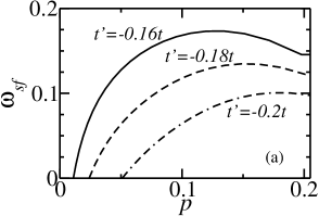
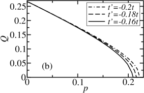
Figure 1: The spin-flip frequency $\omega_{sf}$ (a) and the RAF parameter $Q$ (b) are displayed versus doping for $U=2.8t$ and the values of three values of $t^{\prime}$ as shown. Temperature is $0.1t$. $n$ and $Q$ are calculated using RAFT’s mean-field equations (17).azzouz2003 ; azzouz2003p ; azzouz2004 The chemical potential $\mu$ is calculated versus doping $p=1-2n$ using the same equations.

We now discuss the results of the calculation of $\omega_{sf}$ as a function of doping for the Hamiltonian parameters $U=2.8t$ with three different values of $t^{\prime}$; $t^{\prime}=-0.16t$, $-0.18t$, and $-0.2t$. The temperature is $T=0.1t$. Fig. 1 displays the results of such calculations. The mean-field equations (17) were solved numerically using a C code. It is very interesting that $\omega_{sf}$ shows a doping dependence similar to that of the energy $E_{\rm cross}$ defined as the energy at the waist of the hour-glass spectrum displayed by the high-$T_{C}$ superconducting families La_2-xSr_xCuO₄, La_2-xBa_xCuO₄, YBa₂Cu₃O_6+x, and Bi₂Sr₂Cu₂O_8+δ (refer to Fig. 2 of Ref. fujita2012, for the hour-glass spectra and to Fig. 5 of the same reference for the doping dependence of $E_{\rm cross}$). In the underdoped regime, both $E_{\rm cross}$ and $\omega_{sf}$ increase with doping, reach a maximum at a doping below the optimal point, then decrease slightly. Note that $\omega_{sf}$ is meaningful only below the optimal doping because the RAF order disappears at a quantum critical point which coincides practically with this point.azzouz2003 This result is not in contradiction with some of the experimental results which also indicate that the resonance happens only in the uderdoped regime.fujita2012

IV Discussion

Together with the broken time-reversal symmetry observed in photoemission experiments,kaminski2002 polarized neutron diffraction experimentsfauque2006 ; li2008 indicated the universal existence of the ${\bf q}=0$ unusual magnetic order below $T^{*}$. In addition, the inelastic neutron scattering data reported for HgBa₂CuO_4+δ by Li et al.li2010 revealed a fundamental collective magnetic mode associated with this order. This collective mode seems to connect with the magnetic resonance that occurs at ${\bf Q}_{AF}=(\pi,\pi)$. If this connection is confirmed then the zero-momentum (${\bf q}=0$) order and the ${\bf Q}_{AF}$ resonance will have to be interpreted as two different signatures for the same physical phenomenon, which we propose here to be the rotating antiferromagnetic order. This suggests that the decoration of a unit cell with an even number of magnetic moments, like in Varma’s theory,varma1997 ; varma2006 would not be adequate, as this would rule out any staggered antiferromagnetic correlation at ${\bf Q}_{AF}$.

This claim is supported in our opinion by other experimental data collected so far within the PG, like the spin-like excitations reported in the single layer Bi_2+xSr_2-xCuO_6+δ,enoki2010 the static or quasi-static incommensurate spin order observed at low temperature in YBa₂Cu₃O_6+x with $x=0.45$ and $2\%$ Zn-doped $x=0.6$ crystals,hinkov2008 ; suchaneck2010 or the hour-glass spin excitationsfujita2012 reported in La_2-xSr_xCuO₄, La_2-xBa_xCuO₄, YBa₂Cu₃O_6+x, and Bi₂Sr₂Cu₂O_8+δ systems. All these results are interpreted in terms of excitations of the spin degrees of freedom.

Remnant magnetic excitations appear also to survive at higher energies in the underdoped phase. Above $E_{\rm cross}$ in the hour-glass spectrum, these excitations resemble the spin wave excitations in the undoped cuprate parents. Below $E_{\rm cross}$, the correlations lead however to new magnetic excitations. These results constitute also significant evidence for the nature and origin of these excitations being the spin degrees of freedom. All the above discussion and the results of the present work suggest that RAFT, which is based on spin antiferromagnetism, is a serious candidate for modeling the unusual magnetic properties. This adds to the fact that RAFT has been successfully used to model the electronic properties of the high-$T_{C}$ cuprates.

V conclusion

In summary, the neutron-scattering response expected from a state characterized by rotating antiferromagnetic order is calculated in this paper within the rotating antiferromagnetism theory. We argue that the resonance peak observed experimentally in the hole-doped high-$T_{C}$ cuprate superconductors is a consequence of the rotating antiferromagnetic order. We find that the phase of the order parameter of this order is responsible for the occurrence of a peak at a nonzero frequency, for which we estimated its doping dependence. The trends shown by this dependence are very similar to those of the doping dependence of the resonance energy or the energy $E_{\rm cross}$ at the waist of the magnetic excitations spectrum, namely the hour-glass spectra. The order parameter of the rotating antiferromagnetic order has a magnitude and a phase.azzouz2003 From this work and earlier ones,azzouz2013 it turns out that while the magnitude is responsible for the pseudogap behavior and other unusual thermodynamic and transport properties, the phase is responsible for the unusual magnetic properties of the high-$T_{C}$ cuprate materials, at least in the hole doped materials. If our present claim of RAFT being able to account for the unusual magnetic properties is confirmed by other independent works, then we will be one more step closer to the applicability of the rotating antiferromagnetism theory for the high-$T_{C}$ materials.

- (1) B. Fauqué, Y. Sidis, V. Hinkov, S. Pailhès, C.T. Lin, X. Chaud, and P. Bourges, Phys. Rev. Lett. 96, 197001 (2006).
- (2) Y. Li, V. Balédent, N. Barisic, Y. Cho, B. Fauqué, Y. Sidis, G. Yu, X. Zhao, P. Bourges, and M. Greven, Nature 455, 375 (2008).
- (3) T. Timusk, B. Statt, Rep. Prog. Phys. 62, 61 (1999).
- (4) For a review on the unusual magnetic properties of HTSCs refer to: Masaki Fujita, Haruhiro Hiraka, Masaaki Matsuda, Masato Matsuura, John M. Tranquada, Shuichi Wakimoto, Guangyong Xu, Kazuyoshi Yamada, J. Phys. Soc. Jpn. 81, 011007 (2012).
- (5) J. Rossat-Mignod, L.P. Regnault, C. Vettier, P. Bourges, P. Burlet, J. Bossy, J. Y. Henry, and G. Lapertot, Physica C 185-189, 86 (1991).
- (6) Y. Li, V. Bald́ent, G. Yu, N. Barisic, K. Hradil, R.A. Mole, Y. Sidis, P. Steffens, X. Zhao, P. Bourges, M. Greven, Nature 468, 283 (2010).
- (7) G. Yu, Y. Li, E. M. Motoyama, X. Zhao, N. Barisic, Y. Cho, P. Bourges, K. Hradil, R. A. Mole, and M. Greven, Phys. Rev. B 81, 064518 (2010).
- (8) M. P. M. Dean, R. S. Springell, C. Monney, K. J. Zhou, J. Pereiro, I. Bozovic, B. Dalla Piazza, H. M. Ronnow, E. Morenzoni, J. van den Brink, T. Schmitt, and J. P. Hill, Nature Materials 11, 850 (2012).
- (9) M. Azzouz, Phys. Rev. B 67, 134510 (2003).
- (10) M. Azzouz, Phys. Rev. B 68, 174523 (2003).
- (11) M. Azzouz, Phys. Rev. B 70, 052501 (2004).
- (12) H. Saadaoui, M. Azzouz, Phys. Rev. B 72, 184518 (2005).
- (13) M. Azzouz, K.C. Hewitt, H. Saadaoui, Phys. Rev. B 81, 174502 (2010).
- (14) M. Azzouz, B.W. Ramakko, G. Presenza-Pitman, J. Phys.: Condens. Matter 22, 345605 (2010).
- (15) E.H. Bhuiyan, G. Presenza-Pitman, M. Azzouz, Physica C 473, 61 (2012).
- (16) M. Azzouz, Physica C 480, 34 (2012).
- (17) M. Azzouz, Spectrum 5, 215 (2013).
- (18) Rui-Hua He, M. Hashimoto, H. Karapetyan, J.D. Koralek, J.P. Hinton, J.P. Testaud, V. Nathan, Y. Yoshida, Hong Yao, K. Tanaka, W. Meevasana, R.G. Moore, D. H. Lu, S.-K. Mo, M. Ishikado, H. Eisaki, Z. Hussain, T.P. Devereaux, S.A. Kivelson, J. Orenstein, A. Kapitulnik, Z.-X. Shen, Science 331, 1579 (2011).
- (19) C.M. Varma, Phys. Rev. B 55, 14554 (1997).
- (20) C.M. Varma, Phys. Rev. B 73, 155113 (2006).
- (21) S. Chakravarty, R.B. Laughlin, D.K. Morr, C. Nayak, Phys. Rev. B 63, 094503 (2001).
- (22) V.J. Emery and S.A. Kivelson, Nature 374, 434 (1995).
- (23) For all the quantities involved in this expression refer to: G.L. Squires, Introduction to the Thermal Neutron Scattering, Dover Publications, INC. 1978.
- (24) Private email communication (2013).
- (25) M. Enoki, M. Fujita, S. Iikubo, and K. Yamada, Physica C 470, S37 (2010).
- (26) A. Kaminski, S. Rosenkranz, H. M. Fretwell, J. C. Campuzano, Z. Li, H. Raffy, W. G. Cullen, H. You, C. G. Olson, C. M. Varma, and H. Hochst, Nature 416, 610 (2002).
- (27) V. Hinkov, D. Haug, B. Fauqué, P. Bourges, Y. Sidis, A. Ivanov, C. Bernhard, C. T. Lin, and B. Keimer, Science 319, 597 (2008).
- (28) A. Suchaneck, V. Hinkov, D. Haug, L. Schulz, C. Bernhard, A. Ivanov, K. Hradil, C. T. Lin, P. Bourges, B. Keimer, and Y. Sidis, Phys. Rev. Lett. 105, 037207 (2010).