Impact of delay on HIV-1 dynamics of fighting a virus with another virus

Abstract.

In this paper, we propose a mathematical model for HIV-1 infection with intracellular delay. The model examines a viral-therapy for controlling infections through recombining HIV-1 virus with a genetically modified virus. For this model, the basic reproduction number $\mathcal{R}_{0}$ are identified and its threshold properties are discussed. When $\mathcal{R}_{0}<1$, the infection-free equilibrium $E_{0}$ is globally asymptotically stable. When $\mathcal{R}_{0}>1$, $E_{0}$ becomes unstable and there occurs the single-infection equilibrium $E_{s}$, and $E_{0}$ and $E_{s}$ exchange their stability at the transcritical point $\mathcal{R}_{0}=1$. If $1<\mathcal{R}_{0}<R_{1}$, where $R_{1}$ is a positive constant explicitly depending on the model parameters, $E_{s}$ is globally asymptotically stable, while when $\mathcal{R}_{0}>R_{1}$, $E_{s}$ loses its stability to the double-infection equilibrium $E_{d}$. There exist a constant $R_{2}$ such that $E_{d}$ is asymptotically stable if $R_{1}<\mathcal{R}_{0}<R_{2}$, and $E_{s}$ and $E_{d}$ exchange their stability at the transcritical point $\mathcal{R}_{0}=R_{1}$. We use one numerical example to determine the largest range of $\mathcal{R}_{0}$ for the local stability of $E_{d}$ and existence of Hopf bifurcation. Some simulations are performed to support the theoretical results. These results show that the delay plays an important role in determining the dynamic behaviour of the system. In the normal range of values, the delay may change the dynamic behaviour quantitatively, such as greatly reducing the amplitudes of oscillations, or even qualitatively changes the dynamical behaviour such as revoking oscillating solutions to equilibrium solutions. This suggests that the delay is a very important fact which should not be missed in HIV-1 modelling.

Yun Tian, Yu Bai, Pei Yu

Department of Applied Mathematics,

Western University, London, Ontario N6A 5B7, Canada

(Communicated by the associate editor name)

1. Introduction

Human immunodeficiency virus (HIV) is a serious mortal lentivirus, which can cause acquired immunodeficiency syndrome (AIDS). Reports have known that many people are killed by AIDS every year, and yet, until today, there is no effective way to cure the AIDS. Thus, many scientists and researchers have been focusing on the study of controlling the infections. One of the approaches developed recently, offered by genetic engineering, is to use recombinant virus capable of controlling infections of HIV [15, 12]. Recently, Revilla and Garcia-Ramos established a 5-dimensional ordinary differential system to investigate the control of the infections by introducing a recombinant virus to fight the virus [13]. Later, this model was studied by Jiang et al. [6] in detail to show various bifurcation patters and rich dynamics, as well as a control study given in [18] by introducing a constant injection rate of the recombinant virus to this model.

A standard and classic in-host model for HIV infection can be described by the following differential equations:

$$\begin{array}[]{lll}\dot{x}&\!\!\!=\!\!\!&\lambda-dx-\beta xv,\\[0.0pt] \dot{y}&\!\!\!=\!\!\!&\beta xv-ay,\\[0.0pt] \dot{v}&\!\!\!=\!\!\!&ky-pv,\end{array}$$ (1)

where $x(t)$, $y(t)$, $v(t)$ are the density of virus-free host cells, infected cells, and a pathogen virus, respectively, at time $t$. The production rate and death rate for the healthy cells are respectively $\lambda$ and $d$. $\beta$ is the constant rate at which a T-cell is contacted by the virus. It is also assumed that once cells are infected, they may die at a rate $a$ due to the action of either the virus or the immune system, and each produces the pathogens at a rate $k$ during their life which on average has length $1/a$.

In [13], a second virus is added into model (1) which may cause the infected cells to have a second infection, called double-infection, leading to a modified model as

$$\begin{array}[]{cll}\dot{x}&\!\!\!=\!\!\!&\lambda-dx-\beta xv,\\[0.0pt] \dot{y}&\!\!\!=\!\!\!&\beta xv-ay-\alpha wy,\\[0.0pt] \dot{z}&\!\!\!=\!\!\!&\alpha wy-bz,\\[0.0pt] \dot{v}&\!\!\!=\!\!\!&ky-pv,\\[0.0pt] \dot{w}&\!\!\!=\!\!\!&cz-qw,\end{array}$$ (2)

where $w(t)$ and $z(t)$ are the recombinant (genetically modified) virus and double-infected cells. After the second virus is enrolled, once the cells which have been infected by the pathogens are infected again by the recombinant, they can be turned into double-infected cells at a rate $\alpha\omega y$, where the recombinants are removed at a rate $qw$. The double infected cells die at a rate $bz$, and release recombinants at rate $cz$. Having established the model (2), the authors of [13] analyzed the structure of equilibrium solutions and presented some simulations. Later, in [6], the authors fully analyzed the stability of all three equilibrium solutions and bifurcations between these equilibria, as well as proved the existence of Hopf bifurcation. Further, in [18], the fifth equation of model (2) is modified as $\dot{w}=\eta+cz-qw$, where $\eta$ is a control parameter to measure the injection rate of the recombinant, and then a complete dynamical analysis is given in this article, showing that increasing $\eta$ is beneficial for controlling/eliminating the HIV virus [18].

In this paper, to further improve the model (2), we introduce a time lag into the model (2), since in real situation, time is needed for the virus to contact a target cell and then the contacted cells to become actively affected. This can be described by the eclipse phase of the virus life cycle. Moreover, we assume that the probability density that a cell still remains infected for $\tau$ time units after being contacted by the virus obeys an exponentially decay function. Therefore, following the line of [17, 19], model (2) can be modified to

$$\begin{array}[]{cll}\dot{x}(t)&\!\!\!=\!\!\!&\lambda-dx(t)-\beta x(t)v(t),\\[1.42262pt] \dot{y}(t)&\!\!\!=\!\!\!&\beta e^{-a\tau}x(t-\tau)v(t-\tau)-ay(t)-\alpha w(t)y(t),\\[1.42262pt] \dot{z}(t)&\!\!\!=\!\!\!&\alpha w(t)y(t)-bz(t),\\[1.42262pt] \dot{v}(t)&\!\!\!=\!\!\!&ky(t)-pv(t),\\[1.42262pt] \dot{w}(t)&\!\!\!=\!\!\!&cz(t)-qw(t),\end{array}$$ (3)

where $\tau$ denotes the average time for a viral particle to go through the eclipse phase. Because the dimension of the system is higher than two, model (3) may exhibit some interesting dynamic behaviors (Hopf bifurcation, limit cycles and even chaos), which would make the analysis of the system more complicated. Thus, the main goal of this paper focuses on dynamical behaviour of the system with delay, in particular, on equilibrium solutions and their bifurcations. More importantly, we want to find the impact of the delay on the dynamical properties.

The rest of this paper is organized as follows. In next section, for system (3) we will discuss the well-posedness of the solutions, equilibria and their stability. Also, in order to properly define biologically meaningful equilibria, the basic reproduction number $\mathcal{R}_{0}$ will be defined. In Sections 3, 4 and 5, we analyze the stability of the three equilibria: disease-free equilibrium $E_{0}$ , single-infection equilibrium $E_{s}$, and double-infection equilibrium $E_{d}$. It will be shown that $E_{0}$ is globally asymptotically stable for $0<\mathcal{R}_{0}<1$, $E_{s}$ is globally asymptotically stable for $1<\mathcal{R}_{0}<R_{1}$, where $R_{1}>1$ is a constant defined in terms of the system parameters, and $E_{d}$ is asymptotically stable for $R_{1}<\mathcal{R}_{0}<R_{h}$, where $R_{h}$ denotes a Hopf critical point from which a family of limit cycles bifurcate. A numerical example is present in Section 6 to demonstrate the theoretical predictions. Finally, conclusion and discussion are drawn in Section 7.

2. Well-posedness, boundedness of solutions, equilibria and basic reproduction number

Because of biological reasons, all variables in model (3) must be non-negative. Therefore, for any non-negative initial values, the corresponding solution must remain non-negative. We have the following result.

Theorem 2.1.

All solutions of system (3) remain non-negative, provided the given conditions are non-negative, and bounded.

Proof.

For convenience, let $X=C([-\tau,0];R^{5})$ be the Banach space of continuous mapping from $[-\tau,0]$ to $R^{5}$ equipped with the sup-norm. Let $\mathbf{x}(t)=(x(t),y(t),z(t),\\ v(t),w(t))^{T}$ and $\mathbf{x}_{t}(\theta)=\mathbf{x}(t+\theta)$ for $\theta\in[-\tau,0]$. By the fundamental theory of FDEs (see, e.g. [4]), for any initial condition $\phi\in X$ with $\phi\geq 0$, we know that there exists a unique solution $\mathbf{x}(t,\phi)$ satisfying $\mathbf{x}(\theta,\phi)=\phi(\theta)$, $\theta\in[-\tau,0]$.

System (3) can be written as $\dot{\mathbf{x}}(t)=\mathbf{f}(\mathbf{x}_{t})$, where

$$\mathbf{f}(\mathbf{x}_{t})=\left(\begin{array}[]{c}\lambda-dx_{t}(0)-\beta x_{t}(0)v_{t}(0)\\ \beta e^{-a\tau}x_{t}(-\tau)v_{t}(-\tau)-ay_{t}(0)-\alpha w_{t}(0)y_{t}(0)\\ \alpha w_{t}(0)y_{t}(0)-bz_{t}(0)\\ ky_{t}(0)-pv_{t}(0)\\ cz_{t}(0)-qw_{t}(0)\end{array}\right).$$

It is easy to see that if any $\phi\in X$ satisfies $\phi\geq 0$, $\phi_{i}(0)=0$ for some $i$, then $\mathbf{f}_{i}(\phi)\geq 0$. Therefore, according to Theorem 2.1 (on page 81) in [14] we know that $\mathbf{x}(t,\phi)\geq 0$ for all $t\geq 0$ in its maximal interval of existence if $\phi\geq 0$.

Next, to show the boundedness of the solution $(x(t),y(t),z(t),v(t),w(t))$, we define

$$B(t)=cke^{-a\tau}x(t)+cky(t+\tau)+ckz(t+\tau)+\frac{ac}{2}v(t+\tau)+\frac{bk}{2}w(t+\tau).$$

Then, the derivative of $B(t)$ with respective to time $t$ along the solution of trajectory of system (3) is given by

$$\begin{split}\frac{dB(t)}{dt}\Big{|}_{(\ref{b3})}=&\ cke^{-a\tau}\big{[}\lambda-dx(t)-\beta v(t)x(t)\big{]}\\[-4.30554pt] &+ck\big{[}\beta e^{-a\tau}v(t)x(t)-ay(t+\tau)-\alpha w(t+\tau)y(t+\tau)\big{]}\\ &+ck\big{[}\alpha w(t+\tau)y(t+\tau)-bz(t+\tau)\big{]}\\[-2.15277pt] &+\frac{ac}{2}\big{[}ky(t+\tau)-pv(t+\tau)\big{]}+\frac{bk}{2}\big{[}cz(t+\tau)-qw(t+\tau)\big{]}\\[-4.30554pt] =&\ cke^{-a\tau}\lambda-dcke^{-a\tau}x(t)-\frac{a}{2}cky(t+\tau)-\frac{b}{2}ckz(t+\tau)\\[-4.30554pt] &-p\frac{ac}{2}v(t+\tau)-q\frac{bk}{2}w(t+\tau)\\ \leq&\ cke^{-a\tau}\lambda-mB(t)\left\{\!\!\begin{array}[]{ll}<0&{\rm for}\ \ B(t)>\displaystyle\frac{ck}{m}e^{-a\tau},\\[6.45831pt] >0&{\rm for}\ \ B(t)<\displaystyle\frac{ck}{m}e^{-a\tau},\end{array}\right.\end{split}$$

where $m=\min\{d,\frac{a}{2},\frac{b}{2},p,q\}$ This implies that $B(t)$ is bounded, so are $x(t)$, $y(t)$, $z(t)$, $v(t)$ and $w(t)$. ∎

Model (3) has three possible biologically meaningful equilibria: disease-free equilibrium $E_{0}$, single-infection equilibrium $E_{s}$ and double-infection equilibrium $E_{d}$, given below:

$$\begin{split}E_{0}=&\Big{(}\frac{\lambda}{d},\,0,\,0,\,0,\,0\Big{)},\\ E_{s}=&\Big{(}\frac{ap}{\beta ke^{-a\tau}},\ \frac{k\beta\lambda e^{-a\tau}-adp}{\beta ak},\ 0,\ \frac{k\beta\lambda e^{-a\tau}-adp}{\beta ap},\ 0\Big{)},\\ E_{d}=&\Big{(}\frac{\lambda\alpha cp}{d\alpha cp+\beta bkq},\ \frac{bq}{\alpha c},\ \frac{q(\alpha\beta\lambda cke^{-a\tau}-\beta abkq-\alpha acdp)}{\alpha c(\beta bkq+\alpha cdp)},\\ &\quad\frac{bkq}{\alpha cp},\ \frac{\alpha\beta\lambda cke^{-a\tau}-\beta abkq-\alpha acdp}{\alpha(\beta bkq+\alpha cdp)}\Big{)}.\end{split}$$

We define

$$\mathcal{R}_{0}\triangleq\frac{\lambda}{d}\cdot\frac{\beta e^{-a\tau}}{a}\cdot\frac{k}{p}=\frac{k\beta\lambda}{adp}e^{-a\tau},$$

where $\frac{\lambda}{d}$ is the average number of healthy cells available for infection, $\frac{\beta e^{-a\tau}}{a}$ is the average number of host cells that each HIV virus infects, and $\frac{k}{p}$ is the average number of HIV viruses that an infected cell produces. Therefore, $\mathcal{R}_{0}$ is the basic reproduction number.

It is seen that the disease-free equilibrium is independent of the delay. If $\mathcal{R}_{0}<1$, $E_{0}$ is the only biologically meaningful equilibrium. If $\mathcal{R}_{0}>1$, there is another biologically meaningful equilibrium $E_{s}$ (single-infection equilibrium). The double-infection equilibrium $E_{d}$ exists (biologically meaningful) if and only if $R_{d}>1$, where

$$R_{d}=\frac{\alpha\beta\lambda cke^{-a\tau}-\alpha acdp}{\beta abkq}=\frac{\alpha cdp}{\beta bkq}(\mathcal{R}_{0}-1).$$

Hence,

$$R_{d}>1\Leftrightarrow\mathcal{R}_{0}>R_{1},\ \ \mbox{where}\ R_{1}=1+\frac{\beta bkq}{\alpha cdp}.$$

Note that $R_{1}$ is independent of the delay.

3. Stability of the disease-free equilibrium $E_{0}$

First, for the local stability of $E_{0}$, we have the following theorem.

Theorem 3.1.

When $\mathcal{R}_{0}<1$, the disease-free equilibrium $E_{0}$ is locally asymptotically stable; when $\mathcal{R}_{0}>1$, $E_{0}$ becomes unstable and the single-infection equilibrium $E_{s}$ occurs.

Proof.

The linearized system of (3) at the disease-free equilibrium $E_{0}$ is

$$\begin{array}[]{cll}\dot{x}(t)&\!\!\!=\!\!\!&-dx(t)-\frac{\beta\lambda}{d}v(t),\\[2.84526pt] \dot{y}(t)&\!\!\!=\!\!\!&\beta e^{-a\tau}\frac{\lambda}{d}v(t-\tau)-ay(t),\\[2.84526pt] \dot{z}(t)&\!\!\!=\!\!\!&-bz(t),\\[1.42262pt] \dot{v}(t)&\!\!\!=\!\!\!&ky(t)-pv(t),\\[0.0pt] \dot{w}(t)&\!\!\!=\!\!\!&cz(t)-qw(t),\end{array}$$

for which the characteristic equation is given by

$$(\xi+d)(\xi+b)(\xi+q)\Big{[}\xi^{2}+(a+p)\xi+ap-\frac{\beta\lambda k}{d}e^{-(a+\xi)\tau}\Big{]}=0.$$

Obviously, for the local stability of $E_{0}$, it suffices to only consider the following equation

$$D_{0}(\xi)=\xi^{2}+(a+p)\xi+ap-\frac{\beta\lambda k}{d}e^{-(a+\xi)\tau}=0.$$ (4)

If $\mathcal{R}_{0}>1$, it is easy to show for real $\xi$ that

$$D_{0}(0)=ap(1-\mathcal{R}_{0})<0,\quad\lim_{\xi\rightarrow+\infty}D_{0}({\xi})=+\infty.$$

Hence, $D_{0}(\xi)=0$ has at least one positive real root. Therefore, if $\mathcal{R}_{0}>1$, the infection-free equilibrium $E_{0}$ is unstable.

Next, consider $\mathcal{R}_{0}<1$. When $\tau=0$, equation (4) becomes

$$\xi^{2}+(a+p)\xi+ap-\frac{\beta\lambda k}{d}=0.$$ (5)

In order for the two roots of (5) to have negative real part, it requires $ap-\beta\lambda k/d>0$, which is equivalent to $\mathcal{R}_{0}|_{\tau=0}<1$. Thus, all the roots of (5) have negative real part when $\mathcal{R}_{0}<1$. From [2], we know that all the roots of (4) continuously depend on $\tau$. And the assumption

$$\limsup\left\{\left|\frac{Q(\xi,\tau)}{P(\xi,\tau)}\right|:|\xi|\rightarrow\infty,\ {\rm Re}(\xi)\geq 0\right\}<1,\ \ {\rm for}\ {\rm any}\ \tau,$$ (6)

could ensure that there are no roots existing in the infinity for equations in the form $P(\xi,\tau)+Q(\xi,\tau)e^{-\xi\tau}=0$ (see [1]). Obviously, (6) holds here for (4), and hence ${\rm Re}(\xi)<+\infty$ for any root $\xi$ of (4) when $\mathcal{R}_{0}<1$. As a result, for $\mathcal{R}_{0}<1$, the only possibility for the roots of equation (4) to enter into the right half plane is to cross the imaginary axis when $\tau$ increases. Thus, we define $\xi=i\varpi$, $(\varpi>0)$, to be a purely imaginary root of (4). Then we get

$$-\varpi^{2}+i(a+p)\varpi+ap-\frac{k\beta\lambda}{d}e^{-(a+i\varpi)\tau}=0.$$ (7)

Taking moduli of (7) gives

$$H_{0}(\varpi^{2})=\varpi^{4}+(a^{2}+p^{2})\varpi^{2}+a^{2}p^{2}-\Big{(}\frac{k\beta\lambda}{d}e^{-a\tau}\Big{)}^{2}=0.$$

Clearly, $H_{0}(\varpi^{2})$ has no positive real roots if $\mathcal{R}_{0}<1$. Therefore, all the roots of (4) have negative real part if $\mathcal{R}_{0}<1$. ∎

Further, for the global stability of $E_{0}$, we have the following result.

Theorem 3.2.

If $\mathcal{R}_{0}<1$, the disease-free equilibrium $E_{0}$ is globally asymptotically stable, implying that none of the two virus can invade regardless of the initial load.

Proof.

We construct the following Lyapunov function:

$$\begin{split}V_{0}=&\ \frac{e^{-a\tau}}{2}\Big{[}x(t)-\frac{\lambda}{d}\Big{]}^{2}+\frac{\lambda}{d}y(t)+\frac{\lambda}{d}z(t)+\frac{a\lambda}{dk}v(t)+\frac{b\lambda}{cd}w(t)\\ &+\frac{\lambda\beta}{d}e^{-a\tau}\int_{t-\tau}^{t}{x(\eta)v(\eta)}d\eta.\end{split}$$

Using non-negativity of the solution and $\mathcal{R}_{0}<1$, the derivative of $V_{0}$ with respective to time $t$ along the solution of system (3) can be expressed as

$$\begin{split}\frac{dV_{0}}{dt}\Big{|}_{(\ref{b3})}=&\ e^{-a\tau}\Big{[}x(t)-\frac{\lambda}{d}\Big{]}\big{[}\lambda-dx(t)-\beta v(t)x(t)\big{]}\\ &+\frac{\lambda}{d}\big{[}\beta e^{-a\tau}x(t-\tau)v(t-\tau)-ay(t)-bz(t)\big{]}\\ &+\frac{a\lambda}{dk}\big{[}ky(t)-pv(t)\big{]}+\frac{b\lambda}{cd}\big{[}cz(t)-qw(t)\big{]}\\ &+\frac{\lambda\beta}{d}e^{-a\tau}\big{[}x(t)v(t)-x(t-\tau)v(t-\tau)\big{]}\\ =&-e^{-a\tau}\Big{[}x(t)-\frac{\lambda}{d}\Big{]}^{2}\big{[}d+\beta v(t)\big{]}-\Big{[}\frac{a\lambda}{dk}p-\frac{\lambda^{2}}{d^{2}}\beta e^{-a\tau}\Big{]}v(t)-\frac{bq\lambda}{cd}w(t)\\ =&-e^{-a\tau}\Big{[}x(t)-\frac{\lambda}{d}\Big{]}^{2}\big{[}d+\beta v(t)\big{]}-\frac{ap\lambda}{dk}(1-\mathcal{R}_{0})v(t)-\frac{bq\lambda}{cd}w(t)\\ \leq&\ 0,\end{split}$$

and the equality holds for $x=\frac{\lambda}{d}$, $v=w=0$. Thus, by LaSalle’s invariance principle [8], we conclude that $E_{0}$ is globally asymptotically stable. ∎

4. Stability of the single-infection equilibrium $E_{s}$

From the analysis given in the previous section, we know that at the critical point $\mathcal{R}_{0}=1$, the disease-free equilibrium $E_{0}$ becomes unstable and bifurcates into the single-infection equilibrium $E_{s}$, which exists for $\mathcal{R}_{0}>1$. Thus, in order to study the stability of $E_{s}$, we assume $\mathcal{R}_{0}>1$ in this section. Similarly, for the local stability of $E_{s}$, we have the following result.

Theorem 4.1.

If $1<\mathcal{R}_{0}<R_{1}$, the single-infection equilibrium $E_{s}$ is asymptotically stable; when $\mathcal{R}_{0}>R_{1}$, $E_{s}$ becomes unstable.

Proof.

The linearized system of model (3) at $E_{s}=(x_{s},y_{s},0,v_{s},0)$ is

$$\begin{array}[]{cll}\dot{x}(t)&\!\!\!=\!\!\!&-(d+\beta v_{s})x(t)-\beta x_{s}v(t),\\[2.84526pt] \dot{y}(t)&\!\!\!=\!\!\!&\beta e^{-a\tau}\big{[}v_{s}x(t-\tau)+x_{s}v(t-\tau)\big{]}-ay(t)-\alpha y_{s}w(t),\\[2.84526pt] \dot{z}(t)&\!\!\!=\!\!\!&\alpha y_{s}w(t)-bz(t),\\[1.42262pt] \dot{v}(t)&\!\!\!=\!\!\!&ky(t)-pv(t),\\[1.42262pt] \dot{w}(t)&\!\!\!=\!\!\!&cz(t)-qw(t),\end{array}$$

with the corresponding characteristic equation given by $D_{1}(\xi)D_{2}(\xi)=0$, where

$$\begin{split}D_{1}(\xi)=&\ \xi^{2}+(b+q)\xi+bq-\frac{c\alpha(k\beta\lambda e^{-a\tau}-adp)}{\beta ak},\\ D_{2}(\xi)=&\ \xi^{3}+\Big{(}a+p+\frac{k\beta\lambda}{ap}e^{-a\tau}\Big{)}\xi^{2}+\Big{[}\frac{k\beta\lambda}{ap}e^{-a\tau}(a+p)+ap\Big{]}\xi\\ &\quad+k\beta\lambda e^{-a\tau}-ap(\xi+d)e^{-\xi\tau}.\end{split}$$

First, note that $D_{1}(\xi)$ can be rewritten as

$$D_{1}(\xi)=\xi^{2}+(b+q)\xi+bq(1-R_{d}),$$

which indicates that $D_{1}(\xi)=0$ has two roots with negative real part if and only if $R_{d}<1$ (i.e. $\mathcal{R}_{0}<R_{1}$), or one positive root and one negative if $R_{d}>1$ (i.e. $\mathcal{R}_{0}>R_{1}$). Therefore, if $\mathcal{R}_{0}>R_{1}$, the single-infection equilibrium $E_{s}$ is unstable.

For $D_{2}(\xi)=0$, we rewrite it as

$$\begin{array}[]{lll}\xi^{3}+a_{2}(\tau)\xi^{2}+a_{1}(\tau)\xi+a_{0}(\tau)-(c_{1}\xi+c_{2})e^{-\xi\tau}=0,\end{array}$$ (8)

where

$$\begin{split}a_{2}(\tau)&=a+p+\frac{k\beta\lambda}{ap}e^{-a\tau},\quad a_{1}(\tau)=\frac{k\beta\lambda}{ap}e^{-a\tau}(a+p)+ap,\\ a_{0}(\tau)&=k\beta\lambda e^{-a\tau},\quad c_{1}=ap,\quad c_{2}=apd.\end{split}$$

It is easy to see that $\xi=0$ is not a root of (8) if $\mathcal{R}_{0}>1$, since

$$a_{0}(\tau)-c_{2}=k\beta\lambda e^{-a\tau}-apd=apd(\mathcal{R}_{0}-1)>0.$$

When $\tau=0$, (8) becomes

$$\xi^{3}+a_{2}(0)\xi^{2}+(a_{1}(0)-c_{1})\xi+a_{0}(0)-c_{2}=0.$$ (9)

Applying the Routh-Hurwitz criterion (see [3]), we know that all the roots of (9) have negative real part, because

$$\begin{split}&a_{2}(0)=a+p+\frac{k\beta\lambda}{ap}>0,\\ &a_{1}(0)-c_{1}=\frac{k\beta\lambda}{ap}(a+p)>0,\\ &a_{0}(0)-c_{2}=k\beta\lambda-apd=apd(\mathcal{R}_{0}|_{\tau=0}-1)>0,\end{split}$$

and

$$\begin{split}a_{2}(0)(a_{1}(0)\!-\!c_{1})-(a_{0}(0)\!-\!c_{2})=&\ \Big{(}a+p+\frac{k\beta\lambda}{ap}\Big{)}\frac{k\beta\lambda}{ap}(a+p)-(k\beta\lambda-apd)\\ =&\ \frac{k^{2}\beta^{2}\lambda^{2}}{a^{2}p^{2}}(a+p)+\frac{k\beta\lambda}{ap}(a^{2}+ap+p^{2})+apd>0.\end{split}$$

Therefore, any root of (8) has negative real part when $\tau=0$. As discussed in Section 3, we know that all the roots of equation (8) depend continuously on $\tau$. Also, (6) holds for (8), and hence ${\rm Re}(\xi)<+\infty$ if $D_{2}(\xi)=0$. Then, the roots of equation (8) can only enter into the right half plane by crossing the imaginary axis when $\tau$ increases. Thus, we define $\xi=i\varpi$ ($\varpi>0$) to be a purely imaginary root of (8), and then obtain

$$-i\varpi^{3}-a_{2}(\tau)\varpi^{2}+ia_{1}(\tau)\varpi+a_{0}(\tau)-(ic_{1}\varpi+c_{2})e^{-i\varpi\tau}=0,$$

Taking moduli of the above equation results in

$$\begin{split}H_{s}(\varpi^{2})=\varpi^{6}&+\big{[}a_{2}^{2}(\tau)-2a_{1}(\tau)\big{]}\varpi^{4}\\ &+\big{[}a_{1}^{2}(\tau)-2a_{0}(\tau)a_{2}(\tau)-c_{1}^{2}\big{]}\varpi^{2}+a_{0}^{2}(\tau)-c_{2}^{2}=0.\end{split}$$ (10)

Since

$$\begin{array}[]{lll}a_{2}^{2}(\tau)-2a_{1}(\tau)=a^{2}+p^{2}+d^{2}\mathcal{R}_{0}^{2}>0,\\[4.2679pt] a_{1}^{2}(\tau)-2a_{0}(\tau)a_{2}(\tau)-c_{1}^{2}=d^{2}(a^{2}+p^{2})\mathcal{R}_{0}^{2}>0,\\[4.2679pt] a_{0}(\tau)^{2}-c_{2}^{2}=a^{2}p^{2}d^{2}(\mathcal{R}_{0}^{2}-1)>0,\end{array}$$

all the coefficients of $H_{s}(\varpi^{2})$ are positive. Then the function $H_{s}(\varpi^{2})$ is monotonically increasing for $0\leq\varpi^{2}<\infty$ with $H_{s}(0)>0$. This implies that equation (10) has no positive roots if $\mathcal{R}_{0}>1$. Hence, all the roots of (8) have negative real part for $\tau>0$ if $\mathcal{R}_{0}>1$. ∎

Also, we we can show the global stability of $E_{s}$, as given in the following theorem.

Theorem 4.2.

If $1<\mathcal{R}_{0}<R_{1}$, the single-infection equilibrium $E_{s}$ is globally asymptotically stable, implying that the recombinant virus can not survive but the pathogen virus can.

Proof.

We construct the Lyapunov function $V_{s}=V_{1}+\beta x_{s}v_{s}e^{-a\tau}V_{2}$ with

$$\begin{split}V_{1}&=e^{-a\tau}(x-x_{s}\ln{x})+(y-y_{s}\ln{y})+z+\frac{a}{k}(v-v_{s}\ln v)+\frac{b}{c}w,\\ V_{2}&=\int_{t-\tau}^{t}\Big{(}\frac{x(\eta)v(\eta)}{x_{s}v_{s}}-\ln\frac{x(\eta)v(\eta)}{x_{s}v_{s}}\Big{)}d\eta.\end{split}$$

Substituting $E_{s}$ into (3) yields three identities $G_{i}\equiv 0$, $i=1,2,3$, where $G_{1}=\lambda-dx_{s}-\beta x_{s}v_{s}$, $G_{2}=\beta e^{-a\tau}x_{s}v_{s}-ay_{s}$, $G_{3}=ky_{s}-pv_{s}$. Then we have

$$\begin{split}V_{1,x}\dot{x}&=V_{1,x}\dot{x}-e^{-a\tau}\Big{(}1-\frac{x_{s}}{x}\Big{)}G_{1}-\frac{v}{v_{s}}G_{2}-\frac{av}{kv_{s}}G_{3}\\ &=dx_{s}e^{-a\tau}\Big{(}2-\frac{x_{s}}{x}-\frac{x}{x_{s}}\Big{)}+\beta x_{s}v_{s}e^{-a\tau}\Big{(}1-\frac{x_{s}}{x}-\frac{xv}{x_{s}v_{s}}\Big{)}+\frac{ap}{k}v,\\ V_{1,y}\dot{y}&=V_{1,y}\dot{y}+G_{2}\\ &=\beta x_{s}v_{s}e^{-a\tau}\Big{[}1+\frac{(y-y_{s})x(t-\tau)v(t-\tau)}{yx_{s}v_{s}}\Big{]}-ay+\alpha(y_{s}-y)w,\\ V_{1,v}\dot{v}&=V_{1,v}\dot{v}+\Big{(}1-\frac{yv_{s}}{y_{s}v}\Big{)}G_{2}+\frac{a}{k}G_{3}=\beta x_{s}v_{s}e^{-a\tau}\Big{(}1-\frac{yv_{s}}{y_{s}v}\Big{)}+ay-\frac{ap}{k}v,\\ V_{1,z}\dot{z}&=\alpha yw-bz,\qquad V_{1,w}\dot{w}=bz-\frac{bq}{c}w,\end{split}$$

which yields

$$\begin{split}&\ V_{1,x}\dot{x}+V_{1,y}\dot{y}+V_{1,z}\dot{z}+V_{1,v}\dot{v}+V_{1,w}\dot{w}\\ =&\ \beta x_{s}v_{s}e^{-a\tau}\Big{[}3-\frac{x_{s}}{x}-\frac{yv_{s}}{y_{s}v}+\frac{(y-y_{s})x(t-\tau)v(t-\tau)}{yx_{s}v_{s}}-\frac{xv}{x_{s}v_{s}}\Big{]}\\ &+dx_{s}e^{-a\tau}\Big{(}2-\frac{x_{s}}{x}-\frac{x}{x_{s}}\Big{)}+\frac{\alpha dp}{\beta k}(\mathcal{R}_{0}-R_{1})w,\end{split}$$ (11)

where $y_{s}=\frac{dp}{\beta k}(\mathcal{R}_{0}-1)$ has been used. And for $V_{2}$, we have

$$\frac{dV_{2}}{dt}=\frac{xv}{x_{s}v_{s}}-\frac{x(t-\tau)v(t-\tau)}{x_{s}v_{s}}+\ln\frac{x(t-\tau)v(t-\tau)}{xv}.$$ (12)

Combining (11) and (12) yields

$$\begin{split}\frac{dV_{s}}{dt}\Big{|}_{(3)}&=V_{1,x}\dot{x}+V_{1,y}\dot{y}+V_{1,z}\dot{z}+V_{1,v}\dot{v}+V_{1,w}\dot{w}+\beta x_{s}v_{s}e^{-a\tau}\frac{dV_{2}}{dt}\\ &=dx_{s}e^{-a\tau}\Big{(}2-\frac{x_{s}}{x}-\frac{x}{x_{s}}\Big{)}+\frac{\alpha dp}{\beta k}(\mathcal{R}_{0}-R_{1})w+\beta x_{s}v_{s}e^{-a\tau}W,\end{split}$$

where

$$W=3-\frac{x_{s}}{x}-\frac{yv_{s}}{y_{s}v}-\frac{y_{s}x(t-\tau)v(t-\tau)}{yx_{s}v_{s}}+\ln\frac{x(t-\tau)v(t-\tau)}{xv}\leq 0,$$

because the following inequality

$$n-\sum_{i=1}^{n}\frac{b_{i}}{a_{i}}+\ln\prod_{i=1}^{n}\frac{b_{i}}{a_{i}}\leq 0,$$

holds for any positive $a_{i}$ and $b_{i}$ (see [7]). Therefore, $\frac{dV_{s}}{dt}|_{(3)}\leq 0$ when $\mathcal{R}_{0}<R_{1}$, and the equality holds when $x=x_{s}$, $y=y_{s}$, $v=v_{s}$, $w=0$. Then, by LaSalle’s invariance principle [8], we conclude that $E_{s}$ is globally asymptotically stable. ∎

5. Stability of the double-infection equilibrium $E_{d}$

At the critical point $\mathcal{R}_{0}=R_{1}$, the single-infection equilibrium $E_{s}$ becomes unstable and the double-infection equilibrium $E_{d}$ comes into existence for $\mathcal{R}_{0}>R_{1}$. To discuss the stability of $E_{d}$, we assume $\mathcal{R}_{0}>R_{1}$ in this section. We have the following result for the stability of $E_{d}$.

Theorem 5.1.

For model $(\ref{b3})$, there exists an $R_{2}>R_{1}$ such that the double-infection equilibrium $E_{d}$ is asymptotically stable for $R_{1}<\mathcal{R}_{0}<R_{2}$.

Proof.

The linearized system of (3) at $E_{d}=(x_{d},y_{d},z_{d},v_{d},w_{d})$ is

$$\begin{array}[]{cll}\dot{x}(t)&\!\!\!=\!\!\!&-(d+\beta v_{d})x(t)-\beta x_{d}v(t),\\[2.84526pt] \dot{y}(t)&\!\!\!=\!\!\!&\beta e^{-a\tau}\big{[}v_{d}x(t-\tau)+x_{d}v(t-\tau)\big{]}-(a+\alpha w_{d})y(t)-\alpha y_{d}w(t),\\[2.84526pt] \dot{z}(t)&\!\!\!=\!\!\!&\alpha w_{d}y(t)-bz(t)+\alpha y_{d}w(t),\\[2.84526pt] \dot{v}(t)&\!\!\!=\!\!\!&ky(t)-pv(t),\\[2.84526pt] \dot{w}(t)&\!\!\!=\!\!\!&cz(t)-qw(t).\end{array}$$ (13)

By straightforward but tedious algebraic manipulations, we obtain the characteristic equation of (13), given by

$$\begin{split}D(\xi)=&\ (\xi+p)(\xi+dR_{1})\Big{[}\xi(\xi+b+q)\Big{(}\xi+a\frac{\mathcal{R}_{0}}{R_{1}}\Big{)}+abq\Big{(}\frac{\mathcal{R}_{0}}{R_{1}}-1\Big{)}\Big{]}\\ &-ap\frac{\mathcal{R}_{0}}{R_{1}}\xi(\xi+d)(\xi+b+q)e^{-\xi\tau}\\ =&\ \xi^{5}+\sum_{i=0}^{4}A_{i}\xi^{i}-\sum_{i=1}^{3}B_{i}\xi^{i}e^{-\xi\tau}=0,\end{split}$$ (14)

where

$$\begin{split}A_{4}&=dR_{1}+a\frac{\mathcal{R}_{0}}{R_{1}}+b+p+q,\\[-4.30554pt] A_{3}&=(b+p+q)\Big{(}dR_{1}+a\frac{\mathcal{R}_{0}}{R_{1}}\Big{)}+p(b+q)+ad\mathcal{R}_{0},\\[-4.30554pt] A_{2}&=ad(b+p+q)\mathcal{R}_{0}+p(b+q)\Big{(}dR_{1}+a\frac{\mathcal{R}_{0}}{R_{1}}\Big{)}+abq\Big{(}\frac{\mathcal{R}_{0}}{R_{1}}-1\Big{)},\\[-4.30554pt] A_{1}&=adp(b+q)\mathcal{R}_{0}+abq(p+dR_{1})\Big{(}\frac{\mathcal{R}_{0}}{R_{1}}-1\Big{)},\\[-4.30554pt] A_{0}&=abdpq(\mathcal{R}_{0}-R_{1}),\\[-2.15277pt] B_{3}&=ap\frac{\mathcal{R}_{0}}{R_{1}},\quad B_{2}=ap(b+d+q)\frac{\mathcal{R}_{0}}{R_{1}},\quad B_{1}=apd(b+q)\frac{\mathcal{R}_{0}}{R_{1}},\end{split}$$

showing that all $A_{i}\ (i=1,2,3,4)$ and $B_{j}\ (j=1,2,3)$ are positive for $\mathcal{R}_{0}>R_{1}$.

When $\tau=0$, it has been shown in [6] that there exists a constant $R_{2}^{\ast}>R_{1}$ such that $E_{d}$ is locally asymptotically stable when $\mathcal{R}_{0}\in(R_{1},R_{2}^{\ast})$, implying that all the roots of $(\ref{b16})|_{\tau=0}$ have negative real part.

Obviously, $D(\xi)$ satisfies (6), which implies that $D(\xi)=0$ has no roots in the infinity ${\rm Re}(\xi)=+\infty$. Following the procedure as shown in Sections 3 and 4, we let $R(\varpi)$ and $S(\varpi)$ respectively be the real and imaginary part of $D(i\varpi)\ (\varpi>0)$, given by

$$\begin{split}R(\varpi)&=A_{4}\varpi^{4}-A_{2}\varpi^{2}+A_{0}+B_{2}\varpi^{2}\cos(\varpi\tau)+(B_{3}\varpi^{2}-B_{1})\varpi\sin(\varpi\tau),\\ S(\varpi)&=\varpi^{5}-A_{3}\varpi^{3}+A_{1}\varpi-B_{2}\varpi^{2}\sin(\varpi\tau)+(B_{3}\varpi^{2}-B_{1})\varpi\cos(\varpi\tau).\end{split}$$

Solving the equations $R(\varpi)=0$ and $S(\varpi)=0$ for $\sin(\varpi\tau)$ and $\cos(\varpi\tau)$, and then substituting the results into the identity, $\sin^{2}(\varpi\tau)+\cos^{2}(\varpi\tau)=1$, yields

$$\frac{H(\varpi^{2})}{(B_{3}\varpi^{2}-B_{1})^{2}\varpi^{2}+B_{2}^{2}\varpi^{4}}=0\quad\Longleftrightarrow\quad H(\varpi^{2})=0,$$

where $H(\varpi^{2})=\varpi^{10}+a_{1}\varpi^{8}+a_{2}\varpi^{6}+a_{3}\varpi^{4}+a_{4}\varpi^{2}+a_{5}$, with

$$\begin{split}a_{1}&=A_{4}^{2}-2A_{3},\\ a_{2}&=2A_{1}-2A_{2}A_{4}+A_{3}^{2}-B_{3}^{2},\\ a_{3}&=2A_{0}A_{4}-2A_{1}A_{3}+A_{2}^{2}+2B_{1}B_{3}-B_{2}^{2},\\ a_{4}&=A_{1}^{2}-2A_{0}A_{2}-B_{1}^{2},\\ a_{5}&=A_{0}^{2}.\end{split}$$ (15)

In what follows, we shall prove that there exists an $R_{2}>R_{1}$ such that all the roots of $H(x)=0$ have negative real part when $\mathcal{R}_{0}\in(R_{1},R_{2})$, that is, there are no positive real roots for $H(\varpi^{2})=0$. Therefore, for $\mathcal{R}_{0}\in(R_{1},R_{2})$, the roots of (14) stay in the left half complex plane and $E_{d}$ is locally asymptotically stable.

The necessary and sufficient conditions for ${\rm Re}(x)<0$ when $H(x)=0$ are given by

$$\begin{split}\Delta_{1}&=a_{1}>0,\\ \Delta_{2}&=a_{1}a_{2}-a_{3}>0,\\ \Delta_{3}&=a_{3}\Delta_{2}-a_{1}(a_{1}a_{4}-a_{5})>0,\\ \Delta_{4}&=a_{4}\Delta_{3}-a_{5}\big{[}a_{2}\Delta_{2}-(a_{1}a_{4}-a_{5})\big{]}>0,\\ \Delta_{5}&=a_{5}\Delta_{4}>0.\end{split}$$

A straightforward calculation shows that

$$\Delta_{1}=R_{1}^{2}d^{2}+a^{2}\frac{R_{0}^{2}}{R_{1}^{2}}+p^{2}+(b+q)^{2}>0,$$

for any positive parameter values. Obviously, $\Delta_{5}=A_{0}^{2}\Delta_{4}>0$ when $\Delta_{4}>0$.

For $\Delta_{2}$, $\Delta_{3}$ and $\Delta_{4}$, it is not easy to determine their signs for general $\mathcal{R}_{0}$. Hence, we take a continuity argument below. At $\mathcal{R}_{0}=R_{1}$,

$$\begin{split}\Delta_{2}|_{\mathcal{R}_{0}=R_{1}}=&\ d^{4}(R_{1}^{2}-1)^{2}F_{1}+d^{2}(F_{1}^{2}+2d^{2}F_{1}-a^{2}p^{2})(R_{1}^{2}-1)\\ &+\big{[}(b+q)^{2}+d^{2}\big{]}(a^{2}+d^{2}+p^{2})F_{1}>0,\\ \Delta_{3}|_{\mathcal{R}_{0}=R_{1}}=&\ d^{2}\big{[}d^{2}(a^{2}+p^{2})R_{1}^{4}+(a^{4}+a^{2}p^{2}+p^{4})R_{1}^{2}+a^{2}p^{2}\big{]}F_{2}>0,\end{split}$$

where

$$\begin{split}F_{1}&=a^{2}+p^{2}+(b+q)^{2}>0,\\ F_{2}&=d^{2}(F_{1}-a^{2})(F_{1}-p^{2})(R_{1}^{2}-1)+(b+q)^{2}\big{[}d^{2}+(b+q)^{2}\big{]}F_{1}>0.\end{split}$$

and $\Delta_{4}|_{\mathcal{R}_{0}=R_{1}}=a^{2}d^{2}p^{2}(b+q)^{2}(R_{1}^{2}-1)\Delta_{3}|_{\mathcal{R}_{0}=R_{1}}>0$. We know that $\Delta_{i}$, $i=2,\ 3,\ 4$, continuously depend on $\mathcal{R}_{0}$. Hence, there exists an $R_{2}\leq R_{2}^{\ast}$ such that $\Delta_{i}$, $i=2,\ 3,\ 4$, are all greater than zero if $R_{1}<\mathcal{R}_{0}<R_{2}$. ∎

In [6], it is also proved that $E_{d}$ could lose its stability through Hopf bifurcation when $\mathcal{R}_{0}|_{\tau=0}$ is far greater than $R_{1}$. So when $\tau>0$, Hopf bifurcation may occur from $E_{d}$ if $\mathcal{R}_{0}$ is further increased from $R_{1}$. To obtain the critical point at which a Hopf bifurcation takes place, we need solve the equations $R(\varpi)=0$ and $S(\varpi)=0$ for $\tau$ and $\varpi$, if we take $\tau$ as our bifurcation parameter. Then, we can determine the corresponding value(s) of $\mathcal{R}_{0}$, and choose the smallest one $R_{h}$ satisfying $R_{h}>R_{1}$. Denote by $\tau_{h}$ and $\varpi_{h}$ the corresponding values of $\tau$ and $\varpi$.

Following [5], there are three additional conditions which need to be satisfied,

$$R(\varpi)\!=\!0\ \Rightarrow\ S(\varpi)\!\neq\!0\ \ \big{(}{\rm or}\ S(\varpi)\!=\!0\ \Rightarrow\ R(\varpi)\!\neq\!0\big{)}\ \ {\rm for}\quad R_{1}\!<\!\mathcal{R}_{0}\!<\!R_{h},$$ (16)

$$\left.\frac{\partial D(\xi,\tau)}{\partial\xi}\right|_{\xi=i\varpi_{h},\tau=\tau_{h}}\neq 0,$$ (17)

and

$$\left.{\rm Re}\Big{(}\frac{d\xi}{d\tau}\Big{)}\right|_{\xi=i\varpi_{h},\tau=\tau_{h}}<0.$$ (18)

The condition (16) implies that there are no solutions satisfying $R(\varpi)=S(\varpi)=0\,$ if $\,\mathcal{R}_{0}\in(R_{1},R_{h})$, for which the characteristic equation $D(\xi)=0$ given in (14) does not have purely imaginary roots. From the proof of Theorem 5.1, we know that all roots of $D(\xi)=0$ have negative real part for $\mathcal{R}_{0}\in(R_{1},R_{h})$, which means that the equilibrium $E_{d}$ is asymptotically stable if $R_{1}>\mathcal{R}_{0}<R_{h}$. If all the three conditions (16), (17) and (18) hold, we then conclude that (14) has a pair of purely imaginary roots and all other roots with negative real part at $\tau=\tau_{h}$ (i.e., at $\mathcal{R}_{0}=R_{h}$), implying existence of a Hopf bifurcation. Therefore, at the critical point $\tau=\tau_{h}$, $E_{d}$ loses its stability and bifurcates into a family of limit cycles.

6. Numerical Simulation

In this section, we present a numerical example and some simulations by using dde23 from the software MATLAB R2012a, to illustrate the theoretical results obtained in previous sections.

Table 1. Parameter notations and the sources for their values Definition Value(day^-1) Source $\lambda$ Production rate of host cell $0\sim 10$ cell/mm³ [11] $d$ Death rate of host cell 0.01 [9] $\beta$ Infection rate of host cell by virus 0.004 mm³/vir [13] $a$ Death rate of HIV-1 infected cell $0.5$ [11] $\alpha$ Infection rate by recombinant Assumed $\,\alpha=\beta$ [13] $b$ Death rate of double-infected cell 2 [13] $k$ HIV-1 production rate by a cell 50 vir/cell [13] $p$ Removal rate of HIV-1 3 [11] $c$ Production rate of recombinant 2000 vir/cell [13] by a double-infected cell $q$ Removal rate of recombinant Assumed $\,q=p$ [13]

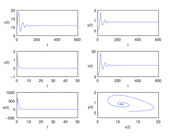
Figure 1. Simulation of system (3) for $\tau=1.6\in(\tau_{2},\tau_{1})$, showing convergence to the stable equilibrium $E_{s}$.

The notations and typical values of the parameters used in model (3) are given in Table 1.The precise value of $\tau$ is not obtained. But it is estimated that the value of $\tau$ is between $1.0\sim 1.5$ days [11]. Here, we choose $\tau$ as the bifurcation parameter.

For computer simulation, we set $\lambda=1$, $d=1/180$, $\alpha=\beta=1/260$, $a=0.5$, $b=2$, $p=q=3$, $k=80$, $c=1800$. Then, $\mathcal{R}_{0}=480/13e^{-0.5\tau}$ and $R_{1}=17$. The disease-free equilibrium $E_{0}$ is now given by

$$E_{0}=(180,\ 0,\ 0,\ 0,\ 0),$$

which is globally asymptotically stable for $\tau>\tau_{1}=7.2176734929$, i.e., $\mathcal{R}_{0}<1$. When $\tau<\tau_{1}$, $E_{0}$ becomes unstable and the single-infection equilibrium $E_{s}$ occurs, given by

$$E_{s}=(\frac{39}{8}e^{0.5\tau},\ 2e^{-0.5\tau}-\frac{13}{240},\ 0,\ \frac{160}{3}e^{-0.5\tau}-\frac{13}{9},\ 0),$$

which is globally asymptotically stable for $\tau_{1}>\tau>\tau_{2}=1.5512468048$. See Figure 1 for the simulations of system (3) when $\tau=1.6$.

Further decreasing $\tau$ to pass through the critical value $\tau_{2}$ will cause $E_{s}$ to lose its stability, giving rise to the double-infection equilibrium,

$$E_{d}=(\frac{180}{17},\ \frac{13}{15},\ \frac{8}{17}e^{-0.5\tau}-\frac{13}{60},\ \frac{208}{9},\ \frac{4800}{17}e^{-0.5\tau}-130).$$

The corresponding characteristic equation (14) at the above $E_{d}$ becomes

$$\begin{split}D(\xi)=&\ \xi^{5}+\Big{(}\frac{240}{221}e^{-0.5\tau}+\frac{1457}{180}\Big{)}\xi^{4}+(\frac{5828}{663}e^{-0.5\tau}+\frac{709}{45})\xi^{3}\\ &+\Big{(}\frac{15664}{663}e^{-0.5\tau}-\frac{19}{12}\Big{)}\xi^{2}+\Big{(}\frac{4796}{221}e^{-0.5\tau}-\frac{557}{60}\Big{)}\xi\\ &+\frac{24}{13}e^{-0.5\tau}-\frac{17}{20}-\Big{(}\frac{720}{221}\xi^{3}+\frac{212}{13}\xi^{2}+\frac{20}{221}\xi\Big{)}e^{-(\xi+0.5)\tau}=0.\end{split}$$ (19)

Let $R(\varpi,\tau)$ and $\varpi S(\varpi,\tau)$ be the real and imaginary parts of $D(i\varpi)\ (\varpi>0)$, yielding

$$\begin{split}R(\varpi,\tau)=&\ \Big{(}\frac{240}{221}e^{-0.5\tau}+\frac{1457}{180}\Big{)}\varpi^{4}-\Big{(}\frac{15664}{663}e^{-0.5\tau}-\frac{19}{12}\Big{)}\varpi^{2}+\frac{24}{13}e^{-0.5\tau}-\frac{17}{20}\\ &+\Big{(}\frac{720}{221}\varpi^{3}-\frac{20}{221}\varpi\Big{)}e^{-0.5\tau}\sin(\varpi\tau)+\frac{212}{13}\varpi^{2}e^{-0.5\tau}\cos(\varpi\tau),\\ S(\varpi,\tau)=&\ \varpi^{4}-\Big{(}\frac{5828}{663}e^{-0.5\tau}+\frac{709}{45}\Big{)}\varpi^{2}+\frac{4796}{221}e^{-0.5\tau}-\frac{557}{60}\\ &+\Big{(}\frac{720}{221}\varpi^{2}-\frac{20}{221}\Big{)}e^{-0.5\tau}\cos(\varpi\tau)-\frac{212}{13}\varpi e^{-0.5\tau}\sin(\varpi\tau),\end{split}$$

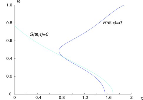
Figure 2. Plots of the curves $R(\varpi,\tau)=0$ and $S(\varpi,\tau)=0$ in the $\tau$-$\varpi$ plane with $(\varpi,\tau)\in[0,2.1]\times[0,2]$.

Solving the equations $R(\varpi,\tau)=0$ and $S(\varpi,\tau)=0$ by using the built-in command “fsolve” in Maple results in

$$(\tau_{3},\varpi_{3})=(0.8357983104,\ 0.4193565828).$$

Taking into account

$$\Big{(}\frac{720}{221}\varpi^{3}-\frac{20}{221}\varpi\Big{)}\sin(\varpi\tau)+\frac{212}{13}\varpi^{2}\cos(\varpi\tau)\geq-\frac{4}{221}\sqrt{\varpi^{2}(32400\varpi^{2}+1)(\varpi^{2}+25)},$$

we have $R(\varpi,\tau)\geq\widetilde{R}(\varpi)$, where

$$\begin{split}\widetilde{R}(\varpi)=&\ \frac{4}{221}\Big{[}60\varpi^{4}-\frac{3916}{3}\varpi^{2}+102-\varpi\sqrt{(32400\varpi^{2}+1)(\varpi^{2}+25)}\Big{]}e^{-0.5\tau}\\ &+\frac{1457}{180}\varpi^{4}+\frac{19}{12}\varpi^{2}-\frac{17}{20}.\end{split}$$

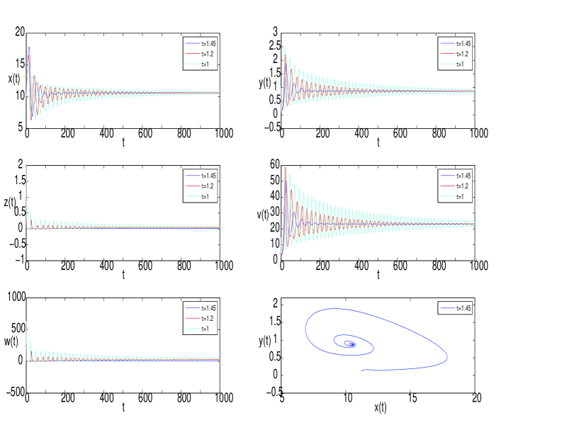
Figure 3. Simulation of system (3) for $\tau=1.45,\ 1.2$ and $1.0$, taken from the interval $\tau\in(\tau_{3},\tau_{2})$, showing convergence to the stable equilibrium $E_{d}$.

It can be shown that for any $\tau>0$, $\widetilde{R}(\varpi)>0$ if $\varpi>2.1$. Thus, there are no roots of $R(\varpi,\tau)=0$ for $\varpi>2.1$, implying that the curve $R(\varpi,\tau)=0$ in Figure 2 must be below the horizontal line $\varpi=2.1$ (not shown in Figure 2), and so $(\tau_{3},\varpi_{3})$ is the only intersection point. Given that all the roots of (19) continuously depend on $\tau$, it follows from Theorem 5.1 that $E_{d}$ is asymptotically stable when $\tau_{2}>\tau>\tau_{3}$. The simulations for $\tau=1.45,\ 1.2$ and $1.0$ are shown in Figure 3, from which we observe that all the components of a solution have more oscillating behaviors with larger amplitude, and they take longer time to converge to $E_{d}$ when $\tau$ is decreased from $\tau_{2}$ to $\tau_{3}$.

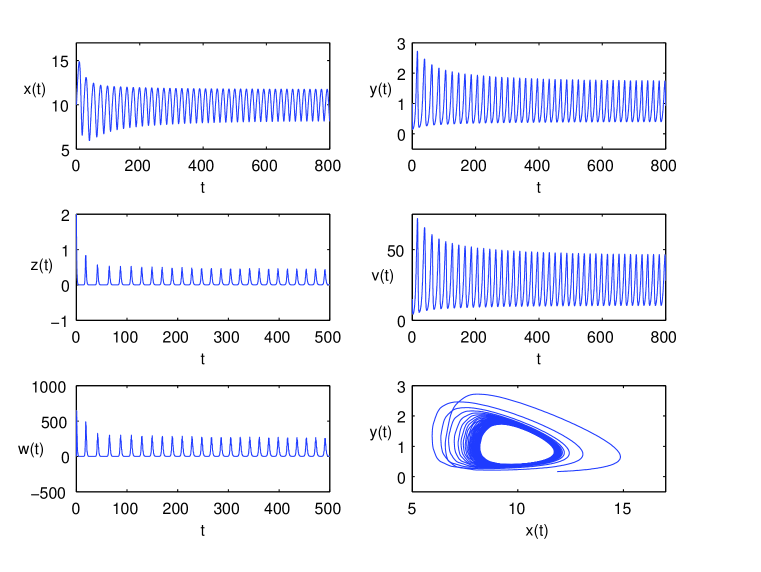
Figure 4. Simulation of system (3) for $\tau=0.8<\tau_{3}$, showing bifurcation to a stable limit cycle.

Finally, to consider possible Hopf bifurcation, first it is easy to see from Figure 2 that

$$S(\varpi,\tau)=0\quad\Longrightarrow\quad R(\varpi,\tau)<0,\quad{\rm for}\ \ \tau_{2}<\tau<\tau_{3},$$

indicating that condition (16) is satisfied. Moreover, the other two conditions also hold:

$$\left.\frac{\partial D(\xi,\tau)}{\partial\xi}\right|_{\xi=i\varpi_{3},\tau=\tau_{3}}=-9.8115344435+0.7314225159\,i\neq 0,$$

and

$$\left.{\rm Re}\Big{(}\frac{d\xi}{d\tau}\Big{)}\right|_{\xi=i\varpi_{3},\tau=\tau_{3}}=-0.0137073586<0.$$

Thus, the roots of (19) have positive real part when $\tau<\tau_{3}$, and (19) has a pair of purely imaginary roots at $\tau=\tau_{3}$, implying existence of a Hopf bifurcation. Therefore, we conclude that when $\tau_{2}>\tau>\tau_{3}$, the equilibrium solution $E_{d}$ is asymptotically stable. At the critical point, $\tau=\tau_{3}$, $E_{d}$ loses its stability through a Hopf bifurcation, giving rise to limit cycles. See the simulation shown in Figure 4. Further, the stability of limit cycles and the direction of bifurcations can be determined by using the center manifold theory and normal form theory for delay differential equations (e.g., see [16]). Detailed discussions on this part are out of the scope of this paper.

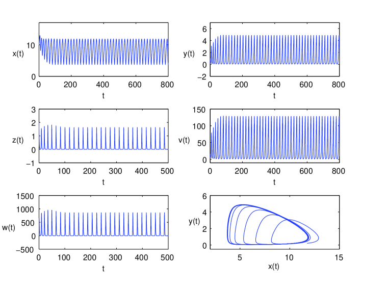
Figure 5. Simulation of system (3) for $\tau=0$, showing oscillating behaviour.

In order to demonstrate the importance of the delay to be included in the model, in the following we will compare the results obtained above to that given at $\tau=0$. It is easy to see that $\left.\mathcal{R}_{0}\right|_{\tau=0}=\frac{480}{13}>R_{1}=17$, and thus both the disease-free equilibrium, $E_{0}$, and the single-infection equilibrium, $E_{1}$, are unstable when $\tau=0$. To find the stability of the double-infection equilibrium, $E_{d}$, we set $\tau=0$ in (19) to obtain

$$D(\xi)=\xi^{5}+\frac{365197}{39780}\xi^{4}+\frac{211709}{9945}\xi^{3}+\frac{15209}{2652}\xi^{2}+\frac{163463}{13260}\xi+\frac{259}{260},$$

which yields a purely pair and three negative eigenvalues: $0.03214833+0.76348925\,i$, $-0.08306245$, $-3.91260798$, and $-5.24904353$, indicating that $E_{d}$ is also unstable. Therefore, at $\tau=0$, the system must exhibit oscillating behaviour, as shown in Figure 5. Comparing the results in this figure with that in Figure 4 shows that at $\tau=0$, the solution trajectory converges much fast to reach its steady-state value than that in Figure 4 for $\tau=0.8$ More importantly, it is noted that the amplitudes of the oscillations in Figure 5 is almost double of that in Figure 4 though their frequencies are almost not changed. The above observation shows that lack of even small delay in model (2) can cause significant quantitative changes in solutions. Moreover, for normal values of delay, the model (3) with delay can exhibit qualitatively different behaviour, compared with the model (2) without delay. For example, at $\tau=1.2$ days, which is within the normal range of delays $\tau\in(1.0,1.5)$ days [11], model (3) shows convergence to the stable double-infection equilibrium $E_{d}$, see Figure 3. At the marginal normal value $\tau=1.6$, model (3) gives the stable single-infection equilibrium $E_{s}$, see Figure 1. These significant qualitative changes due to existence of delay can not be observed from the model (2) without delay involved. This indeed suggests that the delay is a very important fact which should not be missed in model (2).

7. Conclusion and discussion

In this paper, we present a more realistic HIV-1 model of fighting a virus with another virus by adding delay to the model. The detailed analytic study has shown that the improved model with delay, like the model without delay, also has three equilibrium solutions: the disease-free equilibrium $E_{0}$, single-infection equilibrium $E_{s}$, and double-infection equilibrium $E_{d}$, and a series of bifurcations occur as the basic reproduction number, $\mathcal{R}_{0}$, is increased. It has shown that $E_{0}$ is globally asymptotically stable for $\mathcal{R}_{0}\in(0,1)$, and becomes unstable at the transcritical bifurcation point $\mathcal{R}_{0}=1$, and bifurcates into $E_{s}$, which is globally asymptotically stable for $\mathcal{R}_{0}\in(1,R_{1})$. $E_{s}$ loses its stability at the another transcritical bifurcation point $\mathcal{R}_{0}=R_{1}$, and asymptotically stable for $\mathcal{R}_{0}\in(R_{1},R_{h})$. Finally, $E_{d}$ becomes unstable at the Hopf critical point $\mathcal{R}_{0}=R_{h}$, and bifurcates into a family of limit cycles.

When the delay is chosen as the bifurcation parameter, it is shown that the delay plays an important role in determining the dynamic behaviour of the system. In the normal range of values, the delay may change the dynamic behaviour quantitatively, such as greatly reducing the amplitudes of oscillations, or even qualitatively changes the dynamical behaviour such as revoking oscillating solutions to equilibrium solutions. This indeed suggests that the delay is a very important fact which should not be missed in HIV-1 modelling.

In this paper, only Hopf bifurcation has been considered. It is interesting to know whether the model can exhibit double Hopf bifurcation if, besides the delay, one more system parameter is chosen as second bifurcation parameter. Another interesting question arises if we include another fact of delay to model (3), that is, the existence of virus production period for new virions to be produced within and released from the infected cells (see [10]). When this second delay is included, model (3) becomes

$$\begin{array}[]{cll}\dot{x}(t)&\!\!\!=\!\!\!&\lambda-dx(t)-\beta x(t)v(t),\\[1.42262pt] \dot{y}(t)&\!\!\!=\!\!\!&\beta e^{-a\tau_{1}}x(t-\tau_{1})v(t-\tau_{1})-ay(t)-\alpha w(t)y(t),\\[1.42262pt] \dot{z}(t)&\!\!\!=\!\!\!&\alpha w(t)y(t)-bz(t),\\[1.42262pt] \dot{v}(t)&\!\!\!=\!\!\!&ke^{-\tilde{a}\tau_{2}}y(t-\tau_{2})-pv(t),\\[1.42262pt] \dot{w}(t)&\!\!\!=\!\!\!&cz(t)-qw(t),\end{array}$$ (20)

where $\tau_{1}$ and $\tau_{2}$ represent the latent period and virus production period, respectively. Then for this model, future work includes the study on the dynamical behaviour and bifurcation patterns of the model, and how the two delays influence stability and bifurcations. More interestingly, with these two delays as bifurcation parameters, can the model exhibit double Hopf bifurcation? Studying these questions will help to well understand the impact of delays on dynamical behaviour of HIV-1 model.

Received xxxx 20xx; revised xxxx 20xx.

References

• [1] E. Beretta and Y. Kuang, Geometric stability switch criteria in delay differential systems with delay dependent parameters, SIAM J. Math. Anal., 33 (2002), 1144–1165.
• [2] S. Busenberg and K. Cooke, Vertically Transmitted Diseases: Models and Dynamics, Springer, New York, 1993.
• [3] F. Gantmacher, The Theory of Matrices, Vol. 2, Chelsea, New York,1959.
• [4] J. Hale and S. Verduyn Lunel, Introduction to Functional Differential Equations, Springer-Verlag, New York, 1993.
• [5] B. D. Hassard, N. D. Kazarinoff and Y.-H. Wan, Theory and applications of Hopf bifurcation, Cambridge University Press, Cambridge, 1981.
• [6] X. Jiang, P. Yu, Z. Yuan and X. Zou, Dynamics of an HIV-1 therapy model of fighting a virus with another virus, Journal of Biological Dynamics, 3 (2009), 387–409.
• [7] T. Kajiwara, T. Saraki and Y. Takeuchi, Construction of lyapunov functionals for delay differential equations in virology and epidemiology, Nonlinear Analysis: Real World Applications, 13 (2012), 1802–1826.
• [8] J. LaSalle, The Stability of Dynamical Systems, SIAM, Philadelphia, 1976.
• [9] C. Michie, A. McLean, C. Alcock and P. Beverly, Lifespan of human lymphocyte subsets defined by cd45 isoforms, Nature, 360 (1992), 264–265.
• [10] J. Mittler, B. Sulzer, A. Neumann and A. Perelson, Influence of delayed virus production on viral dynamics in HIV-1 infected patients, Math.Biosci, 152 (1998), 143–163.
• [11] P. W. Nelson, J. D. Murray and A. S. Perelson, A model of HIV-1 pathogenesis that includes an intracellular delay, Mathematical Biosciences, 163 (2000), 201–215.
• [12] G. Nolan, Harnessing viral devices as pharmaceuticals: fighting HIV-1s fire with fire, Cell, 90 (1997), 821–824.
• [13] T. Revilla and G. García-Ramos, Fighting a virus with a virus: a dynamic model for HIV-1 therapy, Math. Biosci., 185 (2003), 191–203.
• [14] H. L. Smith, Monotone Dynamical Systems: An Introduction to the Theory of Competitive and Cooperative Systems, Mathematical Surveys and Monographs, Vol. 41 (American Mathematical Socienty, Providence, RI, 1995.
• [15] E. Wagner, M. Hewlett, Basic Virology, Blackwell, New York, 1999.
• [16] P. Yu, Y. Ding, W. Jiang, Equivalence of MTS method and CMR method for delay differential equations associated with semisimple singularity, Int. J. Bifurcation and Chaos, 24 (2014), 1450003 (49 pages).
• [17] H. Zhu and X. Zou, Impact of delays in cell infection and virus production on HIV-1 dynamics, Math. Medic. Bio., 25 (2008), 99–112.
• [18] P. Yu and X. Zou, Bifurcation analysis on an HIV-1 Model with constant injection of recombinant, Int. J. Bifurcation and Chaos, 22(3) (2012), 1250062 (21 pages).
• [19] H. Zhu and X. Zou, Dynamics of a HIV-1 infection model with cell-mediated immune response and intracellular delay, Disc. Cont. Dyan. Syst. B., 12 (2009), 511–524.