Localised auxin peaks in concentration-based transport models of the shoot apical meristem

Abstract

We study the formation of auxin peaks in a generic class of concentration-based auxin transport models, posed on static plant tissues. Using standard asymptotic analysis we prove that, on bounded domains, auxin peaks are not formed via a Turing instability in the active transport parameter, but via simple corrections to the homogeneous steady state. When the active transport is small, the geometry of the tissue encodes the peaks’ amplitude and location: peaks arise where cells have fewer neighbours, that is, at the boundary of the domain. We test our theory and perform numerical bifurcation analysis on two models which are known to generate auxin patterns for biologically plausible parameter values. In the same parameter regimes, we find that realistic tissues are capable of generating a multitude of stationary patterns, with a variable number of auxin peaks, that can be selected by different initial conditions or by quasi-static changes in the active transport parameter. The competition between active transport and production rate determines whether peaks remain localised or cover the entire domain. We relate the occurrence of localised patterns to a snaking bifurcation structure, which is known to arise in a wide variety of nonlinear media but has not yet been reported in plant models.

Keywords: auxin transport model, auxin patterns, localised patterns, snaking, numerical bifurcation analysis

1 Introduction

The hormone auxin plays a crucial role in plant development [1, 2, 3, 4], yet the mechanisms through which it accumulates in certain cells and interacts with cell growth mechanisms remain largely unclear. The patterns formed during the growth of a plant are controlled by the local auxin concentration. For example, it is known that the distribution of auxin maxima in the shoot apex gives rise to the formation of primordia [5, 6, 7, 8, 10, 11]. Similarly, the distribution of auxin in the root tip coordinates cell division and cell expansion [12, 13]. In models of root hair initiation, intra-cellular levels and gradients of auxin concentration influence the localisation of G-proteins, which in turn promote hair formation [14]. In addition, it is known that the distribution of auxin in the leaf primordia mediates vascular patterning [1]. In recent years, many aspects of the molecular basis of these mechanisms have been unraveled and mathematical models of auxin transport have been proposed to explain growth and development [15, 16, 17, 18].

Computer simulations are often used to compare the model output with observed data such as auxin distribution, venation patterns, growth or development. At cellular level, carriers such as PIN-FORMED (PIN) proteins, which are localised in the cell membrane, determine the rate and direction of auxin transport. The coordinated activity of many cells can create peaks of auxin that drive differentiation and growth. Various models that implement and refine these ideas have been proposed [5, 6, 7, 12, 19, 20, 21]. Such models differ primarily in the specifics of the transport and the coupling to the cell growth and division, but a common feature is that they generate spatially-extended patterns of auxin concentration, which have also been observed experimentally.

Existing transport models can be classified into two main categories, flux-based and concentration-based, depending on how auxin influences the localization of transport mediators (PINs) to form patterns. In flux-based models, first proposed in [22], the polarization depends on the net auxin flux between neighbouring cells: the higher the net flux towards the neighbours, the more PIN will accumulate at the membrane, and changes in the PIN distribution determine changes in auxin fluxes. By contrast, in concentration-based models it is assumed that the PIN accumulation on the membrane is caused by differences in auxin concentration between neighbouring cells. This type of models was introduced in [5] and [7]. For other reviews on flux- and concentration-based models we refer the reader to [24, 25, 26, 27].

In the models mentioned above, patterns are found by direct numerical simulation, upon choosing control parameters within a plausible biological range. However, there is still a large uncertainty on many of the parameter values which are often approximated [28, 29], adopted from different systems [30] or estimated with large error margins [31]. Furthermore, it is unclear what is the effect of systematic parameter variations on the generated patterns and how this relates to the behaviour of the biological system: understanding the formation of auxin peaks from a dynamical system standpoint is still an open problem, therefore a mathematical exploration of the parameter variations may generate new, experimentally testable hypotheses, thereby gaining insight into pattern formation mechanisms [1, 10, 32].

In spite of the uncertainty on experimental parameters, it is believed that active transport is a key player in auxin patterning [29]. Transport models posses an inherent time-scale separation: the growth hormone dynamics involve short time scales (of the order of seconds) [53], while changes in cellular shapes and proliferation of new cells occur on much slower time scales (hours or days) [54]. In order to determine the distribution of auxin in the plant, it is then possible to concentrate on the fast time scale of the hormone transport, assume a static cell structure and study the plant tissue as a dynamical system, subject to variations in the active transport parameter.

In this paper we perform such exploration on concentration-based auxin models, which are studied using standard bifurcation analysis techniques [33]. In particular, we find steady states of the system and explore their dependence upon control parameters, investigating how patterns lose or gain stability in response to parameter changes. The aim is to predict qualitatively the distribution patterns that can occur for a certain parameter range and to understand transitions between different types of patterns.

At present, only a few papers regard transport models as dynamical systems: among them, Reference [23] stands out for being a systematic analysis of flux- and concentration-based models, whose auxin patterns are studied by considering local interactions between cells. In the present paper, we take the analysis one step further, by finding steady states simultaneously in the whole tissue, and by studying the important effects of its boundedness on the auxin patterns.

The main result of our analysis is that, in a large class of concentration-based models posed on finite tissues, peaks do not arise from an instability of the homogeneous steady state, as it was previously reported for unbounded tissues [5, 7, 36, 37]: on regular bounded domains, the geometry of the tissue drives the formation of small auxin peaks, which nucleate without instabilities near the boundary.

Further, we investigate the effects of changes in the active transport coefficient, in the diffusivity coefficient and in the auxin production coefficient for two specific examples: the concentration-based model proposed by Smith et al.[5] and a more recent modification studied by Chitwood et al.[34]. In these systems the localised peaks, determined analytically for small values of the active transport coefficient, persist also for moderate and large values of this control parameter. We found that, owing to their boundedness, realistic tissues can select from a multitude of patterned configurations, characterised by a variable number of localised peaks and organised in a characteristic snaking bifurcation diagram.

Snaking bifurcation diagrams are commonly found for localised states  arising in (systems of) nonlinear partial differential equations posed in one [38, 39, 40, 41, 42, 43], two [44, 45] and three [46, 47] spatial dimensions, as well as in discrete [48] and nonlocal systems [49, 50, 51, 52]. However, this mechanism has never been reported for auxin models: solutions with localised peaks undergo a series of saddle-node bifurcations, giving rise to a hierarchy of steady states with an increasing number of bumps. A direct consequence of this mechanism is that the resulting patterns are robust against changes in the transport parameter and other control parameters as found, for instance, by Sahlin et al. [36]. We argue that this mechanism could be a robust feature in several other types of concentration-based auxin models.

The paper is structured as follows: in Section 2 we summarise our working hypotheses and describe the main results of the paper; in Section 3.1 we present our calculations for a simple 1D tissue, giving a primer on bifurcation analysis for auxin models; in Section 3.2 we generalise our results to 2D tissues, which are further discussed in Section 4; finally, we provide a more formal presentation of our general asymptotic results in Section 5.

2 Mathematical formulation and summary of the main results

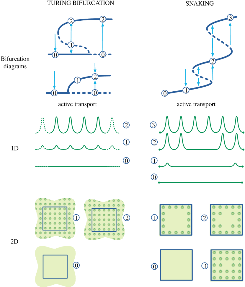
Fig. 1: Two mechanisms for the formation of spots, explained with bifurcation diagrams (top) and representative patterns in 1D (centre) and 2D (bottom). Turing bifurcation (left): on unbounded domains, or bounded domains with periodic boundary conditions, the homogeneous state (0) is attracting for low values of the active transport parameter $T$ (a blue arrow indicates time evolution); when $T$ is increased above a critical value, the flat state becomes unstable and the system evolves towards a fully patterned state (2); states with low auxin peaks (1) may be attracting or repelling, depending on the bifurcation type. Snaking mechanism (right): on bounded domains with free boundary conditions, the flat state (0) exists only for $T=0$; upon increasing $T$, we find an attracting state with low auxin peaks at the boundary (1), followed by several other attracting states with variable number of peaks (2, 3); the tissue is able to select from different patterns, depending on the initial condition and on the value of $T$.

We begin by giving a generic definition of concentration-based models, and a summary of the main results of the paper. In concentration-based models, cells are identified with an index $i\in\{1,\ldots,n\}$ and to each cell it is associated a set of neighbours $\mathcal{N}_{i}$, containing $|\mathcal{N}_{i}|$ neighbours, and a vector of $m$ time-dependent state variables $\bm{y}_{i}(t)$. For instance, $\bm{y}_{i}$ may contain the auxin concentration ($m=1$) or both auxin and PIN-FORMED1 concentrations ($m=2$). Generically, the rate of change of the concentrations is expressed as a balance between production and decay within the cell, diffusion towards neighbouring cells and active transport, hence we study generic concentration-based auxin models of the form

$$\dot{\bm{y}}_{i}=\bm{\pi}(\bm{y}_{i})-\bm{\delta}(\bm{y}_{i})+\bm{D}\sum_{j\in\mathcal{N}_{i}}(\bm{y}_{j}-\bm{y}_{i})+T\sum_{j\in\mathcal{N}_{i}}\bm{\nu}_{ji}(\bm{y}_{1},\ldots,\bm{y}_{n})-\bm{\nu}_{ij}(\bm{y}_{1},\ldots,\bm{y}_{n}),$$ (1)

where $\bm{\pi},\bm{\delta}$, are the production and decay functions, respectively, $\bm{D}$ is a diffusion matrix, $T$ is the active transport parameter and $\bm{\nu}_{ij}$ are the active transport functions. In this paper we concentrate on the fast time scale of hormone transport and hence consider plant organs as static cell structures, so the number of cells $n$ remains constant in time. We make two key assumptions:

Hypothesis 1 (Regular domains).

Cells are arranged in a regular domain, that is, they have all the same shape and size and they tessellate the tissue. We do not make any assumption on the dimensionality of the domain.

Hypothesis 2 (Active transport functions).

The active transport functions can be expressed as

$$(\bm{\nu}_{ij})_{l}=\psi_{l}(\bm{y}_{i},\bm{y}_{j})\frac{\varphi_{l}(\bm{y}_{j})}{\sum_{k\in\mathcal{N}_{i}}\varphi_{l}(\bm{y}_{k})},\quad\textrm{for $l=1,\ldots,m$},$$ (2)

where the functions $\psi_{l}$, $\varphi_{l}$ depend on the model choices.

Hypothesis 2 is a factorisation of the active transport functions that is met by several models in literature [5, 7, 35, 31, 34]: active transport between cell $i$ and $j$ is influenced by the respective concentrations $\bm{y}_{i}$ and $\bm{y}_{j}$, but also by concentrations in the neighbours of cell $i$. In Section 2.1 we introduce examples of concrete models satisfying Hypothesis 2 and in Section 5 we derive explicit expressions for the corresponding functions $\psi_{l}$, $\varphi_{l}$.

It is established in literature that concentration-based models are capable of reproducing auxin patterns that are found in SAM experiments [5, 7, 6, 58, 34, 36], for biologically realistic values of the transport parameters. In this paper we will address the following questions: What type of patterns are generated by the class of models described above? Do they all predict the occurrence of auxin peaks? What are the instabilities that lead to the formation of auxin peaks? Are auxin patterns robust to changes in the control parameters and initial conditions?

These question have been partially addressed in previous papers [5, 7, 34, 36, 6, 56, 23], where analytical results have been obtained only for particular models and only for regular domains without boundaries, where all cells have the same number of neighbours. In such domains a homogeneous steady state $\bm{y}_{i}=\bm{y}^{*}$, satisfying the balancing condition $\bm{\pi}(\bm{y}_{i})=\bm{\delta}(\bm{y}_{i})$, is known to exist for all values of $T$ [5, 6, 7, 34, 36, 56, 37]. In domains without boundaries, the formation of peaks has been explained in terms of a Turing bifurcation in the active transport parameter (see Figure 1): peaks are formed all at once as $T$ is varied, and they derive from an instability of the homogeneous steady state. From a dynamical system viewpoint, however, we expect that boundary conditions and finite domain sizes affect the formation and selection of auxin patterns. The main result of our investigation is that the mechanism for the formation of peaks is radically different in tissues of finite size, and in particular:

Result 1 (Homogeneous steady states).

In finite domains, concentration-based models (1) satisfying Hypotheses 1–2 support a homogeneous equilibrium $\bm{y}_{i}=\bm{y}^{*}$ for $T=0$ but, generically, this homogeneous state is not present when $T\neq 0$. This result is a direct consequence of the geometry of the domain: an inspection of Equation (2) shows that the active transport terms $\bm{\nu}_{ij}$ contain a nested sum over the neighbours of the cell $i$ and, in a finite domain, the number of neighbours varies from cell to cell, namely cells at the boundary of the regular tissue have fewer neighbours than cells in the interior; consequently, $\bm{\nu}_{ij}-\bm{\nu}_{ji}$ is generally different from $\mathbf{0}$ at the boundary, even when $\bm{y}_{i}=\bm{y}^{*}$. The conclusion is that, on finite domains, peaks can not form with a Turing bifurcation, since the homogeneous steady state exists for $T=0$, but not for $T\neq 0$ (however small). For regular domains where the number of neighbours is the same for all cells, the Turing mechanism is still possible. In addition, a Turing bifurcation is also possible in any domain, provided that $T=0$ and diffusion is used as a bifurcation parameter. In this regime, however, the active transport is absent and the tissue is a standard medium with reaction-diffusion mechanisms, which is not a biologically valid hypothesis for auxin models.

Result 2 (Origin of auxin peaks).

To understand how peaks are formed from the homogeneous state we study the case of small active transport coefficients. For $0<T\ll 1$ and in the absence of passive transport, $\bm{D}=\mathbf{0}$, the models above generate steady states with small peaks. Such states take the form

$$\bm{y}_{i}=\bm{y}^{*}+T\xi_{i}\big{[}\bm{\pi}^{\prime}(\bm{y}^{*})-\bm{\delta}^{\prime}(\bm{y}^{*})\big{]}^{-1}\bm{\psi}(\bm{y}^{*},\bm{y}^{*})+\mathcal{O}(T^{2})$$ (3)

where the coefficients $\xi_{i}$ depend on the number of neighbours at distance 2 from the $i$th cell, namely

$$\xi_{i}=1-\sum_{j\in\mathcal{N}_{i}}\frac{1}{|\mathcal{N}_{j}|}.$$

Equation (3) predicts that peaks are formed as small perturbations of the homogeneous steady state (see Figure 1). The amplitude of small peaks is proportional to $T$ and $\xi_{i}$. Importantly, $\xi_{i}=0$ in the interior of regular domains, therefore peaks localise at the boundary and without bifurcations, as opposed to the Turing scenario where they form everywhere owing to an instability of $\bm{y}^{*}$: the mechanism on finite domains is purely geometric, as the location of the peaks is determined by the factors $\xi_{i}$.

Result 3 (Effect of passive transport).

For small active transport and at the presence of passive transport, $\bm{D}\neq\mathbf{0}$, we still obtain solutions with localised peaks, similar to the case discussed above. The location of the peaks depends again on $\xi_{1},\ldots,\xi_{n}$.

Remark 2.1 (Applicability of analytical results).

Results 1–3 are valid for generic models of the form (1), provided they satisfy Hypotheses 1–2. In particular, these results are valid for regular cellular arrays in any spatial dimension. The main implication of this result is that a wide class of concentration-based models are able to generate spontaneously auxin peaks in various geometries, irrespective of the model specifics. A similar derivation can be done for irregular domains, albeit the coefficients $\xi_{i}$ depend in this case on the local cellular volumes as well as the number of neighbours.

The analytical theory described above, which is presented in more detail in Section 5, is valid only for small values of the active transport coefficient and does not explain the formation of peaks in the interior of the domain [6, 36, 9]. While it is difficult to make general analytical predictions for larger values of $T$, it is possible to explore the solution landscape of specific models via numerical methods. We investigated regular domains in two concrete models by Smith et al. [5] and Chitwood et al. [34] (henceforth called the Smith model and the Chitwood model, respectively) which satisfy Hypotheses 1–2 and will be described in detail in Section 2.1. Our computations confirm the theoretical Results 1–3 and provide numerical evidence for the following conclusions:

Result 4 (Formation of stable auxin spots in the interior).

As the active transport rises, the two models by Smith and Chitwood predict the formation of peaks in the interior. Peaks are formed progressively, from the boundary towards the interior via saddle-node bifurcations, with a characteristic snaking bifurcation diagram. From a biological perspective, this means that the tissue can form peaks that are robust with respect to changes in the control parameters. In addition, the tissue is capable of selecting from a variety of auxin patterns, with a variable number of spots, depending on the initial conditions and on the value of the auxin transport parameter $T$ (see Figure 1).

Result 5 (Robustness of the snaking mechanism).

The scenario above is robust to perturbations to secondary parameters, that is, solutions with localised peaks at the boundary should be observable in experiments for which the two models are applicable, if the active transport is inhibited with respect to passive transport.

Furthermore, in numerical calculations we are able to violate Hypotheses 1–2 and see how this affects our results. An important conclusion is the following:

Result 6 (Irregular domains).

When the Smith and the Chitwood models are posed on irregular domains, the bifurcation structure presented above persists. Auxin peaks are formed progressively via saddle-node bifurcations, albeit they may in principle nucleate in the interior of the domain before the boundary is filled. Furthermore, this scenario is robust to changes in secondary parameters, so Result 5 is still valid on irregular domains for both models.

2.1 Two models of auxin transport

We now present two models that will be analysed in detail using the asymptotic theory of Section 5 and numerical simulations. As a first example we consider the Smith model [5], which features 2 state variables per cell, namely the indole-3-acetic acid (IAA) concentration, $a_{i}(t)$, and the PIN-FORMED1 (PIN1) amount, $p_{i}(t)$. The model features IAA production, decay, active and passive transport terms, whereas for PIN1 only production and decay are included. This results in the following set of coupled nonlinear ODEs

$$\begin{split}\frac{da_{i}}{dt}=&\frac{\rho_{\textnormal{{\tiny IAA}}}}{1+\kappa_{\textnormal{{\tiny IAA}}}a_{i}}-\mu_{\textnormal{{\tiny IAA}}}a_{i}+\frac{D}{V_{i}}\sum_{j\in\mathcal{N}_{i}}l_{ij}\big{(}a_{j}-a_{i}\big{)}\\ &+\frac{T}{V_{i}}\sum_{j\in\mathcal{N}_{i}}\Bigg{[}P_{ji}(\bm{a},\bm{p})\frac{a_{j}^{2}}{1+\kappa_{T}a_{i}^{2}}-P_{ij}(\bm{a},\bm{p})\frac{a_{i}^{2}}{1+\kappa_{T}a_{j}^{2}}\Bigg{]},\end{split}$$ (4)

$$\frac{dp_{i}}{dt}= \frac{\rho_{\textnormal{{\tiny PIN}}_{0}}+\rho_{\textnormal{{\tiny PIN}}}a_{i}}{1+\kappa_{\textnormal{{\tiny PIN}}}p_{i}}-\mu_{\textnormal{{\tiny PIN}}}p_{i},$$ (5)

for $i=1,\ldots,n$. In this model $D$ is a diffusion coefficient, $V_{i}$ is the cellular volume, $l_{ij}=S_{ij}/(W_{i}+W_{j})$ is the ratio between the contact area $S_{ij}$ of the adjacent cells $i$ and $j$, and the sum of the corresponding cellular wall thicknesses $W_{i}$ and $W_{j}$. In addition, $T$ is the active transport coefficient and $P_{ij}$ is the number of PIN1 proteins on the cellular membrane of cell $i$ facing cell $j$,

$$P_{ij}(\bm{a},\bm{p})=p_{i}\frac{l_{ij}\exp{(c_{1}a_{j})}}{\sum_{k\in\mathcal{N}_{i}}l_{ik}\exp{(c_{1}a_{k})}}.$$ (6)

The Smith model posed on a regular domain satisfies Hypotheses 1–2 in Section 2 and the reader can find explicit expressions for the functions $\varphi_{l}$, $\psi_{l}$ in Section 5.1.2. More details on the model and simulations of realistic phyllotactic patterns can be found in [5].

The second concentration-based transport model that will be studied below is the more recent Chitwood model [34]. This modification of the Smith model is able to produce stable spiral phyllotactic patterns once cell division is included. The system also features 2 variables per cell, the IAA concentration and the PIN1 amount, and it is given by the following set of coupled nonlinear ODEs

$$\begin{split}\frac{da_{i}}{dt}=&\frac{\rho_{\textnormal{{\tiny IAA}}}}{1+\kappa_{\textnormal{{\tiny IAA}}}a_{i}}-\mu_{\textnormal{{\tiny IAA}}}a_{i}+\frac{D}{V_{i}}\sum_{j\in\mathcal{N}_{i}}l_{ij}\big{(}a_{j}-a_{i}\big{)}\\ &+\frac{T}{V_{i}}\sum_{j\in\mathcal{N}_{i}}\Bigg{[}P_{ji}(\bm{a},\bm{p})\frac{\exp{(c_{2}a_{j})}-1}{\exp{(c_{2}a_{i})}}-P_{ij}(\bm{a},\bm{p})\frac{\exp{(c_{2}a_{i})}-1}{\exp{(c_{2}a_{j})}}\Bigg{]},\end{split}$$ (7)

$$\frac{dp_{i}}{dt}= \frac{\rho_{\textnormal{{\tiny PIN}}_{0}}+\rho_{\textnormal{{\tiny PIN}}}a_{i}}{1+\kappa_{\textnormal{{\tiny PIN}}}p_{i}}-\mu_{\textnormal{{\tiny PIN}}}p_{i},$$ (8)

for $i=1,\ldots,n$, where $P_{ij}$ are given by (6) and the only new parameter, $c_{2}$, controls the exponential transport. The Chitwood model posed on a regular domain also satisfies Hypotheses 1–2, as shown in Section 5.1.2.

In the reminder of the paper we shall fix most parameters in the Smith and the Chitwood models, and we will examine variations in the active transport parameter $T$, auxin diffusion coefficient $D$ and auxin production coefficient $\rho_{\textnormal{{\tiny IAA}}}$. In Table 1 we report a brief description of parameters for both models, together with characteristic values and units, which are taken from [5, 34].

Table 1: Control parameters for the Smith and Chitwood models (parameter values are taken from [5] and [34]). We examine variations in $T$, $D$ and $\rho_{{}_{\textnormal{{\tiny IAA}}}}$, for which we report a range of values in the second part of the table.

Symbol	Description	Domain	Value		Unit
			Smith et al.	Chitwood et al.
$c_{1}$	PIN distribution		$1.099$	$1.099$	1/$\mu$M
$\kappa_{{}_{\textnormal{{\tiny PIN}}}}$	PIN saturation		$1$	$1$	1/$\mu$M
$\kappa_{T}$	Transport saturation		$1$
$c_{2}$	Exponential transport	2D reg.		$0.588$	1/$\mu$M
		2D irreg.		$0.405$	1/$\mu$M
$\kappa_{{}_{\textnormal{{\tiny IAA}}}}$	IAA saturation		$1$	$1$	1/$\mu$M
$\rho_{{}_{\textnormal{{\tiny PIN}}_{0}}}$	PIN base production		$0$	$0$	$\mu$M/h
$\rho_{{}_{\textnormal{{\tiny PIN}}}}$	PIN production		$1$	$1$	1/h
$\mu_{{}_{\textnormal{{\tiny PIN}}}}$	PIN decay		$0.1$	$0.1$	1/h
$\mu_{{}_{\textnormal{{\tiny IAA}}}}$	IAA decay		$0.1$	$0.1$	1/h
$\rho_{{}_{\textnormal{{\tiny IAA}}}}$	IAA production		$\left[0.3,1.5\right]$	$\left[0.7,2.0\right]$	$\mu$M/h
$D$	IAA diffusion		$\left[0,1\right]$	$\left[0,1\right]$	$\mu$m2/h
$T$	IAA transport coefficient	1D reg.	$\left[0,6\right]$		$\mu$m3/h
		2D reg.	$\left[0,2\right]$	$\left[0,2.5\right]$	$\mu$m3/h
		2D irreg.	$\left[0,120\right]$	$\left[0,95\right]$	$\mu$m3/h

Remark 2.2 (Comparison with experimental parameters).

The model equations 4–8 show that the transport parameters $T$ and $D$ are scaled by the cellular volumes $V_{i}$: comparisons to experimental parameters and other computer simulations available in literature should be based on the ratios $T/V_{i}$ and $D/V_{i}$. Through these ratios we implicitly specify $T/D$, so as to account for competition between active and passive transports.

Remark 2.3 (Tissue types).

We model 3 plant tissues: identical cubic cells arranged on a line of finite length (here and henceforth, 1D regular), identical hexagonal prismic cells tessellating a finite square (2D regular) and irregular prismic cells tessellating an almost-circular domain (2D irregular, taken from Merks et al. [55]). We stress that the nomenclature 1D and 2D refers to the domain, not the cells, which are assumed to have consistently assigned volumes and contact areas. We note that cellular volumes and contact areas may change between different domains (see also Remark 2.2).

3 Results

3.1 A primer on the formation of auxin peaks - a 1D regular tissue

Fig. 2: Approximate solution pattern in the 1D regular tissue. Top: geometry of a one-dimensional cellular array of identical cells; there exist cells to the left of $i=1$, but the next flux with cell $1$ is 0; at $i=n$ we have a physical boundary, therefore no cells exist to the right of cell $n$ and $\mathcal{N}_{n}=n-1$. Bottom: predicted approximate solution pattern $a^{*}+T\alpha_{i}$ in the proximity of the boundary $i=n$ for the Smith model with $n=150$ and various values of the diffusion coefficient. Parameters: $T=3\cdot 10^{-5}\mu\textrm{m}^{3}/\textrm{h}$, $D=1\,\mu\textrm{m}^{2}/\textrm{h}$, $\rho_{\textnormal{{\tiny IAA}}}=0.85\,\mu\textrm{M}/\textrm{h}$ other parameters as in Table 1.

In this section, we present in detail Results 1–5 for the Smith model posed on a 1D regular tissue, which is represented in Figure 2. The tissue consists of a file of $n$ identical cubic cells with volume $V=1\mu\textrm{m}^{3}$ and $l_{ij}=1\,\mu\textrm{m}$. We assume that there exist cells to the left of cell $1$ and that the net proximal flux is zero, hence we prescribe Neumann boundary conditions at $i=1$. We impose that there are no cells to the right of cell $n$, so we use a free boundary condition at $i=n$ by setting $\mathcal{N}_{n}=n-1$. In this geometry, the tissue has a physical boundary only at $i=n$, as illustrated in Figure 2, so each cell has $2$ neighbours, except cell $n$, which has only $1$ neighbour. This geometry (with periodic boundary conditions) has been studied in other auxin-patterning simulations: it was used in reference [56] as an approximation of a root tissue and in reference [59] to model part of a leaf, between the midvein and the margin. In this paper, we use this geometry only as a primer to illustrate how the asymptotic and numerical calculations are used to predict the formation of auxin spots in concentration-based models. While the focus is on the Smith model, several of the results presented in this section, are valid in more general models and spatial configurations (we refer the reader to Remark 2.1 and the whole Section 2 for further comments on the generality of these results).

3.1.1 From homogeneous to patterned solutions

The Smith model posed on a regular domain satisfies Hypotheses 1–2 (as shown in Section 5.1.2), so we can apply the asymptotic theory in Section 5 (in particular, Lemma 5.1). On an unbounded array (or on a bounded array with periodic boundary conditions) every cell has the same number of neighbours, therefore the model admits the following homogeneous steady state

$$a_{i}=a^{*}=\frac{-1+\sqrt{1+4\kappa_{\textnormal{{\tiny IAA}}}\rho_{\textnormal{{\tiny IAA}}}/\mu_{\textnormal{{\tiny IAA}}}}}{2\kappa_{\textnormal{{\tiny IAA}}}},$$ (9)

$$p_{i}=p^{*}=\frac{-1+\sqrt{1+4\kappa_{\textnormal{{\tiny PIN}}}(\rho_{\textnormal{{\tiny PIN}}_{0}}+\rho_{\textnormal{{\tiny PIN}}}a^{*})/\mu_{\textnormal{{\tiny PIN}}}}}{2\kappa_{\textnormal{{\tiny PIN}}}},$$

for $i=1,\ldots n$. However the 1D regular domain considered here is finite, so the homogeneous solution exists only for $T=0\;\mu\textrm{m}^{3}/\textrm{h}$, as for positive $T$ the sums in the transport term in (4) do not vanish in general (Result 1). For $D=0\,\mu\textrm{m}^{2}/\textrm{h}$ and $T\ll 1\,\mu\textrm{m}^{3}/\textrm{h}$, Lemma 5.1 shows the existence of patterns in the form of small deviations from the homogeneous steady state (see Section 5.1.2 for a full derivation)

$$a_{i} =\begin{cases}a^{*}&\text{for $i=1\ldots n-2$,}\\[10.00002pt] a^{*}+T\dfrac{p^{*}}{2V}\bigg{[}\dfrac{\rho_{\textnormal{{\tiny IAA}}}\kappa_{\textnormal{{\tiny IAA}}}}{1+\kappa_{\textnormal{{\tiny IAA}}}(a^{*})^{2}}+\mu_{\textnormal{{\tiny IAA}}}\bigg{]}^{-1}\dfrac{(a^{*})^{2}}{1+\kappa_{T}(a^{*})^{2}}&\text{for $i=n-1$,}\\[10.00002pt] a^{*}-T\dfrac{p^{*}}{2V}\bigg{[}\dfrac{\rho_{\textnormal{{\tiny IAA}}}\kappa_{\textnormal{{\tiny IAA}}}}{1+\kappa_{\textnormal{{\tiny IAA}}}(a^{*})^{2}}+\mu_{\textnormal{{\tiny IAA}}}\bigg{]}^{-1}\dfrac{(a^{*})^{2}}{1+\kappa_{T}(a^{*})^{2}}&\text{for $i=n$.}\end{cases}$$ (10)

$$p_{i} =\begin{cases}p^{*}&\text{for $i=1,\ldots,n-2$},\\ p^{*}+\left[\dfrac{(\rho_{\textnormal{{\tiny PIN}}_{0}}+\rho_{\textnormal{{\tiny PIN}}}a^{*})\kappa_{\textnormal{{\tiny PIN}}}}{(1+\kappa_{\textnormal{{\tiny PIN}}}p^{*})^{2}}+\mu_{\textnormal{{\tiny PIN}}}\right]^{-1}\!\!\!\dfrac{\rho_{\textnormal{{\tiny PIN}}}}{1+\kappa_{\textnormal{{\tiny PIN}}}p^{*}}(a_{i}-a^{*})&\text{for $i=n-1$},\\ p^{*}-\left[\dfrac{(\rho_{\textnormal{{\tiny PIN}}_{0}}+\rho_{\textnormal{{\tiny PIN}}}a^{*})\kappa_{\textnormal{{\tiny PIN}}}}{(1+\kappa_{\textnormal{{\tiny PIN}}}p^{*})^{2}}+\mu_{\textnormal{{\tiny PIN}}}\right]^{-1}\!\!\!\dfrac{\rho_{\textnormal{{\tiny PIN}}}}{1+\kappa_{\textnormal{{\tiny PIN}}}p^{*}}(a_{i}-a^{*})&\text{for $i=n$}.\end{cases}$$

The equations above predict that, for infinitesimal values of the transport coefficient $T$, the perturbed solution coincides with the homogeneous solution, except for a small peak at cell $n-1$ and a small dip at cell $n$ (see also bold curve in Figure 2). In other words, peaks are present where the number of neighbours differs from the number of neighbours in the unbounded domain, that is, where the sum in the active transport in Equation (4) is nonzero (Result 2). The analysis above applies also in the limit of slow dynamics of the PIN1 proteins: upon assuming $p$ constant and homogeneous in the tissue, we find that $a_{i}$ is as in Equation 10, with $p^{*}$ replaced by $p$ (see Section 5.1.1 for details).

We have thus established that, in regular domains, a small auxin transport coefficient $T$ elicit low auxin peaks. Such correlation was previously reported in numerical experiments on various models [7, 36] and we now provide a mathematical explanation of this phenomenon.

Asymptotic calculations can also be carried out in the presence of diffusion ($D\neq 0$), leading to a linear system for the perturbations. In Section 5.2 we present a derivation for generic models in generic tissues, which is then specialised for the Smith model as an example. Quantitative results of this calculation are shown in Figure 2, where we plot approximate steady states for the Smith model towards the boundary $i=n$ for $T=3\cdot 10^{-5}\mu\textrm{m}^{3}/\textrm{h}$ and various values of the diffusion coefficient. We notice that, in the regime of small active transport and comparatively much bigger diffusion coefficient, a peak is still present at the boundary. Inspecting the solid line ($D=0\;\mu\textrm{m}^{2}/\textrm{h}$) and the dashed lines ($D=0.06\;\mu\textrm{m}^{2}/\textrm{h}$ and $D=0.18\;\mu\textrm{m}^{2}/\textrm{h}$) we see that the peaks decrease in amplitude and are more spread out, as expected (Result 3). As a concluding remark, we point out that these results are not influenced by the no-flux boundary conditions specified at $i=1$: the only physical boundary is at $i=n$, where the number of neighbours differs from the interior.

3.1.2 Forming high peaks in the interior via snaking

We now turn to the more interesting question of how the tissue develops high auxin peaks (Result 4) which are observed in experiments. Once again, we illustrate our findings in the 1D regular case and generalise in the following sections.

In realistic simulations the transport coefficient $T$ is not necessarily small [5, 7, 29], therefore it is interesting to explore the solution landscape when $T$ is increased at the presence of diffusion. This is done using numerical bifurcation analysis, that is, equilibria of systems (1) are followed in parameter space using Newton–Raphson method and pseudo-arclength continuation [33]. Linear stability is then inferred computing the spectrum of the Jacobian at the steady state.

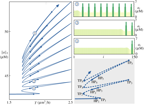
Fig. 3: Bifurcation diagram and selected solution patterns for the Smith model posed on a row of $150$ identical cells with Neumann boundary conditions at $i=1$ and free boundary conditions at $i=n$ (see Figure 2). Left: 2-norm of auxin concentration versus active transport parameter $T$. Right: as the snaking bifurcation diagram is ascended, new peaks are formed from the boundary towards the interior. Bottom-right: stable segments of the branch are found between Hopf bifurcations $\textrm{HP}_{2}$ and $\textrm{HP}_{3}$, $\textrm{HP}_{4}$ and $\textrm{HP}_{5}$, etc. Other secondary instabilities (not shown) are present along the unstable branches. Parameters: $D=1\,\mu\textrm{m}^{2}/\textrm{h}$, $\rho_{\textnormal{{\tiny IAA}}}=0.85\,\mu\textrm{M}/\textrm{h}$; other parameters as in Table 1.

In Figure 3 we show a branch of solutions of the Smith model for the 1D regular domain obtained with the parameter set in Table 1. We start the computation from the homogeneous solution at $T=0$ and follow the pattern for increasing values of $T$. As $T$ changes, we plot the $2$-norm of the auxin vector, $\|\bm{a}\|_{2}$, which is a measure of the spatial extent of the solution (the lower $\|\bm{a}\|_{2}$, the more localised the pattern) and denote stable (unstable) branches with solid (dashed) or thick (thin) lines.

The low peak found close to the boundary persists for increasing values of $T$ and grows steadily until we meet a first turning point (TP1). Before exploring the diagram in full, we compare our numerical findings with the analytical predictions of the asymptotic theory, valid for small $T$. The analytic asymptotic profile (10) gives a relative error $\|\bm{a}-(\bm{a}^{*}+T\bm{\alpha})\|_{2}/\|\bm{a}\|_{2}$ less than $0.4\%$ for $T\leq 0.2\;\mu\textrm{m}^{3}/\textrm{h}$, after which higher-order terms become predominant. This is shown in Figure 4 where we compare a branch of approximate solutions (magenta) to a branch of solutions to the full nonlinear problem (blue) for $D=1\,\mu\textrm{m}^{2}/\textrm{h}$ and small values of $T$.

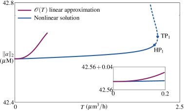
Fig. 4: Comparison between a branch of approximate linear $\mathcal{O}(T)$ solutions (magenta) and the corresponding branch of solutions to the full 2-component nonlinear system by Smith (blue) for a row of 150 identical cells with homogeneous Neumann boundary conditions at $i=0$ and free boundary conditions at $i=n$. The plot shows the 2-norm of the IAA concentration vector versus the continuation parameter $T$. Parameters as in Figure 3.

As we ascend the bifurcation diagram in Figure 3, new peaks are formed on the left side of the existing peaks, that is, towards the interior of the domain, until the whole domain is filled with peaks. We note that peaks are regularly spaced, as it was also observed in [5, 7, 57].

This bifurcation diagram resembles the one found for reaction–diffusion PDEs posed on the real line [40, 41, 42] except that here peaks are formed at the boundary rather than at the core of the domain. When peaks fill the entire domain, the branch enters an unstable irregular regime without snaking (not shown). Branches of solutions with peaks covering the entire domain are also present (not shown) and are partially discussed in Section 3.1.4.

Remark 3.1 (Biological interpretation of snaking).

The diagram in Figure 3 makes a plausible biological prediction for the formation of large peaks. A tissue composed of a string of cells, in the presence of passive diffusion, selects auxin patterns depending on the value of the active transport. Our analysis of the Smith model predicts that there exist two main regimes: for small $T$ there is a single low auxin peak at the boundary. As $T$ becomes larger, we enter a regime where the tissue can select from a large variety of auxin patterns. If, for instance $T\approx 1.9\mu\textrm{m}^{3}/h$, the tissue is able to select pattern 1, 2 or 3, which have a variable number of peaks. Therefore, the pattern selected in experiments depends highly upon the initial conditions of the system, similarly to what was reported by Jönsson and Krupinski [58]. As we shall see, a slanted version of the snaking bifurcation diagram is also present in 2D domains (both regular and irregular and for both the Smith and the Chitwood models).

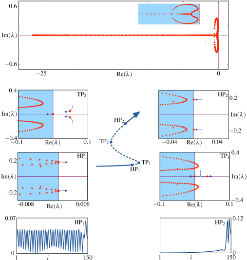
Fig. 5: Spectral computations of selected solution profiles. Top panel: spectrum of a stable solution point for $T<T_{\textrm{HP}_{1}}$. Middle panels: spectra at selected bifurcation points along the snaking bifurcation branch of Figure 3. Bottom panels: unstable eigenfunctions at $\textrm{HP}_{1}$ and $\textrm{HP}_{2}$. Parameters as in Figure 3.

3.1.3 Instabilities on the snaking branch

To understand if a solution pattern in stable to small perturbations we study in detail the eigenvalues of the Jacobian matrix (Result 4). The Jacobian matrix for the spatially-extended system (4)–(5) is sparse with a characteristic block structure determined by transport and diffusion terms (we refer the reader to [59] for a detailed description) and, for relatively small systems such as this one, eigenvalues are computed with dense linear algebra routines.

In this example, the solution with one small peak at the boundary becomes unstable at a Hopf bifurcation ($\textrm{HP}_{1}$) at $T\approx 2.1\;\mu\textrm{m}^{3}/\textrm{h}$, closely followed by other oscillatory instabilities and a saddle-node bifurcation ($\textrm{TP}_{1}$) at $T\approx 2.2\;\mu\textrm{m}^{3}/\textrm{h}$, after which the solution remains unstable. On the snaking branch, we find that saddle-node and Hopf bifurcations alternate regularly, as documented in Figure 3: saddle-node bifurcations align at $T\approx 1.9\;\mu\textrm{m}^{3}/\textrm{h}$ and $T\approx 2.5\;\mu\textrm{m}^{3}/\textrm{h}$, while Hopf bifurcations depart from each other as patterns become less localised. In this parameter setting, stable portions of the branch are delimited by two Hopf bifurcations, which, to the best of our knowledge, has not been reported before for snaking in reaction–diffusion systems. It should be noted, however, that Burke and Dawes [60] found Hopf bifurcations at the bottom of the snaking branch for an extended Swift–Hohenberg equation, which may lead to a bifurcation structure similar to the one in Figure 3 if secondary parameters are varied.

In Figure 5 we show spectra of solutions at selected points on the branch. Overall these spectra resemble those found in discretised advection-diffusion PDEs, with largely negative real eigenvalues associated with diffusion terms of the governing equations. In this context, however, increasing the number of cells does not alter the cell spacing, hence the spectrum does not grow in the negative real direction for larger system sizes.

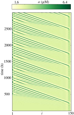
Fig. 6: Spatio-temporal state obtained via time simulation of the Smith model posed on a one-dimensional domain, close to the Hopf bifurcation $\textrm{HP}_{1}$. We set $T\gtrsim T_{HP_{1}}$ (and other parameters as in Figure 3) and use as initial condition a steady state with one peak at the boundary, obtained for $T\lesssim T_{HP_{1}}$. A long-time periodic auxin wave travels (and new auxin peaks are recruited) from the boundary towards the interior of the domain.

We monitored spectra of localised solutions as the snaking branch was ascended (see Figure 5): immediately after the Hopf bifurcation HP1, multiple eigenvalues cross the imaginary axis, therefore several oscillatory instabilities exist between $\textrm{HP}_{1}$ and $\textrm{TP}_{1}$ ($\textrm{HP}_{2}$ and $\textrm{TP}_{2}$, etc.). In the bottom panel of Figure 5 we show that the Hopf eigenfunction at $\textrm{HP}_{1}$ has a maximum near the boundary and the one for $\textrm{HP}_{2}$ is also spatially localised. We expect that branches of time-periodic (possibly spatially-localised) solutions emerge from the Hopf bifurcations. We have not observed stable small-amplitude oscillations in direct numerical simulations, but we report the existence of stable periodic states in which a temporal oscillation of the peak at $i=n$ initiates a wave of auxin moving towards the boundary at $i=1$, with long oscillation periods.

In Fig. 6 we show such a periodic solution obtained via time simulation in the neighbourhood of $\textrm{HP}_{1}$ (which is also visible in Figure 4). We set $T\gtrsim T_{\textrm{HP}_{1}}$ and use as initial condition a steady state (with one peak at the boundary), obtained for $T\lesssim T_{\textrm{HP}_{1}}$. In the resulting periodic state, auxin peaks are dynamically formed from the tip towards the interior of the domain: we point out that the period of oscillations (about 377 hours) is much greater than the period associated to the unstable Hopf eigenvalues. In addition, on such long time scales it is reasonable to assume that new cells are formed, so the geometry of the problem should change as well.

It was recently shown by Farcot and Yuan that, in one-dimensional flux-based models with no-flux boundary conditions, active transport is sufficient to elicit auxin oscillations [56]. In the concentration-based model considered here, oscillatory states in regular one-dimensional arrays are also found in a regime where active transport dominates over diffusion.

3.1.4 Changes in the auxin production parameter

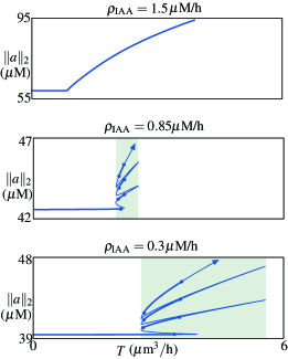
Fig. 7: Bifurcation diagrams of the Smith model for various values of the auxin production coefficient $\rho_{\textnormal{{\tiny IAA}}}$ (other parameters as in Figure 3). The lower the $\rho_{\textnormal{{\tiny IAA}}}$, the wider the snaking width and the stable branches. For sufficiently large values of $\rho_{\textnormal{{\tiny IAA}}}$ the snaking disappears and peaks form at once on a fully stable branch.

We conclude this primer on the 1D tissue by investigating the robustness of the snaking scenario described above (Results 5). In [59] it was shown that the auxin production parameter $\rho_{\textnormal{{\tiny IAA}}}$ has a significant influence on the solution profiles, therefore it is interesting to study how changes in this parameter affect the bifurcation structure. We repeated the numerical continuation of the Smith model for $20$ values of $\rho_{\textnormal{{\tiny IAA}}}$ in the interval $[0.3\;\mu\textrm{M}/\textrm{h},1.5\;\mu\textrm{M}/\textrm{h}]$. For low values of $\rho_{{}_{\textnormal{{\tiny IAA}}}}$, both the oscillatory instability $\textrm{HP}_{1}$ and the saddle node $\textrm{TP}_{1}$ move to the right and give rise to snaking bifurcation diagrams with increasingly wider stable segments (see Figure 7). As a consequence, in biological experiments where the auxin production was kept to a low value, the tissue would support multiple auxin patterns for a wider range of active transport coefficients. In the limit $\rho_{{}_{\textnormal{{\tiny IAA}}}}\ll\mu_{{}_{\textnormal{{\tiny IAA}}}}$ decay dominates over production, hence large peaks can not be sustained and indeed we find that the solution with a single small peak at the tip persists for very large values of $T$. This is in line with previous papers by Sahlin et al.[36] and De Reuille et al.[6] where it was postulated that auxin patterning demands a minimal level of auxin production within the tissue.

On the other hand, increasing $\rho_{\textnormal{{\tiny IAA}}}$ causes the snaking diagram to shrink and then disappear for $\rho_{\textnormal{{\tiny IAA}}}\geq 1.2\;\mu\textrm{M}/\textrm{h}$. In Figure 7 we show a fully stable branch for $\rho_{\textnormal{{\tiny IAA}}}=1.5\;\mu\textrm{M}/\textrm{h}$. On this branch peaks develop at once from the small-amplitude solution, without turning points. We mention however that for $\rho_{\textnormal{{\tiny IAA}}}$ between $1.2\;\mu\textrm{M}/\textrm{h}$ and $1.3\;\mu\textrm{M}/\textrm{h}$, Hopf bifurcations are found along the non-snaking branch (not shown), similar to what is found for the infinite domain [59].

As snaking branches distort, several types of secondary instabilities and collisions with neighbouring branches occur. In particular, we report codimension-2 Bogdanov–Takens bifurcations originating from the collision between $\textrm{TP}_{2}$ and $\textrm{HP}_{2}$, ($\textrm{TP}_{4}$ and $\textrm{HP}_{4}$, $\textrm{TP}_{6}$ and $\textrm{HP}_{6}$, etc.) when $\rho_{\textnormal{{\tiny IAA}}}$ is varied. The existence of these codimension-2 bifurcations could also be envisaged from the spectra in Figure 5. These instabilities, as the ones reported in the previous section, indicate that the tissue is capable of sustaining oscillations and dynamical auxin patterning, as well as steady states with multiple peaks. Dynamic states with spatio-temporal coherence (such as the one reported in Figure  6) are interesting from a biological standpoint [21], as they occur for the biologically plausible parameter values reported in Table 1. However, we could not find them in 2D domains with realistic parameter values, hence we do not discuss them further in this paper.

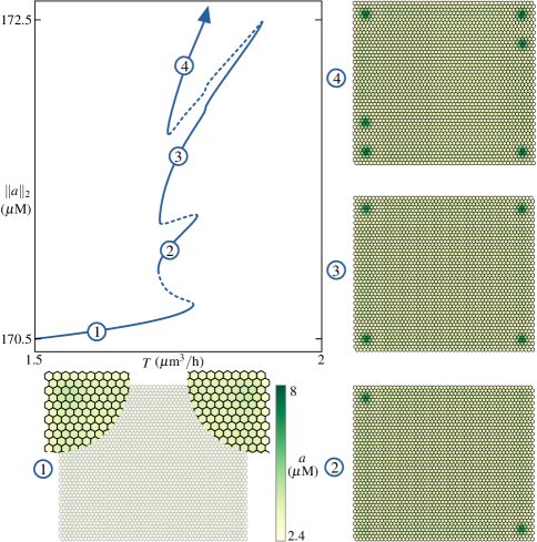
Fig. 8: Bifurcation diagram and selected solution patterns for the Smith model posed on a regular array of $50$ by $50$ hexagonal cells with 6 neighbours in the interior, 3 neighbours at the left and right edges and 4 neighbours at the top and bottom edges. Larger peaks are developed initially at the top-left and bottom-right corner (see also the values of the pre-factors $\xi_{i}$ in Figure 9) and new peaks are formed along the left and right edges, where we have fewer neighbours. Parameters: $D=1\,\mu\textrm{m}^{2}/\textrm{h}$, $\rho_{\textnormal{{\tiny IAA}}}=1.5\,\mu\textrm{M}/\textrm{h}$; other parameters as in Table 1.

3.2 Two-dimensional domains

We now move to more realistic geometries and study 2D domains with approximately square and circular boundaries, on which we prescribe free boundary conditions. In this Section we will revisit Results 1–6 in the 2D setting for both the Smith and the Chitwood models, so we refer the reader to the general summary in Section 2 and the 1D primer in Section 3.1.

The methods described in the previous section apply straightforwardly to the 2D case. In the first example we consider the Smith model on a grid of $50$ by $50$ hexagonal prismic cells with $l_{ij}=1\,\mu\textrm{m}$ and $V_{i}=3\sqrt{3}/2\,\mu\textrm{m}^{3}$. Cells have $6$ neighbours in the interior, $3$ neighbours at the left and right edges, and $4$ neighbours at the top and bottom edges. In this domain, corners are not all equal (see Figure 8) and we chose this configuration intentionally, to illustrate the influence of the number of neighbouring cells on the emerging patterns in 2D domains.

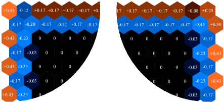
Fig. 9: Geometric pre-factors $\bm{\xi}$ at the top-left and top-right corners of the 2D regular domain of Figure 8. The interior set $\mathcal{I}$ is now clearly visible. Peaks and dips are proportional, for small $T$ and $D=0$, to the values of $\xi_{i}$. When $D\neq 0$ the largest peak is formed in the interior, close to the top/left corner and a smaller one is formed in the interior, towards the top/right corner.

Figure 9 shows the values of the geometric pre-factors $\bm{\xi}$ for 2 corners of the domain: our asymptotic analysis for $D=0\;\mu\textrm{m}^{2}/\textrm{h}$ (see the discussion in Section 3.1.1 and the generic derivation in Section 5) predicts the formation of peaks at the boundaries, with the highest peak at the top-left and bottom-right corners. Numerical computations for positive $D$ show that these peaks persist and become prominent for increasing $T$ (Figure 8, pattern 2). As in the one-dimensional case, patterns are arranged on a snaking bifurcation branch, even though in two-dimensions the snaking is slanted. Peaks arise initially in all four corners, then new spots are formed along the left and right edges (where cells have fewer neighbours), and then, for sufficiently large values of $\rho_{\textnormal{{\tiny IAA}}}$, along the top and bottom edges. In contrast with the 1D case, we have not found oscillatory bifurcations in this region of parameter space, so we conclude that stable portions of the branch are now delimited by turning points (see Figure 8). From a biological perspective, this means that patterns with peaks at the boundary are more likely to be observable in experiments, as they are stable in a wider region of parameter space.

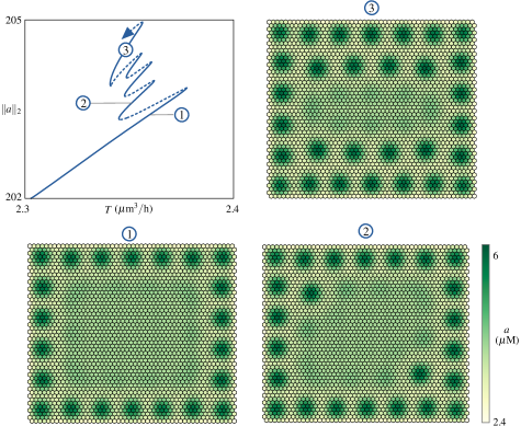
Fig. 10: Bifurcation diagram and selected solution patterns for the Chitwood model posed on the same domain of Figure 8 and a slightly larger value of the auxin production coefficient ($\rho_{{}_{\textnormal{{\tiny IAA}}}}=2\mu\textrm{M}/\textrm{h}$, $D=1\,\mu\textrm{m}^{2}/\textrm{h}$ and other parameters are as in Table 1). A ring of peaks is developed at the boundary, owing to the increased value of $\rho_{\textnormal{{\tiny IAA}}}$. Other spots are formed in pairs (pattern 2), until they fill a full row (pattern 3) and the whole domain (not shown).

In a second example, we consider the Chitwood model posed on the 2D regular domain, using the parameters of Table 1. Remarkably, the resulting bifurcation diagram (not shown) is analogous to the one found in Figure 8 for the Smith model. As a further confirmation, we tested the robustness of the snaking mechanism to changes in the auxin production coefficient, as it was done for the 1D case in Figure 7. We set $\rho_{\textnormal{{\tiny IAA}}}=2\,\mu\textrm{M}/\textrm{h}$ and show in Figure 10 the corresponding bifurcation diagram and solution patterns. While active transport remains responsible for the selection of peaks towards the boundary, the interplay with auxin production allows the formation of a ring of spots at the boundary as opposed to single spots at the corners (see pattern 1 in Figure 10). After the first turning point, spots are formed in pairs (pattern 2), until they fill a full row (pattern 3) and the whole domain (not shown). As in Section 3.1.4, the auxin production coefficient has a large influence on the resulting peaks. For this 2D regular domain, we also scanned several values of the auxin production coefficient and confirmed that comparatively high values of $\rho_{\textnormal{{\tiny IAA}}}$ induce the formation of peaks all-at-once (similar to top panel of Figure 7), hence a fully patterned tissue is possible without a Turing bifurcation.

Fig. 11: Bifurcation diagram and selected solution patterns for the Smith model for an almost-circular domain of $742$ irregular cells (geometry taken from [55]). We find an irregular and slanted bifurcation diagram with stable portion delimited by saddle-node bifurcations. Parameters: $D=1\,\mu\textrm{m}^{2}/\textrm{h}$, $\rho_{\textnormal{{\tiny IAA}}}=1.5\,\mu\textrm{M}/\textrm{h}$; other parameters as in Table 1.

Fig. 12: Bifurcation diagram and selected solution patterns for the Chitwood model for an almost-circular domain of $742$ irregular cells (geometry taken from [55]). We find an irregular and slanted bifurcation diagram with stable portion delimited by saddle-node bifurcations. Parameters: $D=1\,\mu\textrm{m}^{2}/\textrm{h}$, $\rho_{\textnormal{{\tiny IAA}}}=1.5\,\mu\textrm{M}/\textrm{h}$; other parameters as in Table 1.

In the remaining 2 examples, $742$ irregular prismic cells cover an almost-circular domain in a realistic tissue with free boundary conditions (see Figure 11, whose geometry has been extracted from [55]). Even though the asymptotic analysis is not valid for irregular arrays, we expect results to be qualitatively similar if cellular volumes and contact areas do not vary greatly from cell to cell. In these examples the number of neighbours varies over the domain; however, the cells at the boundaries have predominantly fewer neighbours and this is where peaks are formed initially. The bifurcation diagram is now plotted in terms of the scaled bifurcation parameter $T/\langle l_{ij}\rangle$, where $\langle\cdot\rangle$ denotes the average in the tissue (so far we have considered cases where $\langle l_{ij}\rangle=1\,\mu\textrm{m}$, so the following diagrams are directly comparable with the ones above). We note that in this domain $\langle l_{ij}\rangle\approx 13.26\,\mu\textrm{m}$ and $\langle V_{i}\rangle\approx 294\,\mu\textrm{m}^{3}$. As in the 2D regular cases, stable portions of the branch are enclosed between consecutive saddle-nodes bifurcations and there are no oscillatory instabilities on the stable branches. Figure 11 shows the results for the Smith model: as usual, peaks are formed initially at the boundary and then fill the interior (see pattern 4), and the slanted snaking ensures the existence of stable solutions with localised peaks in a wide regime of the parameter $T$.

When we pose Chitwood model on the same irregular domain, the results are strikingly similar, as seen in Figure 12: peaks form initially at the top-left quadrant of the circular domain (see patterns 1 and 2 in Figures 11 and 12), confirming that it is the geometry of the tissue to drive the spots location. An inspection of the fully patterned tissues (patterns 4 in Figures 11 and 12) reveal that model parameters and functional forms for the active transport functions have an influence on the size and structure of the peaks. Variations in $\rho_{{}_{\textnormal{{\tiny IAA}}}}$ also confirmed the trend seen in Figure 7 (not shown).

4 Discussion

In this paper we investigated the origin of auxin peaks in generic concentration-based models and proposed a robust mechanism for their formation over short time scales, using a combination of asymptotic and numerical bifurcation analysis.

The asymptotic calculations, valid for a class of models with identical cells and weak active transport, show that peaks emerge as boundary corrections to the homogeneous steady state: the peak amplitude depends on the local geometry and is higher in regions where cells have fewer neighbours, that is, next to the boundary. Crucially, this is a direct consequence of the mathematical structure of the models considered here (Hypotheses 1–2): since the active transport depends on the number of neighbours at distance $2$ from the $i$th cell via the geometric coefficients $\xi_{i}$, then deviations from the homogeneous state will always appear at the boundaries, where the number of neighbours is different from the interior of the tissue. This mechanism is different from (and not in contrast with) the Turing bifurcation scenario reported in previous studies on unbounded domains: on finite tissues, peaks do not emerge from instabilities of the flat state, but they simply morph from it for low values of $T$. The most immediate consequence of our mathematical analysis is that, in concentration-based models, active transport and geometry concur to promote localisation of auxin peaks [11].

In irregular domains, a similar asymptotic analysis can be carried out, but the peak selection mechanism in this case also depends on the cellular volumes and contact areas, so we can not exclude a priori that peaks will form in the interior as well as on the boundary. A statistical characterisation of the peaks location in relation to the variance of the cellular array is possible and should be considered in future studies.

The two models by Smith [5] and Chitwood [34] fit in the framework discussed above and, for these systems, we have provided numerical evidence that peaks persist for moderate and large values of the active transport rate $T$: large-amplitude peaks are arranged on a snaking branch, which becomes slanted in 2D tissues. A major implication of the numerical findings of Figures 11–12 is that localised auxin peaks are observable: a slow experimental sweep in the active transport from low to high values should reveal an initial localisation of the peaks, which then progressively de-localise and fill the domain. Conversely, if the active transport is kept constant, the tissue should be able to select from more than one pattern, depending on the initial condition.

Since snaking is now recognised as the footprint of localisation in a wide variety of nonlinear media, we expect that bifurcation diagrams similar to the ones shown in this paper for the Smith and the Chitwood models might also arise generically. One class of models that are of interest and can be analysed via numerical bifurcation analysis are flux-based auxin models, which have not been studied in this paper. While numerical continuation is readily applicable to such models, they are likely to require a separate analytic treatment, as some of them do not possess the factorisation presented in Hypothesis 2.

Importantly, we find that the bifurcation scenario is influenced by the auxin production rate, since the selectable configurations depend sensitively on the balance between auxin production and active transport. The results in Figure 7 (also confirmed by the 2D irregular calculations of Figures 11 and 12) support the conclusion that if auxin production rate was decreased quasi-statically, either actively or passively, the organism would be able to switch from fully-patterned states to configurations with few peaks at the boundary. In addition, since the parameters of the concentration-based models considered here are scaled by cellular volumes, we expect tissues with different cell sizes to behave similarly: in tissues with larger $V$, the snaking limits are expected to occur for larger values of $T$, so as to keep the ratio $T/V$ constant (and a similar reasoning is valid for the passive transport parameter $D$).

The conclusion reported above are naturally limited to experiments that are well approximated by concentration-based models, and for the plausible biological parameter values selected in the original papers by Smith et al. [5] and Chitwood et al. [34]. We note that an experimental validation of the predictions presented here requires the ability to detect changes in the auxin distribution during development. An experimental technique that could help testing the predictions of these two models is the one recently proposed by Brunoud et al. [53], which allows to visualise auxin with high spatio-temporal resolution. We note that it would be possible to apply numerical bifurcation analysis also to a modified model that accounted for markers’ dynamics and auxin-sensor interactions.

A further desirable property of the experimental setup would be the ability to stimulate auxin peaks locally (thereby changing initial conditions) and test whether the tissue settles to a new equilibrium. In view of the large uncertainty on the parameter values of the models, we expect our predictions to agree qualitatively with experimental results.

5 Materials and Methods

In this section we present an analytical framework to construct steady state solutions featuring localised auxin peaks in generic concentration-based models.

5.1 Asymptotic derivation of peak solutions

We begin by giving a generic definition of concentration-based models in the absence of diffusion: as mentioned above, several examples from literature can be cast in this form.

Definition 5.1 (Concentration-based model without diffusion).

A concentration-based model without diffusion is a set of $m\times n$ ODEs of the form

$$\dot{\bm{y}}_{i}=\bm{\pi}(\bm{y}_{i})-\bm{\delta}(\bm{y}_{i})+T\sum_{j\in\mathcal{N}_{i}}\bm{\nu}_{ji}(\bm{y}_{1},\ldots,\bm{y}_{n})-\bm{\nu}_{ij}(\bm{y}_{1},\ldots,\bm{y}_{n}),\qquad i=1,\ldots,n,$$ (11)

where $\bm{\pi},\bm{\delta}\colon\mathbb{R}_{+}^{m}\to\mathbb{R}_{+}^{m}$, are the production and decay functions, respectively, $T\in\mathbb{R}_{+}$, is the (nonnegative) active transport parameter, $\{1,\ldots,n\}$ are vertices of a static undirected graph $G$, $\mathcal{N}_{i}\subseteq\{1,2,\ldots,n\}$ is the set of neighbours of cell $i$, containing $|\mathcal{N}_{i}|$ elements and $\bm{\nu}_{ij}:\mathbb{R}_{+}^{m}\times\cdots\times\mathbb{R}_{+}^{m}\to\mathbb{R}_{+}^{m}$ are the active transport functions. We will assume $\bm{\pi}$, $\bm{\delta}$ and $\bm{\nu}_{ij}$ to be smooth vector fields depending on a set of control parameters $\bm{p}\in\mathbb{R}^{p}_{+}$, but we omit this dependence for simplicity and write, for instance, $\bm{\pi}(\bm{y}_{i})$ instead of $\bm{\pi}(\bm{y}_{i};\bm{p})$.

Remark 5.1.

Concrete examples of concentration based models in this form can be found in section 5.1.1 an section 5.1.2

We now prove the following result

Lemma 5.1.

Let us consider the concentration-based model (11) and let us suppose that there exist vector-valued functions $\bm{\psi}\colon\mathbb{R}_{+}^{m}\times\mathbb{R}_{+}^{m}\to\mathbb{R}_{+}^{m}$ and $\bm{\varphi}\colon\mathbb{R}_{+}^{m}\to\mathbb{R}_{+}^{m}$ such that

$$\bm{\nu}_{ij}(\bm{y}_{1},\ldots,\bm{y}_{n})=\bm{\psi}(\bm{y}_{i},\bm{y}_{j})\odot\bm{\varphi}(\bm{y}_{j})\oslash\sum_{k\in\mathcal{N}_{i}}\bm{\varphi}(\bm{y}_{k}),\qquad\text{for all $i,j=1,\ldots,n$,}$$ (12)

where $\odot$ and $\oslash$ denote the standard Hadamard product and division between vectors. Further, let $\bm{y}^{*}\in\mathbb{R}^{m}$ be such that $\bm{\pi}(\bm{y}^{*})=\bm{\delta}(\bm{y}^{*})$, $\bm{\psi}(\bm{y}^{*},\bm{y}^{*})\neq\mathbf{0}$ and $\bm{\varphi}(\bm{y}^{*})\neq 0$, then

1. If $T=0$ or all cells have the same number of neighbours, $|\mathcal{N}_{i}|=|\mathcal{N}^{*}|$, then the homogeneous solution $(\bm{y}^{*},\ldots,\bm{y}^{*})^{\textnormal{T}}\in\mathbb{R}^{nm}$ is a steady state for the concentration-based model.

2. If $0<T\ll 1$ and cells have different number of neighbours and the Jacobian matrix $\bm{\pi}^{\prime}(\bm{y}^{*})-\bm{\delta}^{\prime}(\bm{y}^{*})$ is nonsingular, then a inhomogeneous steady state (to leading order) is given by

   $$\bm{y}_{i}=\bm{y}^{*}+\xi_{i}T\big{[}\bm{\pi}^{\prime}(\bm{y}^{*})-\bm{\delta}^{\prime}(\bm{y}^{*})\big{]}^{-1}\bm{\psi}(\bm{y}^{*},\bm{y}^{*}),\qquad i=1,\ldots,n$$

   where the coefficients $\xi_{i}$ depend on the local properties of the cellular array, namely

   $$\xi_{i}=1-\sum_{j\in\mathcal{N}_{i}}\frac{1}{|\mathcal{N}_{j}|}.$$

Proof.

If $T=0$ the statement is clearly true, so henceforth we assume $T\neq 0$. Since $\bm{\pi}(\bm{y}^{*})-\bm{\delta}(\bm{y}^{*})=\mathbf{0}$, the right-hand side of (11) vanishes for all $i$ if $|\mathcal{N}_{i}|=|\mathcal{N}_{j}|=|\mathcal{N}^{*}|$. On the other hand, if not all cells have the same number of neighbours and $T$ is small, we may seek for asymptotic steady states in the form $\bm{y}_{i}=\bm{y}^{*}+T\bm{\eta}_{i}+\mathcal{O}(T^{2})$ for $i=1,\dots,n$ and $(\bm{\eta}_{i})_{j}=\mathcal{O}(1)$. A Taylor expansion of the right-hand side around $(\bm{y}^{*},\ldots,\bm{y}^{*})^{\textnormal{T}}\in\mathbb{R}^{nm}$ gives, to leading order,

$$\mathbf{0}=\bm{\pi}(\bm{y}^{*})-\bm{\delta}(\bm{y}^{*})+T[\bm{\pi}^{\prime}(\bm{y}^{*})-\bm{\delta}^{\prime}(\bm{y}^{*})]\bm{\eta}_{i}+T\sum_{j\in\mathcal{N}_{i}}\bm{\nu}_{ji}(\bm{y}^{*},\ldots,\bm{y}^{*})-\bm{\nu}_{ij}(\bm{y}^{*},\ldots,\bm{y}^{*}),$$ (13)

In order to find an expression for $\bm{\eta}_{i}$, we evaluate the sums in (13):

$$\begin{split}\sum_{j\in\mathcal{N}_{i}}&\bm{\nu}_{ji}(\bm{y}^{*},\ldots,\bm{y}^{*})-\bm{\nu}_{ij}(\bm{y}^{*},\ldots,\bm{y}^{*})\\ &=\sum_{j\in\mathcal{N}_{i}}\bigg{(}\bm{\psi}(\bm{y}^{*},\bm{y}^{*})\odot\bm{\varphi}(\bm{y}^{*})\oslash\sum_{k\in\mathcal{N}_{j}}\bm{\varphi}(\bm{y}^{*})-\bm{\psi}(\bm{y}^{*},\bm{y}^{*})\odot\bm{\varphi}(\bm{y}^{*})\oslash\sum_{k\in\mathcal{N}_{i}}\bm{\varphi}(\bm{y}^{*})\bigg{)}\\ &=\bm{\psi}(\bm{y}^{*},\bm{y}^{*})\sum_{j\in\mathcal{N}_{i}}\bigg{(}\frac{1}{|\mathcal{N}_{j}|}-\frac{1}{|\mathcal{N}_{i}|}\bigg{)},\\ &=-\xi_{i}\bm{\psi}(\bm{y}^{*},\bm{y}^{*})\end{split}$$ (14)

and combining (13) with (14) we obtain the assert. ∎

Remark 5.2 (Small-amplitude peak solutions).

In finite regular arrays, cells in the interior have all the same number of neighbours, so we can use these properties to give formal definitions of interior and boundary sets

$$\mathcal{I} =\left\{i\in\left\{1,\ldots,n\right\}\left|1-\sum_{j\in\mathcal{N}_{i}}\frac{1}{|\mathcal{N}_{j}|}=0\right.\right\},$$

$$\mathcal{B} =\left\{1,\ldots,n\right\}\setminus\mathcal{I}.$$

In passing, we note that $\mathcal{B}$ contains in general more cells than the physical boundary. Lemma 5.1 shows that, to leading order, steady states for small $T$ deviate from the homogeneous solutions only in $\mathcal{B}$, where auxin peaks and dips are proportional to $T$ and $\xi_{i}$, namely

$$\bm{y}_{i}=\begin{cases}\bm{y}^{*}&\text{if $i\in\mathcal{I}$,}\\ \bm{y}^{*}+\xi_{i}T\big{[}\bm{\pi}^{\prime}(\bm{y}^{*})-\bm{\delta}^{\prime}(\bm{y}^{*})\big{]}^{-1}\bm{\psi}(\bm{y}^{*},\bm{y}^{*})&\text{if $i\in\mathcal{B}$.}\\ \end{cases}$$ (15)

Remark 5.3 (Irregular domains).

Lemma 2.1 can not be applied in general if the domain is irregular, that is, if cells have different volumes and contact lengths: if, say, the active transport function $\bm{\nu}_{ij}$ depends explicitly on the cellular volume $V_{i}$ and the $V_{i}$ are not all equal, then it is not possible to express $\bm{\nu}_{ij}$ as in (12). However the theory can be extended to the case of irregular domains. We do not report this derivation here, but note that it features, as expected, cellular volumes and contact areas.

5.1.1 One-dimensional domain and one component per cell

As an example, we consider the Smith model [5] with constant fixed PIN1 amount, posed on a one-dimensional array of identical cells with volume $V$, Neumann boundary conditions at $i=1$ and free boundary conditions at $i=n$. The Neumann boundary conditions are obtained by considering ghost cells [59], therefore boundary and interior sets are given by $\mathcal{I}={1,\ldots,n-2}$ and $\mathcal{B}=\{n-1,n\}$, respectively. Furthermore we denote by $p$ the fixed PIN concentration and apply Lemma 5.1 with $m=1$, $y_{i}=a_{i}$ and

$$\pi\colon a\mapsto\frac{\rho_{{}_{\textnormal{{\tiny IAA}}}}}{1+\kappa_{{}_{\textnormal{{\tiny IAA}}}}a}, \delta\colon a\mapsto-\mu_{\textnormal{{\tiny IAA}}}a,$$

$$\psi\colon(a,b)\mapsto\frac{p}{V}\frac{a^{2}}{1+\kappa_{T}b^{2}}, \varphi\colon a\mapsto\exp(c_{1}a),$$

where all parameters are assumed to be strictly positive. By balancing production and decay terms we find the positive homogeneous state

$$a^{*}=\frac{-1+\sqrt{1+4\kappa_{\textnormal{{\tiny IAA}}}\rho_{\textnormal{{\tiny IAA}}}/\mu_{\textnormal{{\tiny IAA}}}}}{2\kappa_{\textnormal{{\tiny IAA}}}}.$$

In the absence of active transport, $a^{*}$ is a stable steady state of the model since $\pi^{\prime}(a^{*})-\delta^{\prime}(a^{*})<0$. For $0\neq T\ll 1\,\mu\textrm{m}^{3}/\textrm{h}$, $\bm{a}^{*}$ is not a steady state since $\mathcal{B}$ is nonempty and $\xi_{n-1}=-1/2$, $\xi_{n}=1/2$, hence we obtain, to leading order

$$a_{i}=\begin{cases}a^{*}&\text{for $i=1\ldots n-2$,}\\[10.00002pt] a^{*}+T\dfrac{p}{2V}\bigg{[}\dfrac{\rho_{\textnormal{{\tiny IAA}}}\kappa_{\textnormal{{\tiny IAA}}}}{1+\kappa_{\textnormal{{\tiny IAA}}}(a^{*})^{2}}+\mu_{\textnormal{{\tiny IAA}}}\bigg{]}^{-1}\dfrac{(a^{*})^{2}}{1+\kappa_{T}(a^{*})^{2}}&\text{for $i=n-1$,}\\[10.00002pt] a^{*}-T\dfrac{p}{2V}\bigg{[}\dfrac{\rho_{\textnormal{{\tiny IAA}}}\kappa_{\textnormal{{\tiny IAA}}}}{1+\kappa_{\textnormal{{\tiny IAA}}}(a^{*})^{2}}+\mu_{\textnormal{{\tiny IAA}}}\bigg{]}^{-1}\dfrac{(a^{*})^{2}}{1+\kappa_{T}(a^{*})^{2}}&\text{for $i=n$.}\end{cases}$$

5.1.2 One-dimensional domain and two components per cell

The Smith model [5] features 2 ODEs per cell. If we pose this model on a one-dimensional array of identical cells, the graph $G$ associated to the nodes is the same as in our previous example, hence $\mathcal{B}$, $\mathcal{I}$ and $\bm{\xi}$ are unchanged. We can now apply Lemma 5.1 with $m=2$, $\bm{y}_{i}=(a_{i},p_{i})^{\textrm{T}}$ and

$$\bm{\pi}\colon\begin{bmatrix}a\\ p\end{bmatrix}\mapsto\begin{bmatrix}\dfrac{\rho_{\textnormal{{\tiny IAA}}}}{1+\kappa_{\textnormal{{\tiny IAA}}}a}\\[10.00002pt] \dfrac{\rho_{\textnormal{{\tiny PIN}}_{0}}+\rho_{\textnormal{{\tiny PIN}}}a}{1+\kappa_{\textnormal{{\tiny PIN}}}p}\\ \end{bmatrix}, \bm{\delta}\colon\begin{bmatrix}a\\ p\end{bmatrix}\mapsto\begin{bmatrix}-\mu_{\textnormal{{\tiny IAA}}}a\\ -\mu_{\textnormal{{\tiny PIN}}}p\\ \end{bmatrix},$$

$$\bm{\psi}\colon\bigg{(}\begin{bmatrix}a\\ p\end{bmatrix},\begin{bmatrix}b\\ q\end{bmatrix}\bigg{)}\mapsto\begin{bmatrix}\dfrac{p}{V}\dfrac{a^{2}}{1+\kappa_{T}b^{2}}\\[10.00002pt] 0\end{bmatrix}, \bm{\varphi}\colon\begin{bmatrix}a\\ p\end{bmatrix}\mapsto\begin{bmatrix}\exp(c_{1}a)\\ 0\end{bmatrix}.$$

Balancing production and decay terms we find a homogeneous strictly positive steady state for $T=0$

$$\bm{y}^{*}=\begin{bmatrix}a^{*}\\ b^{*}\end{bmatrix}=\begin{bmatrix}\dfrac{-1+\sqrt{1+4\kappa_{\textnormal{{\tiny IAA}}}\rho_{\textnormal{{\tiny IAA}}}/\mu_{\textnormal{{\tiny IAA}}}}}{2\kappa_{\textnormal{{\tiny IAA}}}}\\[10.00002pt] \dfrac{-1+\sqrt{1+4\kappa_{\textnormal{{\tiny PIN}}}(\rho_{\textnormal{{\tiny PIN}}_{0}}+\rho_{\textnormal{{\tiny PIN}}}a^{*})/\mu_{\textnormal{{\tiny PIN}}}}}{2\kappa_{\textnormal{{\tiny PIN}}}}\\ \end{bmatrix}$$

which is stable since

$$\operatorname{Spec}(\bm{\pi}^{\prime}(\bm{y}^{*})-\bm{\delta}^{\prime}(\bm{y}^{*}))=\left\{-\frac{\rho_{\textnormal{{\tiny IAA}}}\kappa_{\textnormal{{\tiny IAA}}}}{(1+\kappa_{\textnormal{{\tiny IAA}}}a^{*})^{2}}-\mu_{\textnormal{{\tiny IAA}}},\;-\frac{(\rho_{\textnormal{{\tiny PIN}}_{0}}+\rho_{\textnormal{{\tiny PIN}}}a^{*})\kappa_{\textnormal{{\tiny PIN}}}}{(1+\kappa_{\textnormal{{\tiny PIN}}}a^{*})^{2}}-\mu_{\textnormal{{\tiny PIN}}}\right\}$$

Since the parameters are assumed to be positive with the exception of $\rho_{\textnormal{{\tiny PIN}}_{0}}$ which is nonnegative (see also Table  1 ) we do not have a zero eigenvalue.

The inverse of $\bm{\pi}^{\prime}(\bm{y}^{*})-\bm{\delta}^{\prime}(\bm{y}^{*})$ can be computed explicitly and for $T\ll 1\,\mu\textrm{m}^{3}/\textrm{h}$ we obtain to leading order

$$a_{i}=\begin{cases}a^{*}&\text{for $i=1\ldots n-2$,}\\[10.00002pt] a^{*}+T\dfrac{p}{2V}\bigg{[}\dfrac{\rho_{\textnormal{{\tiny IAA}}}\kappa_{\textnormal{{\tiny IAA}}}}{1+\kappa_{\textnormal{{\tiny IAA}}}(a^{*})^{2}}+\mu_{\textnormal{{\tiny IAA}}}\bigg{]}^{-1}\dfrac{(a^{*})^{2}}{1+\kappa_{T}(a^{*})^{2}}&\text{for $i=n-1$,}\\[10.00002pt] a^{*}-T\dfrac{p}{2V}\bigg{[}\dfrac{\rho_{\textnormal{{\tiny IAA}}}\kappa_{\textnormal{{\tiny IAA}}}}{1+\kappa_{\textnormal{{\tiny IAA}}}(a^{*})^{2}}+\mu_{\textnormal{{\tiny IAA}}}\bigg{]}^{-1}\dfrac{(a^{*})^{2}}{1+\kappa_{T}(a^{*})^{2}}&\text{for $i=n$,}\end{cases}$$

$$p_{i}=\begin{cases}p^{*}&\text{for $i=1\ldots n-2$,}\\[25.00003pt] p^{*}+T\dfrac{p}{2V}\dfrac{\bigg{[}\dfrac{\rho_{\textnormal{{\tiny PIN}}}}{1+\kappa_{\textnormal{{\tiny PIN}}}p^{*}}\bigg{]}\bigg{[}\dfrac{(a^{*})^{2}}{1+\kappa_{T}(a^{*})^{2}}\bigg{]}}{\bigg{[}\dfrac{\rho_{\textnormal{{\tiny IAA}}}\kappa_{\textnormal{{\tiny IAA}}}}{(1+\kappa_{\textnormal{{\tiny IAA}}}a^{*})^{2}}+\mu_{\textnormal{{\tiny IAA}}}\bigg{]}\bigg{[}\dfrac{(\rho_{\textnormal{{\tiny PIN}}_{0}}+\rho_{\textnormal{{\tiny PIN}}}a^{*})\kappa_{\textnormal{{\tiny PIN}}}}{(1+\kappa_{\textnormal{{\tiny PIN}}}p^{*})^{2}}+\mu_{\textnormal{{\tiny PIN}}}\bigg{]}}&\text{for $i=n-1$,}\\[25.00003pt] p^{*}-T\dfrac{p}{2V}\dfrac{\bigg{[}\dfrac{\rho_{\textnormal{{\tiny PIN}}}}{1+\kappa_{\textnormal{{\tiny PIN}}}p^{*}}\bigg{]}\bigg{[}\dfrac{(a^{*})^{2}}{1+\kappa_{T}(a^{*})^{2}}\bigg{]}}{\bigg{[}\dfrac{\rho_{\textnormal{{\tiny IAA}}}\kappa_{\textnormal{{\tiny IAA}}}}{(1+\kappa_{\textnormal{{\tiny IAA}}}a^{*})^{2}}+\mu_{\textnormal{{\tiny IAA}}}\bigg{]}\bigg{[}\dfrac{(\rho_{\textnormal{{\tiny PIN}}_{0}}+\rho_{\textnormal{{\tiny PIN}}}a^{*})\kappa_{\textnormal{{\tiny PIN}}}}{(1+\kappa_{\textnormal{{\tiny PIN}}}p^{*})^{2}}+\mu_{\textnormal{{\tiny PIN}}}\bigg{]}}&\text{for $i=n$.}\end{cases}$$

Another example of a concentration based transport model that features 2 ODEs per cell is the Chitwood model [34]. The model is given by

$$\bm{\pi}\colon\begin{bmatrix}a\\ p\end{bmatrix}\mapsto\begin{bmatrix}\dfrac{\rho_{\textnormal{{\tiny IAA}}}}{1+\kappa_{\textnormal{{\tiny IAA}}}a}\\[10.00002pt] \dfrac{\rho_{\textnormal{{\tiny PIN}}_{0}}+\rho_{\textnormal{{\tiny PIN}}}a}{1+\kappa_{\textnormal{{\tiny PIN}}}p}\\ \end{bmatrix}, \bm{\delta}\colon\begin{bmatrix}a\\ p\end{bmatrix}\mapsto\begin{bmatrix}-\mu_{\textnormal{{\tiny IAA}}}a\\ -\mu_{\textnormal{{\tiny PIN}}}p\\ \end{bmatrix},$$

$$\bm{\psi}\colon\bigg{(}\begin{bmatrix}a\\ p\end{bmatrix},\begin{bmatrix}b\\ q\end{bmatrix}\bigg{)}\mapsto\begin{bmatrix}\dfrac{p}{V}\dfrac{\exp{c_{2}\ a}-1}{\exp{c_{2}\ b}}\\[10.00002pt] 0\end{bmatrix}, \bm{\varphi}\colon\begin{bmatrix}a\\ p\end{bmatrix}\mapsto\begin{bmatrix}\exp(c_{1}a)\\ 0\end{bmatrix}.$$

For the same domain as above and with $m=2$ and $\bm{y}_{i}=(a_{i},p_{i})^{\textrm{T}}$ we can apply Lemma 5.1.

The homogeneous steady state for $T=0$ is the same as for the Smith model and for $T\ll 1\,\mu\textrm{m}^{3}/\textrm{h}$ we obtain to leading order

$$a_{i}=\begin{cases}a^{*}&\text{for $i=1\ldots n-2$,}\\[10.00002pt] a^{*}+T\dfrac{p}{2V}\bigg{[}\dfrac{\rho_{\textnormal{{\tiny IAA}}}\kappa_{\textnormal{{\tiny IAA}}}}{1+\kappa_{\textnormal{{\tiny IAA}}}(a^{*})^{2}}+\mu_{\textnormal{{\tiny IAA}}}\bigg{]}^{-1}\dfrac{\exp{(c_{2}\ a^{*})}-1}{\exp{(c_{2}\ a^{*})}}&\text{for $i=n-1$,}\\[10.00002pt] a^{*}-T\dfrac{p}{2V}\bigg{[}\dfrac{\rho_{\textnormal{{\tiny IAA}}}\kappa_{\textnormal{{\tiny IAA}}}}{1+\kappa_{\textnormal{{\tiny IAA}}}(a^{*})^{2}}+\mu_{\textnormal{{\tiny IAA}}}\bigg{]}^{-1}\dfrac{\exp{(c_{2}\ a^{*})}-1}{\exp{(c_{2}\ a^{*})}}&\text{for $i=n$,}\end{cases}$$

$$p_{i}=\begin{cases}p^{*}&\text{for $i=1\ldots n-2$,}\\[25.00003pt] p^{*}+T\dfrac{p}{2V}\dfrac{\bigg{[}\dfrac{\rho_{\textnormal{{\tiny PIN}}}}{1+\kappa_{\textnormal{{\tiny PIN}}}p^{*}}\bigg{]}\bigg{[}\dfrac{(a^{*})^{2}}{1+\kappa_{T}(a^{*})^{2}}\bigg{]}}{\bigg{[}\dfrac{\rho_{\textnormal{{\tiny IAA}}}\kappa_{\textnormal{{\tiny IAA}}}}{(1+\kappa_{\textnormal{{\tiny IAA}}}a^{*})^{2}}+\mu_{\textnormal{{\tiny IAA}}}\bigg{]}\bigg{[}\dfrac{(\rho_{\textnormal{{\tiny PIN}}_{0}}+\rho_{\textnormal{{\tiny PIN}}}a^{*})\kappa_{\textnormal{{\tiny PIN}}}}{(1+\kappa_{\textnormal{{\tiny PIN}}}p^{*})^{2}}+\mu_{\textnormal{{\tiny PIN}}}\bigg{]}}&\text{for $i=n-1$,}\\[25.00003pt] p^{*}-T\dfrac{p}{2V}\dfrac{\bigg{[}\dfrac{\rho_{\textnormal{{\tiny PIN}}}}{1+\kappa_{\textnormal{{\tiny PIN}}}p^{*}}\bigg{]}\bigg{[}\dfrac{(a^{*})^{2}}{1+\kappa_{T}(a^{*})^{2}}\bigg{]}}{\bigg{[}\dfrac{\rho_{\textnormal{{\tiny IAA}}}\kappa_{\textnormal{{\tiny IAA}}}}{(1+\kappa_{\textnormal{{\tiny IAA}}}a^{*})^{2}}+\mu_{\textnormal{{\tiny IAA}}}\bigg{]}\bigg{[}\dfrac{(\rho_{\textnormal{{\tiny PIN}}_{0}}+\rho_{\textnormal{{\tiny PIN}}}a^{*})\kappa_{\textnormal{{\tiny PIN}}}}{(1+\kappa_{\textnormal{{\tiny PIN}}}p^{*})^{2}}+\mu_{\textnormal{{\tiny PIN}}}\bigg{]}}&\text{for $i=n$.}\end{cases}$$

5.1.3 Two-dimensional domain of identical hexagonal cells

Lemma 5.1 also applies when the Smith or the Chitwood model are posed on a two-dimensional array of identical hexagonal cells. In this case, the computations for $\bm{y}^{*}$ are identical to the previous example and the asymptotic derivation is also straightforward. Instead of writing the full expressions for $\mathcal{B}$, $\mathcal{I}$ and $\bm{\xi}$, we refer the reader to Figure 9, where the values of $\bm{\xi}$ are shown for two corners of the domain. As claimed in Section 7, the highest peaks occur at the top-left and right-bottom corners.

5.2 Models with diffusion

We can extend the definition of concentration-based models to the case where diffusion is present.

Definition 5.2 (Concentration-based model with diffusion).

A concentration-based model with diffusion is a set of $mn$ ODEs of the form

$$\dot{\bm{y}}_{i}=\bm{\pi}(\bm{y}_{i})-\bm{\delta}(\bm{y}_{i})+\bm{D}\sum_{j\in\mathcal{N}_{i}}(\bm{y}_{j}-\bm{y}_{i})+T\sum_{j\in\mathcal{N}_{i}}\bm{\nu}_{ji}(\bm{y}_{1},\ldots,\bm{y}_{n})-\bm{\nu}_{ij}(\bm{y}_{1},\ldots,\bm{y}_{n}),$$ (16)

for $i=1,\ldots,n$, where $\bm{D}\in\mathbb{R}^{m\times m}$ is a diagonal diffusion matrix and all other quantities are as in Definition 5.1

Remark 5.4.

Reasoning like in Lemma 5.1, we obtain $\bm{y}_{i}=\bm{y}^{*}+T\bm{\eta}_{i}+\mathcal{O}(T^{2})$ where $\bm{\eta}_{i}$ satisfy

$$\left[\bm{J(\bm{y}^{*})}+\bm{L}\otimes\bm{D}\right]\begin{bmatrix}\bm{\eta}_{1}\\ \vdots\\ \bm{\eta}_{n}\end{bmatrix}=\begin{bmatrix}\xi_{1}\bm{\psi}(\bm{y}^{*},\bm{y}^{*})\\ \vdots\\ \xi_{n}\bm{\psi}(\bm{y}^{*},\bm{y}^{*})\end{bmatrix},$$

$\bm{J}(\bm{y})\in\mathbb{R}^{mn\times mn}$ is block-diagonal with blocks $\bm{\pi}^{\prime}(\bm{y}^{*})-\bm{\delta}^{\prime}(\bm{y}^{*})$, $\bm{L}\in\mathbb{R}^{n\times n}$ is the Laplacian matrix associated to the graph $G$ with Neumann boundary conditions and $\otimes$ denotes the Kronecker product between matrices. The operator $\bm{L}\otimes\bm{D}$ is negative semi-definite and it has a zero eigenvalue, corresponding to a constant eigenvector. However, summing this matrix to $\bm{J}(\bm{y})=\bm{\pi}^{\prime}(\bm{y}^{*})-\bm{\delta}^{\prime}(\bm{y}^{*})$, makes the resulting linear operator non-singular.

In the presence of diffusion we can not directly apply the formula (15), even for regular cellular arrays: owing to diffusion, cells in $\mathcal{I}$ will also deviate from the homogeneous state, hence peaks and dips are not necessarily formed within $\mathcal{B}$, but may occur in interior cells that are close to the boundary. First-order corrections for these cases can be computed analytically using Chebyshev polynomials [61] or numerically using linear algebra routines. Even though we report below an example of this calculation, we point out that in practice this is not necessary, since the numerical bifurcation software gives access to the full nonlinear solution and to its linear stability.

5.2.1 One-dimensional domain with diffusion and two components per cell

We return to the Smith model with $m=2$, posed on a row of identical cells, and we now add diffusion only in the auxin component.

The expressions for $a^{*}$ and $p^{*}$ are unchanged from Section 5.1.2, as is the first order approximation of $p_{i}$ (since there is no diffusion for $p$). Expressions for the first-order approximations in $a_{i}$ are more involved: proceeding as explained above for generic models with diffusion, we obtain, to leading order

$$\left[\left(\dfrac{\rho_{{}_{\textnormal{{\tiny IAA}}}}\kappa_{{}_{\textnormal{{\tiny IAA}}}}}{\left(1+\kappa_{{}_{\textnormal{{\tiny IAA}}}}a^{*}\right)^{2}}+\mu_{{}_{\textnormal{{\tiny IAA}}}}\right)\left(\begin{array}[]{ccccc}1&0&\ldots&\ldots&0\\ 0&1&0&\ldots&0\\ &&\ddots&&\\ &&&\ddots&\\ 0&\ldots&\ldots&0&1\end{array}\right)+\dfrac{D}{V}\left(\begin{array}[]{ccccc}-1&1&&&\\ 1&-2&1&&\\ &\ddots&\ddots&\ddots&\\ &&1&-2&1\\ &&&1&-1\end{array}\right)\right]$$ (27)

$$\cdot\left(\begin{array}[]{c}\eta_{1}\\ \eta_{2}\\ \vdots\\ \vdots\\ \eta_{n}\end{array}\right)=\left(\begin{array}[]{c}\xi_{1}\psi\left(\bm{a}^{*},\bm{p}^{*}\right)\\ \xi_{2}\psi_{2}\left(\bm{a}^{*},\bm{p}^{*}\right)\\ \vdots\\ \vdots\\ \xi_{n}\psi_{n}\left(\bm{a}^{*},\bm{p}^{*}\right)\end{array}\right)=\left(\begin{array}[]{c}0\\ \vdots\\ 0\\ \frac{1}{2}\psi_{n-1}\left(\bm{a}^{*},\bm{p}^{*}\right)\\ -\frac{1}{2}\psi_{n}\left(\bm{a}^{*},\bm{p}^{*}\right)\end{array}\right).$$ (43)

Solving this linear equation above led to the approximate solution profiles in Figure 2 and the red solution branch in Figure 4. The same derivation and figures can be obtained for the Chitwood model (not shown).

References

- [1] Scarpella E, Marcos D, Friml J, Berleth T. Control of leaf vascular patterning by polar auxin transport. Genes & Development. 2006;20:1015–1027.
- [2] Band L, Wells D, Larrieu A, Sun J, Middleton A, French A, et al. Root gravitropism is regulated by a transient lateral auxin gradient controlled by a tipping-point mechanism. PNAS. 2012;109(12):4668–4673.
- [3] Lavenus J, Goh T, Roberts I, Guyomarch́ S, Lucas M, De Smet I, et al. Lateral root development in Arabidopsis: fifty shades of auxin. Trends in Plant Science. 2013;18(8):450–458.
- [4] de Wit M, Lorrain S, Fankhauser C. Auxin-mediated plant architectural changes in response to shade and high temperature. Physiol Plant. 2014;151(1):13-24.
- [5] Smith RS, Guyomarc’h S, Mandel T, Reinhardt D, Kuhlemeier C, Prusinkiewicz P. A plausible model of phyllotaxis. PNAS. 2006;103(5):1301–1306.
- [6] De Reuille P, Bohn-Courseau I, Ljung K, Morin H, Carraro N, Godin C, et al. Computer simulations reveal properties of the cell–cell signaling network at the shoot apex in Arabidopsis. PNAS. 2006;103(5):1627–1632.
- [7] Jönsson H, Heisler M, Shapiro B, Meyerowitz E, Mjolsness E. An auxin-driven polarized transport model for phyllotaxis. PNAS. 2006;103(5):1633–1638.
- [8] Kuhlemeier C. Phyllotaxis. Trends Plant Sci. 2007;12(4):143–150.
- [9] Jonsson H, Gruel J, Krupinski P, Troein C. On evaluating models in Computational Morphodynamics Current Opinion in Plant Biology. 2012;15:103-110.
- [10] Benková E, Michniewicz M, Sauer M, Teichmann T, Seifertová D, Jürgens G, et al. Local, efflux-dependent auxin gradients as a common module for plant organ formation. Cell. 2003;115:591–602.
- [11] Heisler M, Ohno C, Das P, Sieber P, Reddy G, Long J, et al. Patterns of Auxin Transport and Gene Expression during Primordium Development Revealed by Live Imaging of the Arabidopsis Inflorescence Meristem. Current Biology. 2005;15:1899–1911.
- [12] Grieneisen V, Xu J, Maree A, Hogeweg P, Scheres B. Auxin transport is sufficient to generate a maximum and gradient guiding root growth. Nature. 2007;449:1008–1013.
- [13] Jones AR, Kramer E, Knox K, Swarup R, Bennett MJ, Lazarus CM, et al.. Auxin transport through non-hair cells sustains root hair development. Nat. Cell Biol. 2008;11:78-84.
- [14] Brena-Medina V, Champneys AR, Grierson C, Ward MJ. Mathematical Modelling of Plant Root Hair Initiation: Dynamics of Localized Patches. SIAM J Appl Dyn Syst. 2013;13(1):210–248.
- [15] Berleth T, Scarpella E, Prusinkiewicz P. Towards the systems biology of auxin-transport-mediated patterning. Trends in Plant Science. 2007;12:151-159.
- [16] Stoma S, Lucas M, Chopard J, Schaedel M, Traas J, Godin C. Flux-Based Transport Enhancement as a Plausible Unifying Mechanism for Auxin Transport in Meristem Development. PLoS Comput Biol. 2008;4(10):e1000207.
- [17] Kramer E, Bennett M. Auxin transport: a field in flux. Trends in Plant Science. 2006;11:382–386.
- [18] Wabnik K, Govaerts W, Friml J, Kleine-Vehn J. Feedback models for polarized auxin transport: an emerging trend. Molecular bioSystems. 2011;7:2352–2359.
- [19] Swarup R, Kramer E, Perry P, Knox K, Leyser H, Haseloff J, et al. Root gravitropism requires lateral root cap and epidermal cells for transport and response to a mobile auxin signal. Nature Cell Biology. 2005;7:1057–1065.
- [20] Wabnik K, Kleine-Vehn J, Balla J, Sauer M, Naramoto S, Reinohl V, et al. Emergence of tissue polarization from synergy of intracellular and extracellular auxin signalling. Mol Syst Biol. 2010;6:447.
- [21] Merks R, Van de Peer Y, Inz D, Beemster G. Canalization without flux sensors: a traveling-wave hypothesis. Trends Plant Sci. 2007;12(9):384–390.
- [22] Mitchison G. The polar transport of auxin and vein patterns in plants. Phil Trans R Soc Lond B. 1981;295:461–471.
- [23] van Berkel K, de Boer R J, Scheres B, ten Tusscher K. Polar auxin transport: models and mechanisms. Development, 2013;140(11):2253-2268.
- [24] Krupinski P, Jönsson H. Modeling auxin-regulated development. Cold Spring Harb Perspect Biol. 2010;2(2):001560.
- [25] Kramer E. Computer models of auxin transport: a review and commentary. Journal of Experimental Botany. 2008;59:45–53.
- [26] Rolland-Lagan A, Prusinkiewicz P. Reviewing models of auxin canalization in the context of leaf vein pattern formation in arabidopsis. Plant J. 2005;44(5)854–865.
- [27] Band L, Fozard J, Godin C, Jensen O, Pridmore T, MJ B, et al. Multiscale Systems Analysis of Root Growth and Development: Modeling Beyond the Network and Cellular Scales. The Plant Cell Online. 2012;24(10):3892–3906.
- [28] Feugier F, Mochizuki A, Iwasa Y. Self-organization of the vascular system in plant leaves: inter-dependent dynamics of auxin flux and carrier proteins. Journal of Theoretical Biology. 2005;236:366–375.
- [29] Kramer E, Rutshow H, Mabie S. AuxV: a database of auxin transport velocities. Trends in Plant Science. 2011;16:461–463.
- [30] Steinacher A, Leyser O, Clayton R. A computational model of auxin and pH dynamics in a single plant cell. Journal of Theoretical Biology. 2012;296:84–94.
- [31] Heisler M, Jönsson H. Modeling auxin transport and plant development. Journal of Plant Growth Regulation. 2006;25:302–312.
- [32] Bilsborough G, Runions A, Markoulas M, Jenkins H, Hasson A, Galinha C, et al. Model for the regulation of arabidopsis thaliana leaf margin development. Proceedings of the National Academy of Sciences. 2011;108:3424–3429.
- [33] Krauskopf B, Osinga H, Galán-Vioque J. Numerical Continuation methods for Dynamical Systems. Springer. 2007.
- [34] Chitwood DH, Headland LR, Ranjan A, Martinez CC, Braybrook SA, Koenig DP, Kuhlemeier C, Smith RS, Sinhaa NR. Leaf Asymmetry as a Developmental Constraint Imposed by Auxin-Dependent Phyllotactic Patterning. The Plant Cell. 2012;24:1–10.
- [35] Bayer EM, Smith RS, Mandel T, Nakayama N, Sauer M, Prusinkiewicz P, Kuhlemeier C. Integration of transport-based models for phyllotaxis and midvein formation. Genes Development. 2009;23:373–384.
- [36] Sahlin P, Söderberg B, Jönsson H. Regulated transport as a mechanism for pattern generation: Capabilities for phyllotaxis and beyond. Journal of Theoretical Biology. 2009;258:60-70.
- [37] Newell AC, Shipman PD, Sun Z. Phyllotaxis: Cooperation and competition between mechanical and biochemical processes. Journal of Theoretical Biology. 2008;251:421–439.
- [38] Knobloch E. Spatially localized structures in dissipative systems: open problems. Nonlinearity. 2008;21(4):45–60.
- [39] Woods P, Champneys A. Heteroclinic tangles and homoclinic snaking in the unfolding of a degenerate reversible hamiltonian-hopf bifurcation. Physica D: Nonlinear Phenomena. 1999;129(3-4):147–170.
- [40] Burke J, Knobloch E. Homoclinic snaking: structure and stability. Chaos. 2007;17(3):037102.
- [41] Burke J, Knobloch E. Snakes and ladders: localized states in the swift-hohenberg equation. Physics Letters A. 2007;360(6):681–688.
- [42] Beck M, Knobloch J, Lloyd D, Sandstede B, Wagenknecht T. Snakes, ladders, and isolas of localised patterns. SIAM J Math Anal. 2009;41(3):936–972.
- [43] Chapman S, Kozyreff G. Exponential asymptotics of localized patterns and snaking bifurcation diagrams. Physica D. 2009;238:319–354.
- [44] Lloyd D, Sandstede B, Avitabile D, Champneys A. Localized hexagon patterns of the planar Swift-Hohenberg equation. SIAM J Appl Dynam Syst. 2008;7:1049–1100.
- [45] Avitabile D, Lloyd D, Burke J, Knobloch E, Sandstede B. To snake or not to snake in the planar swift-hohenberg equation. SIAM J Appl Dyn Syst. 2010;9:704–733.
- [46] Beaume C, Bergeon A, Knobloch E. Convectons and secondary snaking in three-dimensional natural doubly diffusive convection. Physics of fluids. 2013;25(2):024105.
- [47] Jacono D, Bergeon A, Knobloch E, et al. Three-dimensional spatially localized binary-fluid convection in a porous medium. Journal of Fluid Mechanics. 2013;730:R2.
- [48] Taylor C, Dawes J. Snaking and isolas of localised states in bistable discrete lattices. Physics Letters A. 2010;375(1):14–22.
- [49] Coombes S, Lord G, Owen M. Waves and bumps in neuronal networks with axo-dendritic synaptic interactions. Physica D: Nonlinear Phenomena. 2003;178(3-4):219–241.
- [50] Laing C, Troy W. PDE methods for nonlocal models. SIAM Journal on Applied Dynamical Systems. 2003;2(3):487–516.
- [51] Rankin J, Avitabile D, Baladron J, Faye G, D L. Continuation of localised coherent structures in nonlocal neural field equations. SIAM Journal of Scientific Computation. 2014;36(1):B70–B93.
- [52] Avitabile D, Schmidt H. Snakes and ladders in an Inhomogeneous neural field model. Physica D. 2015;294: 24–-36
- [53] Brunoud G, Wells D, Oliva M, Larrieu A, Mirabet V, Burrow A, et al. A novel sensor to map auxin response and distribution at high spatio-temporal resolution. Nature. 2012;482:103–106.
- [54] Beemster G, Baskin T. Analysis of cell division and elongation underlying the developmental acceleration of root growth in Arabidopsis thaliana. Plant Physiology. 1998;116:515–526.
- [55] Merks R, Guravage M, Inzé D, Beemster G. VirtualLeaf: An Open-Source Framework for Cell-Based Modeling of Plant Tissue Growth and Development. Plant Physiology. 2011;155(2):656-666.
- [56] Farcot E, Yuan Y. Homogeneous Auxin Steady States and Spontaneous Oscillations in Flux-Based Auxin Transport Models. SIAM Journal of Applied Dynamical Systems. 2013;12(3):1330–1353.
- [57] Reinhardt D, Pesce E, Stieger P, Mandel T, Baltensperger K, Bennett M, Traas J, Friml JC, Kuhlemeier C. Regulation of phyllotaxis by polar auxin transport. Nature. 2003;426:255-260.
- [58] Jonsson H, Krupinski P. Modeling plant growth and pattern formation. Current Opinion in Plant Biology. 2010;13:5–11.
- [59] Draelants D, Broeckhove J, Beemster T, W V. Numerical bifurcation analysis of the pattern formation in a cell based auxin transport model. Journal of Mathematical Biology. 2013;67(5):1279–1305.
- [60] Burke J, Dawes J. Localized states in an extended swift-Hohenberg equation. SIAM Journal on Applied Dynamical Systems. 2012;11(1):261–284.
- [61] Arfken G, Brown G, Weber HJ, Ruby L. Mathematical methods for physicists. Academic Press. 1985;.