Memory endowed US cities and their demographic interactions

Abstract

A quantitative understanding of cities’ demographic dynamics is becoming a potentially useful tool for planning sustainable growth. The concomitant theory should reveal details of the cities’ past and also of its interaction with nearby urban conglomerates for providing a reasonably complete picture. Using the exhaustive database of the Census Bureau in a time window of 170 years, we exhibit here empirical evidence for time and space correlations in the demographic dynamics of US counties, with a characteristic memory-time of 25 years and typical distances of interaction of 200 km. These correlations are much larger than those observed in an European country (Spain), giving to the US a more coherent evolution. We also measure the resilience of US cities to historical events, finding a demographical post-traumatic amnesia after wars (as the Civil War) or economic crisis (as the 1929 Stock Market Crash).

I Introduction

A half of the human population lives in urban areas pop . Asking whether the present population’s growth rates are economically and ecologically sustainable is a recurrent question pop2 that justifies efforts directed towards the development of quantitative unified theories of urban living betwest . A countless number of degrees of freedom is involved in a city’s evolution, host of individual contributions, involving millions of people, acting on their own free will. Devising a unified theory constitutes a formidable challenge. However, despite this intrinsic difficulty, many advances have been made in the last years. During the XX century many regularities were reported, such as Zipf’s Law in the city-population rank distribution zipf ; mbat2 ; power ; X1 ; nosPLA09 , or the celebrated Gibrat’s Law of proportional growth applicable to cities gibrat0 ; gibrat ; city1 ; city2 ; nosJRSI13 ; nosJRSI14 . In addition, empirical data show that the scaling with population of internal degrees of freedom in an urban body such as i) the structure of road networks or urban sprawl patterns gibrat ; diff ; roads2 ; and ii) metrics such as wages or crime rates lbet2 ; PnasW , both follow predictable tendencies that can be mathematically described. In addition to a city’s growth, electoral processes and many other social phenomena have been successfully modelled as well santo ; firms ; 1sta ; oppi ; power ; nosPLA09 ; nosEPJB10 . Also, collective modes emerge when cities are considered as entities that evolve and interact in a coherent fashion. The interaction between cities nosJRSI14 (as measured by, for instance, by the number of crossed phone calls gmodel or human mobility mob1 ) displays predictable characteristics. Indeed, an analogy between the evolution of the population of an ensemble of cities and the random movement of particles in a fluid was made by conjoining Gibrat’s Law of proportional growth with Brownian motion. In such an approach the size $X$ at time $t$ of the $i$-th geometrical Brownian walker follows the dynamical equationgibrat0 ; city1 ; city2 ; gibrat ; nosEPJB12b ; nosJRSI13

$$\dot{X}_{i}(t)=X_{i}(t)v_{i}(t),$$ (1)

where the dot denotes a time-derivative and $v_{i}(t)$ is the growth rate, which is described as a Wiener coefficient with covariance $\mathrm{Cov}[v_{i}(t),v_{j}(t^{\prime})]=\sigma_{v}^{2}\delta_{ij}\delta(t-t^{\prime})$ —$\delta$ standing for the delta function and $\sigma_{v}$ for the standard deviation of the growth rates— i.e., uncorrelated and memoryless dynamics. Considering a new variable defined as $u_{i}(t)=\ln X_{i}(t)$ nosEPJB12b , we recover all the properties of the physical Ideal Gas in what one may call the scale-free ideal gas nosPA10 ; nosJRSI13 . Exhaustive empirical observations of the dynamics of Spain’s population demonstrates that this analogy can be used to formulate a Thermodynamics of population flows nosPRE12 . Moreover, we have recently shown that this assumption of uncorrelated evolution fails for cities that are close neighbors nosJRSI14 . Additionally, the evolution of cities-population exhibits memory, indicating that we deal with a non-Markovian process. These results are indicative of i) a rich and complex phenomenology underlying population flows, and ii) that our models should go beyond the Ideal Gas to include pairwise interactions and inertia, as in the case of real gases in Statistical Physics. The presence of some kind of correlations has been also independently proposed in Ref. mbat2 , where it is shown via numerical experiments that it is necessary to introduce conditioned sampling to reproduce Zipf’s Law, simulating what the authors call ‘coherence’. These advances, both in the internal structure and the functionality of cities, as well as in the properties of an ensemble of interacting cities, encourage the searching for a unified theory.

II Results

II.1 Stochastic properties of US growth rates

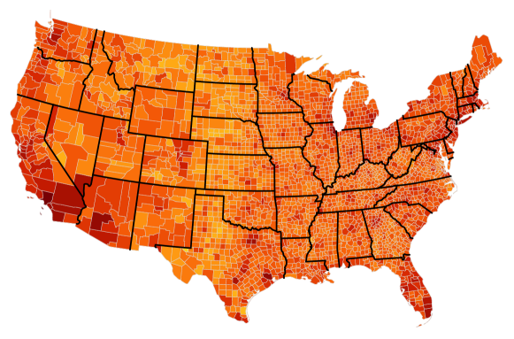
We look for quantitative space-time patterns underlying US demographics and ascertain which trends are universal and which are local by comparison with Ref. nosJRSI14 for Spanish cities. An exhaustive analysis of the US population is made using the Census Boreau database of counties’ population census . We have used data from 1830 to 2000 (170 years), in a time window that covers relevant historical events such as the Civil War, both World Wars, and the 1929 Stock Market Crash. More than 3000 counties (all of them with available data) are considered in our study, whose spatial distribution is depicted in Fig. 1. We verified the validity of Gibrat’s Law, including the correction for smaller populations, discovered in Ref. nosJRSI13 . To this effect we added a new term to the proportional law, a ’finite size noise’ (FSN) of the form

$$\dot{X}_{i}(t)=X_{i}(t)v_{i}(t)+\sqrt{X_{i}(t)}w_{i}(t),$$ (2)

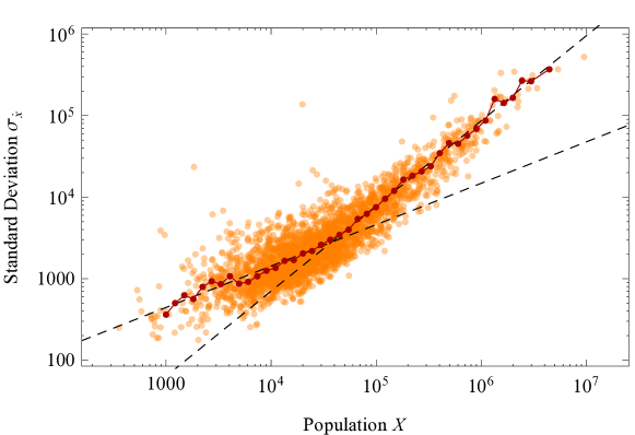
where $w_{i}(t)$ is an independent Wiener coefficient. This term is a direct consequence of the Central Limit Theorem, as shown in Refs. nosJRSI13 ; nosPRE12 , due to the independent nature of the $w_{i}(t)$. The variation of the population $X_{i}$ is much smaller than the variation of the growth rates. Thus, for the later, the standard deviation $\sigma_{\dot{x}}$ in our time windows becomes

$$\sigma_{\dot{x}}(X_{i})\cong X_{i}\sigma_{v}+\sqrt{X_{i}}\sigma_{w},$$ (3)

where $\sigma_{v}$ and $\sigma_{w}$ are the deviations of the proportional and finite size noise, respectively. Results are displayed in Fig. 1. It is clear that the median of the deviations, as a function of the county population, follows 1) a FSN trend for $X<35000$ inhabitants, and 2) proportional growth for $X>35000$. Remarkably enough, a linear fit to the log-log representation —where power laws become straight lines with slope-values linked to the exponents— gives for the exponents $0.508\pm 0.025$ (with $\log(\sigma_{w})=2.6\pm 0.2$) for the first trend and $1.04\pm 0.02$ (with $\log(\sigma_{v})=-3.1\pm 0.2$) for the second one, with a coefficient of determination $R^{2}$ of $0.96$ and $0.994$, respectively. Since these values almost coincide with the expected ones ($1/2$ and $1$), we can regard the Gibrat plus FSN Law as verified, a rather significant observation.

II.2 Measuring memory

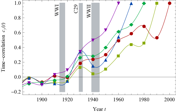
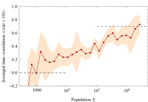
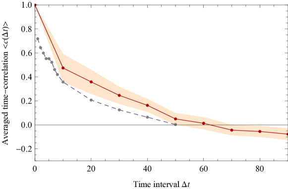
To check whether US counties exhibit memory effects, we appeal to the Pearson’s product-moment correlation coefficient $c_{y}(t)=\mathrm{Corr}[\dot{X}(y),\dot{X}(t)]$, using as samples the list of counties’ growth rates for i) the year $y$ and ii) any precedent time $t$ for which data are available. We find that the averaged time-correlation over $n_{y}=12$ samples (from 1890 to 2000), defined as $\langle c(\Delta t)\rangle=n_{y}^{-1}\sum_{y}c_{y}(y+\Delta t)$ and calculated for consecutive census instantiations ($\Delta t=10$ years), shows a behavior similar to that found for Spanish cities nosJRSI14 : large cities exhibit greater inertia. We can attribute the smaller counties’ loss of memory to the FSN term, which becomes important for them (see Fig. 2a). For larger intervals of time $\Delta t$, we find a clear decay of the averaged time-correlation. Remarkably enough, the correlations are much larger than those found for Spanish cities (Fig. 2b). Considering only the first 50 years, a fit to an exponential decay gives us a characteristic time of $25\pm 7$ years ($R^{2}=0.990$), but surprisingly enough, the correlation eventually becomes negative after $\sim 60$ years.

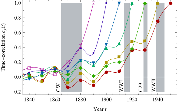
In order to gain a deeper understanding of this unexpected trend, and also to check whether it is caused by a non-homogeneous behavior of the correlations, we have independently studied all the contributions $c_{y}(t)$ for several years $y$ (and precedent times $t$). We find that, although for all $y$ a decay of the correlation with time is always present, historical events clearly modulate these correlations. For the growth rates from 1890 to 1950, we find that, irrespective of the year, no memory remains in the demographics of US counties from the years that precede the Civil War, in a kind of ‘post-traumatic amnesia’. For the second half of the XX century, we find, in general, a slower decay —larger memory— than for other time-periods. The most important historical event that one immediately detects (by simple inspection) regarding the cities’ memory is the economic crisis after the 1929 Stock Market Crash. Again, irrespective of the year, one still encounters (i) a correlation’s fall and (ii) loss of memory regarding precedent decades. Thus, instead of an homogeneous year-independent decay of the correlations with time, we find a decay with a strong dependence on historical events. However, some unanswered questions remain —as 1) why do the years 1940 and 1950 seem to be not much afflicted by amnesia? or 2) the reason for the strong fluctuations between the years 1990 and 2000. Accordingly, more research along this line of ‘quantitative History’ remains to be undertaken.

II.3 Measuring interactions

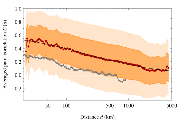
We consider now spatial correlations. The pairwise Pearson product-moment correlation coefficient $C_{ij}=\mathrm{Corr}[\dot{X}_{i},\dot{X}_{j}]$ of the $i$ and $j$-th counties is obtained using as samples the evolution of the growth rates of each county in a given time window. We speak here of the XX century, from 1900 to 2000 (10 sample sets). We compare the value obtained per each pair with the distance between counties $d_{ij}$. The averaged value —obtained as $C(d)=\sum_{ij}C_{ij}\delta(d-d_{ij})/\sum_{ij}\delta(d-d_{ij})$— exhibits a clear dependence on distance, demonstrating the entanglement between US populations-nuclei. The tail of the decay displays a long-range behavior (see Fig. 4), and the pertinent curve can be nicely fitted to an analytical expression of the form

$$C(d)=\frac{C(0)}{1+|d/d_{0}|^{\alpha}},$$ (4)

with $C(0)=0.62\pm 0.02$, $d_{0}=215\pm 32$ km, and $\alpha=0.71\pm 0.04$, for a $R^{2}$ coefficient of $0.997$. Remarkably, the correlations are much larger that those observed for Spain nosJRSI14 , with a larger characteristic distance (215 US vs. 80 km for Spanish cities) and a much slower decay ($\alpha=0.71$). Note that for an inverse-square law, $\alpha=2$.

The comparison between USA and Spain is illustrated by Fig. 4. Results confirm the conjecture that US cities evolve in a more coherent fashion that the cities in Spain, notwithstanding the fact that the US surface is 20 times larger than Spain’s, while its population is 6.5 times larger. We may speak of an integration-coherence for US cities that seems to be lacking in Europe, as has also been proposed in Ref. mbat2 : Zipf’s Law emerges when the largest US cities are considered but not when this is done on a state-by-state basis, whereas in Europe, Zipf’s law emerges for each country as a whole, and not when all the European continent is considered. The standard deviation observed for the US is of $\sim 0.4$ and does not change with distance. The expected theoretical width for a bivariate normal distribution for the same number of samples is $1/3$ biv , a 20% smaller than the measured one. Thus, we gather that additional factors are involved in the US pairwise correlation. One can attribute to the distance-factor an 80% of the city-city entanglement. We expect that some of these extra contributions could be associated to local factors, such as the transportation network, the particular socio-economical status of the city, and/or special historical links between some population-nuclei. A detailed analysis of the pairwise correlations of a selected county –instead of the coarse-grained viewpoint adopted here— when crossed with other relevant metrics, may help to gain a deeper understanding of the particular demographic and/or economic status, present and future, of a given urban area.

III Summary and conclusions

Demographic US patterns display a rich and complex phenomenology, including both space and time correlations. US cities exhibit a strong link with their past. In an exercise of quantitative History, we have found that relevant historical events, such as the Civil War and the 1929 economic crisis, leave a strong imprint in the demographic dynamics, that one may call a ‘post-traumatic amnesia’. The spatial correlations, much larger than those observed in Europe, indicate a high level of coherence and suggest that the evolution of any single city can not be understood without taking the whole collective of cities into account. We feel that these empirical findings are relevant to understanding the country at a collective macroscopic level. Also, some microscopic insights are gained that may help city planners to improve their panoply of tools census ; tools2 .

A)

B)

Figure 1: A) spatial distribution map and population of US counties census (the darker, the larger population). B) Standard deviation $\sigma$ of county’s growth rate as a function of the total population $X$ (orange dots). The median (red line and dots) clearly follows the proportional Gibrat’s law for populations larger than $35000$ inhabitants (slope 1 in a log-log representation), while it follows the expected trend of finite size noise for smaller populations (slope 1/2). Dashed lines follow the linear fit performed per each contribution (see text).

A)

B)

Figure 2: Averaged time-correlations in population growth. A) Averaged time-correlations after 10 years $\langle c(\Delta t=10)\rangle$ versus town-sizes $X$ (dot-line). The shaded area represents the width determined by one standard deviation. Horizontal dashed lines are asymptotic levels to follow the decrease of the correlation at lower populations. B) Averaged time-correlation $\langle c(\Delta t)\rangle$ for the relative growth of towns populated by more that 10,000 inhabitants. Shaded areas represent widths determined by one standard deviation. The time-correlation for Spanish cities is also shown for comparison’s sake (grey line and dots).

A)

B)

Figure 3: Time-correlations in population growth $c_{y}(t)$ of the year $y$ with all previous years denoted by $t$. Historical events as the Civil War (CW), the First World War (WWI), the 1929 Stock Market Crash (C29), and the Second World War (WWII), are marked with shadows. A) Correlations for years $y=1950$ (red circles), 1940 (yellow squares), 1930 (green diamonds), 1920 (turquoise up-triangles), 1910 (blue down-triangles), 1900 (navy small circles), and 1890 (purple empty squares). In all cases, the correlation becomes almost zero after the Civil War. B) Correlations for the last half of XX century: years $y=2000$ (red circles), 1990 (yellow squares), 1980 (green diamonds), 1970 (blue up-triangles), and 1960 (purple down-triangles). A general pattern of decay is apparent for all years, and remarkably, the five curves drop after the Stock Market Crash of 1929.

Figure 4: Pairwise correlation $C$ versus distance between counties $d$. The mean value for a given distance is indicated (red line and dots) together with one standard deviation (darker shadow) and by two of them (lighter shadow). The black line follows the analytical fit of Eq. (4). The spatial correlation for Spanish cities is also shown for comparison’s sake (grey line and dots).

References

- (1) UN-Habitat, State of the World’s Cities 1010/2011 — Cities for All: Bridging the Urban Divide (2010) www.unhabitat.org
- (2) Schellnhuber HJ, Molina M, Stern N, Huber V, Kadner S. Global Sustainability: A Nobel Cause (Cambridge Univ. Press, 2010)
- (3) Bettencourt L, West G. A unified theory of urban living Nature 467, 912 (2010)
- (4) Cristelli M, Batty M, Pietronero L. There is more than a Power Law in Zipf Scientific Reports 2, 812 (2012)
- (5) Zipf GK. Human Behavior and the Principle of Least Effort (Addison-Wesley, Cambridge, MA, 1949).
- (6) Newman MEJ. Power laws, Pareto distributions and Zipf’s law. Contemp Phys 46, 323 (2005)
- (7) Baek SK, Bernhardsson S, Minnhagen P Zipf’s law unzipped, New J Phys 13, 043004 (2011) .
- (8) Hernando A, Puigdomènech D, Villuendas D, Vesperinas C, Plastino A. Zipf’s law from a Fisher variational-principle, Phys Lett A 374, 18 (2009)
- (9) Gibrat R Les Inégalités économiques, (Librairie du Recueil, Sirey, Paris, 1931).
- (10) Rozenfeld H, Rybski D, Andrade JS, Batty M, Stanley HE, Makse HA (2008) Laws of Population Growth, Proc Natl Acad Sci USA 105:18702.
- (11) Gabaix X, Ioannides YM. Handbook of Regional and Urban Economics, Vol. 4 (North-Holland, Amsterdam, 2004).
- (12) Blank A, Solomon S. Power laws in cities population, financial markets and internet sites (scaling in systems with a variable number of components), Physica A 287, 279 (2000)
- (13) Hernando A, Hernando R, Plastino A,Plastino AR. The workings of the maximum entropy principle in collective human behaviour, J R Soc Interface 10, 20120758 (2013)
- (14) Hernando A, Hernando R, Plastino A. Space-time correlations in urban sprawl, J R Soc Interface 11, 20130930 (2013)
- (15) Makse HA, Andrade JS, Batty M, Havlin S, Stanley HE. Modelling urban growth patterns with correlated percolation, Phys. Rev. E, 58, 7054 (1998)
- (16) Masucci AP, Stalinov K, Batty M. Limited Urban Growth: London’s Street Network Dynamics since the 18th Century, PLoS One, 8, e69469 (2013)
- (17) L. Bettencourt. Science 340, 1438 (2013).
- (18) Bettencourt LMA, Lobo J, Helbing D, Kuehnert C, West GB. Growth,. Innovation, Scaling, and the Pace of Life in Cities, Proc Natl Acad Sci USA 104, 7301 (2007)
- (19) Chatterjee A, Mitrovič M, Fortunato S. Scientific Reports 3, 1049 (2013)
- (20) Axtell RL. Zipf Distribution of U.S. Firm Sizes, Science 293, 1818 (2001)
- (21) Kemeny J, Snell JL Mathematical Models in the Social Sciences (MIT Press, Cambridge, Mass. 1978).
- (22) Castellano C,Fortunato S,Loreto V. Statistical physics of social dynamics, Rev Mod Phys, 81, 591 (2009)
- (23) Hernando A et al. Unravelling the size distribution of social groups with information theory in complex networks, Eur Phys J B 76, 87 (2010)
- (24) Krings G, et al. Urban gravity: a model for inter-city telecommunication flows J Stat Mech L07003 (2009)
- (25) González MC, Hidalgo CA, Barabási AL. Understanding individual human mobility patterns. Nature 453, 779 (2008)
- (26) Hernando A, Plastino A, Plastino AR. MaxEnt and dynamical information, Eur Phys J B 85, 147 (2012)
- (27) Hernando A, Vesperinas C, Plastino A. Fisher information and the thermodynamics of scale-invariant systems,Physica A, 389, 490 (2010)
- (28) Hernando A, Plastino A. The thermodynamics of urban population flows, Phys Rev E 86, 066105 (2012)
- (29) Census bureau website, Government of USA, www.census.gov.
- (30) Weisstein, Eric W. Bivariate Normal Distribution. From MathWorld-A Wolfram Web Resource. (mathworld.wolfram.com/BivariateNormalDistribution.html)
- (31) DEMIFER - Demographic and Migratory Flows Affecting European Regions and Cities. ESPON. (www.espon.eu/main/Menu_Projects/Menu_Applied Research/demifer.html)
- (32) Wikimedia Commons (commons.wikimedia.org/wiki/File:USA_Counties_with_FIPS_and_names.svg)