Graph Sample and Hold: A Framework for Big-Graph Analytics

Abstract

Sampling is a standard approach in big-graph analytics; the goal is to efficiently estimate the graph properties by consulting a sample of the whole population. A perfect sample is assumed to mirror every property of the whole population. Unfortunately, such a perfect sample is hard to collect in complex populations such as graphs (e.g. web graphs, social networks etc), where an underlying network connects the units of the population. Therefore, a good sample will be representative in the sense that graph properties of interest can be estimated with a known degree of accuracy.

While previous work focused particularly on sampling schemes used to estimate certain graph properties (e.g. triangle count), much less is known for the case when we need to estimate various graph properties with the same sampling scheme. In this paper, we propose a generic stream sampling framework for big-graph analytics, called Graph Sample and Hold (gSH). To begin, the proposed framework samples from massive graphs sequentially in a single pass, one edge at a time, while maintaining a small state. We then show how to produce unbiased estimators for various graph properties from the sample. Given that the graph analysis algorithms will run on a sample instead of the whole population, the runtime complexity of these algorithm is kept under control. Moreover, given that the estimators of graph properties are unbiased, the approximation error is kept under control. Finally, we show the performance of the proposed framework (gSH) on various types of graphs, such as social graphs, among others.

1 Introduction

1.1 Motivation

We live in a vastly connected world. A large percentage of world’s population routinely use online applications (e.g., Facebook and instant messaging) that allow them to interact with their friends, family, colleagues and anybody else that they wish to. Analyzing various properties of these interconnection networks is a key aspect in managing these applications; for example, uncovering interesting dynamics often prove crucial for either enabling new services or making existing ones better. Since these interconnection networks are often modeled as graphs, and these networks are huge in practice (e.g., Facebook has more than a billion nodes), efficient big-graph analytics has recently become extremely important.

One key stumbling block for enabling big graph analytics is the limitation in computational resources. Despite advances in distributed and parallel processing frameworks such as MapReduce for graph analytics and the appearance of infinite resources in the cloud, running brute-force graph analytics is either too costly, too slow, or too inefficient in many practical situations. Further, finding an ‘approximate’ answer is usually sufficient for many types of analyses; the extra cost and time in finding the exact answer is often not worth the extra accuracy. Sampling therefore provides an attractive approach to quickly and efficiently finding an approximate answer to a query, or more generally, any analysis objective.

Many interesting graphs in the online world naturally evolve over time, as new nodes join or new edges are added to the network. A natural representation of such graphs is in the form of a stream of edges, as some prior work noted [4]. Clearly, in such a streaming graph model, sampling algorithms that process the data in one-pass are more efficient than those that process data in an arbitrary order. Even for static graphs, the streaming model is still applicable, with a one-pass algorithm for processing arbitrary queries over this graph typically more efficient than those that involve arbitrary traversals through the graph.

1.2 Sampling, Estimation, Accuracy

In this paper, we propose a new sampling framework for big-graph analytics, called Graph Sample and Hold (gSH). gSH essentially maintains a small amount of state and passes through all edges in the graph in a streaming fashion. The sampling probability of an arriving edge can in general be a function of the stored state, such as the adjacency properties of the arriving edge with those already sampled. (This can be seen as an analog of the manner in which standard Sample and Hold [18] samples packets with a probability depending on whether their key matches one already sampled). Since the algorithm involves processing only a sample of edges (and thus, nodes), it keeps run time complexity under check.

gSH provides a generic framework for unbiased estimation of the counts of arbitrary subgraphs. This uses the Horvitz-Thompson construction [24] in which the count of any sampled object is weighted by dividing by its sampling probability. In gSH this is realized by maintaining along with each sampled edge, the sampling probability that was in force when it was sampled. The counts of subgraphs of sampled edges are then weighted according to the product of the selection probabilities of their constituent edges. Since the edge sampling probabilities are determined conditionally with respect to the prior sampling outcomes, this product reflects the dependence structure of edge selection.

The sampling framework also provide the means to compute the accuracy of estimates, since the unbiased estimator of the variance of the count estimator can be computed from the sampling probabilities of selected edges alone. More generally, the covariance between the count estimators of any pair of subgraphs can be estimated in the same manner.

The framework itself is quite generic. By varying the dependence of sampling probabilities on previous history, one can tune the estimation various properties of the original graph efficiently with arbitrary degrees of accuracy. For example, simple uniform sampling of edges at random may naturally lead to selecting a large number of higher-degree nodes since higher-degree nodes appear in more number of edges. For each of these sampled nodes, we can choose the holding function to simply track the size of the degree for these specific nodes, of course accounting for the loss of the count before the node has been sampled in an unbiased manner. Similarly, by carefully designing the sampling function, we can obtain a uniformly random sample of nodes (similar to the classic node sampling), for whom we can choose to hold an accurate count of number of triangles each of these nodes is part of.

1.3 Applications of the gSH Framework

In this paper, we demonstrate applications of the gSH framework in two directions. Firstly, we formulate a parameterized family gSH(p,q) of gSH sampling schemes, in which an arriving edge with no adjacencies with previously sampled edges is selected with probability $p$; otherwise it is sampled with probability $q$. Secondly, we consider four specific quantities of interest to estimate within the framework. These are counts of links, triangles, connected paths of length two, and the derived global clustering coefficient. We also provide an unbiased estimator of node counts based on edge sampling. Note that we do not claim that these lists of examples are by any means exhaustive or that the framework can accommodate arbitrary queries efficiently.

1.4 Contributions and Outline

In Section 2, we describe the general framework for graph sampling, and show how it can be used to provide unbiased estimates of the counts of arbitrary selections of subgraphs. We also show how unbiased estimates of the variance of these estimators can be efficiently computed within the same framework. In Section 3, we show how counts of specific types of subgraph (links, triangles, paths of length 2) and the global clustering coefficient can be estimated in this framework. In Section 4, we describe the specific gSH(p,q) graph Sample and Hold algorithms, and illustrate the application of gSH(p,1) on a simple graph. In Section 5, we describe a set of evaluations based on a number of real network topologies. We apply the estimators described in Section 4 to the counts described in Section 3, and compare empirical confidence intervals with those estimated directly from the samples. We also compare accuracy with prior work. We discuss the general relation of our work to existing literature in Section 6 and conclude in Section 7.

1.5 Relation to Sample and Hold

gSH for big-graph analytics bears some resemblance to the classic Sample and Hold (SH) approach [18], versions of which also appeared as Counting Samples of Gibbons and Matias[22], and were used for attack detection by Smitha, Kim and Reddy [41]. In SH, packets carry a key that identifies the flow to which they belong. A router maintains a cache of information concerning the flows of packets that traverse it. If the key of an arriving packet matches a key on which information is currently maintained in the router, the information for that key (such as packet and byte counts and timing information) is updated accordingly. Otherwise the packet is sampled with some probability $p$. If selected, a new entry is instantiated in the cache for that key. SH is more likely to sample longer flows. Thus, SH provides an efficient way to store information concerning the disposition of packet across the small proportion of flows that carry a large proportion of all network packets.

gSH can be viewed as an analog of SH in which the equivalence relation of packets according to their keys is replaced by adjacency relation between links. But this generalization brings many differences as well. In particular, many graph properties involve transitive properties (e.g., triangles) that are relatively uninteresting in network measurements (and hence, under explored). For many of these properties, it is important to realize that the accuracy of the analytics depends on the ordering of edges to some extent, which was not the case for the vast majority of network measurement problems considered in the literature.

2 Framework for Graph Sampling

2.1 Graph Stream Model

Let $G=(V,K)$ be a graph. We call two edges $k,k^{\prime}\in K^{\prime}$ are adjacent, $k\sim k^{\prime}$, if they join at some node. Specifically:

• Directed adjacency: $k=(k_{1},k_{2})\sim k^{\prime}=(k^{\prime}_{1},k^{\prime}_{2})$ iff $k_{2}=k^{\prime}_{1}$ or $k_{1}=k^{\prime}_{2}$. Note that $\sim$ is not symmetric in this case.

• Undirected adjacency: $k=(k_{1},k_{2})\sim k^{\prime}=(k^{\prime}_{1},k^{\prime}_{2})$ iff $k\cap k^{\prime}\neq\emptyset$. Note that $\sim$ is symmetric in this case.

Without loss of generality we assume edges are unique; otherwise distinguishing labels that are ignored by $\sim$ can be appended.

The edges in $K$ arrive in an order $k:[|K|]\to K$. For $k,k^{\prime}\in K$, we write $k\prec k^{\prime}$ if $k$ appears earlier than $k^{\prime}$ in arrival order. For $i\leq|K|$, $K_{i}=\{k\in K:k\preceq k_{i}\}$ comprises the first $i$ arrivals.

2.2 Edge Sampling Model

We describe the sampling of edges through a random process $\{H_{i}\}=\{H_{i}:i\in[|K|]\}$ where $H_{i}=1$ if $k_{i}$ is selected $H_{i}=0$ otherwise. Let ${\cal F}_{i}$ denote the set of possible outcomes $\{H_{1},\ldots,H_{i}\}$; We assume that an edge is selected according to a probability that is a function of the sampling outcomes of previous edges. For example, the selection probability of an edge can be a function of the (random) number of previously selected edges that are adjacent to it. Thus we write

$${\mathbb{P}}[k_{i}\mbox{ is selected }|\{H_{1},\ldots,H_{i-1}\}]={\mathbb{E}}[H_{i}|{\cal F}_{i-1}]=p_{i}$$ (1)

where $p_{i}\in(0,1]$ is random probability that is determined by the first $i-1$ sampling outcomes.

2.3 Subgraph Estimation

In this paper, we shall principally be concerned with estimating the frequency of occurrence of certain subsets of $K$ within the sample. Our principal tool is the selection estimator $\widehat{S}_{i}=H_{i}/p_{i}$ of the link $k_{i}$. It is uniquely defined by the properties: (i) $\widehat{S}_{i}\geq 0$; (ii) $\widehat{S}_{i}>0$ iff $H_{i}>0$; and (iii) ${\mathbb{E}}[\widehat{S}_{i}|{\cal F}_{i-1}]=1$, which we prove in Theorem 1 below. We recognize $\widehat{S}_{i}$ as a Horvitz-Thompson estimator [24] of unity, which indicating the presence of $k_{i}$ in $K$.

The idea generalizes to indicators of general subsets of edges with $K$. We call a subset $J\subset K$ an ordered subset when written in increasing arrival order $J=(j_{i_{1}},j_{i_{2}},\ldots,j_{i_{m}})$ with $i_{1}<i_{2}<\dots<i_{m}$. For an ordered subset $J$ of $K$ we write

$$H(J)=\prod_{j_{i}\in J}H_{i}\quad\mbox{and}\quad P(J)=\prod_{j_{i}\in J}p_{i}$$ (2)

with the convention that $H(\emptyset)=P(\emptyset)=1$. We say that $J$ is selected if $H(J)=1$. The selection estimator for an ordered subset $J$ of $K$ is

$$\widehat{S}(J)=\prod_{j_{i}\in J}\widehat{S}_{j_{i}}=H(J)/P(J)$$ (3)

Our main structural result concerns the properties if the $\widehat{S}(J)$.

Theorem 1

• ${\mathbb{E}}[\widehat{S}_{i}|{\cal F}_{i-1}]=1$ and hence ${\mathbb{E}}[\widehat{S}_{i}]=1$.

• For any ordered subset $J=(j_{i_{1}},\ldots,j_{i_{m}})$ of $K$,

  $${\mathbb{E}}[\widehat{S}(j_{i_{1}},\ldots,j_{i_{m}})|{\cal F}_{i_{m-1}}]=\widehat{S}(j_{i_{1}},\ldots,j_{i_{m-1}})$$ (4)

  and hence

  $$E[\widehat{S}(J)]=1$$ (5)

• Let $J,J^{\prime}$ be two ordered subsets of $K$. If $J\cap J^{\prime}=\emptyset$ then

  $${\mathbb{E}}[\widehat{S}(J)\widehat{S}(J^{\prime})]=1\,\mbox{and hence}\,\mathop{\mathrm{Cov}}(\widehat{S}(J),\widehat{S}(J^{\prime}))=0$$ (6)

• Let $J_{1},\ldots,J_{\ell}$ be disjoint ordered subsets of $K$. Let $q$ be a polynomial in $\ell$ variables that is linear in each of its arguments. Then ${\mathbb{E}}[q(\widehat{S}(J_{1}),\ldots,\widehat{S}(J_{\ell}))]=q(1,\ldots,1)$.

• Let $J,J^{\prime}$ be two ordered subsets of $K$ with $J\Delta J^{\prime}$ their symmetric difference. Then $C(J,J^{\prime})$ defined below is non-negative and an unbiased estimator of $\mathop{\mathrm{Cov}}(\widehat{S}(J),\widehat{S}(J))$, which is hence non-negative. $C(J,J^{\prime})$ is defined to be $0$ when $J\cap J^{\prime}=\emptyset$, and otherwise:

  $$\widehat{C}(J,J^{\prime})=\widehat{S}(J\cup J^{\prime})\left(\widehat{S}(J\cap J^{\prime})-1\right)$$ (7)

• $\widehat{S}(J)\left(\widehat{S}(J)-1\right)$ is an unbiased estimator of $\mathop{\mathrm{Var}}(\widehat{S}(J))$.

Proof 2.2.

(i) ${\mathbb{E}}[\widehat{S}_{i}|{\cal F}_{i-1}]={\mathbb{E}}[H_{i}/p_{i}|{\cal F}_{i-1}]=1$, since $p_{i}>0$.

(ii) is a corollary of (i) since

$$\kern-20.0pt{\mathbb{E}}[\widehat{S}(j_{i_{1}},\ldots,j_{i_{m}})|{\cal F}_{i_{m-1}}]$$

$$= {\mathbb{E}}\left[{\mathbb{E}}[\widehat{S}_{i_{m}}|{\cal F}_{i_{m}-1}]\widehat{S}(j_{i_{1}},\ldots,j_{i_{m-1}})|{\cal F}_{i_{m-1}}\right]$$

$$= \widehat{S}(j_{i_{1}},\ldots,j_{i_{m-1}})$$ (9)

(iii) When $J\cap J^{\prime}=\emptyset$, then by (ii)

$${\mathbb{E}}[\widehat{S}(J)\widehat{S}(J^{\prime})]={\mathbb{E}}[\widehat{S}(J\cap J^{\prime})]=1$$ (10)

(iv) Is a direct corollary if (iii)

(v) Unbiasedness: The case $J\cap J^{\prime}=\emptyset$ follows from (iii). Otherwise,

$${\mathbb{E}}[\widehat{C}(J,J)] = {\mathbb{E}}[\widehat{S}(J)\widehat{S}(J^{\prime})]-{\mathbb{E}}[\widehat{S}(J\cup J^{\prime})]$$ (11)

$$= {\mathbb{E}}[\widehat{S}(J)\widehat{S}(J^{\prime})]-1=\mathop{\mathrm{Cov}}(\widehat{S}(J),\widehat{S}(J^{\prime})]$$ (12)

since ${\mathbb{E}}[\widehat{S}(J)]={\mathbb{E}}[\widehat{S}(J^{\prime})]=1$. Nonnegativity: since each $\widehat{S}(J)$ is non-negative, $\widehat{C}(J,J^{\prime})$ is a product of $S(J\Delta J^{\prime})$, which is non-negative, with $H(J\cap J^{\prime})(1/P^{2}(J\cap J^{\prime})-1/P(J\cap J^{\prime}))\geq 0$.

(vi) is a special case of (v) with $J=J^{\prime}$.

3 Subgraph Sum Estimation

We now describe in more detail the process of estimation, and computing variance estimates. The most general quantity that we wish to estimate is a weighted sum over collections of subgraphs; for brevity, we will refer to these as subgraph sums. This class includes quantities such as counts of total nodes or links in $G$, or counts of more complex objects such as connected paths of length two, or triangles that have been a focus of study in the recent literature. However, the class is more general quantities in which a selector is applied to all subgraphs of a given type (e.g. triangles) and only subgraphs fulfilling a selection criterion (e.g. based on labels on the nodes of the triangle) are to be included in the count.

3.1 General Estimation and Variance

To allow for the greatest possible generality, we let ${\cal K}=2^{K}$ denote the set of subsets of $K$, and let $f$ be a real function on ${\cal K}$. For any subset $Q\subset{\cal K}$, the subset sum of $f$ over $Q$ is

$$f(Q)=\sum_{J\in Q}f(J)$$ (13)

Here $Q$ represents the set of subgraphs fulfilling a selection criterion as described above. Let $\widehat{Q}$ denote the set of objects in $Q$ that are sampled, i.e., those $J=(k_{i_{1}},\ldots,k_{i_{m}})\in Q$ for which all links are selected. The following is an obvious consequence of the linearity of expectation and Theorem 1

Theorem 3.3.

• An unbiased estimator of $f(Q)$ is

  $$\widehat{f}(Q)=\sum_{J\in Q}f(J)\widehat{S}(J)=\sum_{J\in\widehat{Q}}f(J)/P(J)$$ (14)

• An unbiased estimator of $\mathop{\mathrm{Var}}(\widehat{f}(Q))$ is

  $$\sum_{J,J^{\prime}\in\widehat{Q}:J\cap J^{\prime}\neq\emptyset}f(J)f(J^{\prime})(1/P(J\cup J^{\prime}))(1/P(J\cap J^{\prime})-1)$$

Note that the sum in ((ii)) can formally be left unrestricted since terms with non-intersecting $J,J^{\prime}$ are zero due to our convention that $P(\emptyset)=1$.

3.2 Edges

As before $K$ denotes the edges in $G$;let $\widehat{K}$ denote the set of sampled edges. Then

$$\widehat{N}_{K}=\sum_{k_{i}\in\widehat{K}}\frac{1}{p_{i}}$$ (15)

is an unbiased estimate of $N_{K}=|K|$. An unbiased estimate of the variance of $\widehat{N}_{K}$ is

$$\sum_{k_{i}\in\widehat{K}}\frac{1}{p_{i}}\left(\frac{1}{p_{i}}-1\right)$$ (16)

3.3 Triangles

Let $T$ denote the set of triangle $\tau=(k_{1},k_{2},k_{3})$ in $G$, and $\widehat{T}$ the set of sampled triangles. Then

$$\widehat{N}_{T}=\sum_{\tau\in\widehat{T}}1/P(\tau)$$ (17)

is an unbiased estimate of $N_{T}=|T|$, the number of triangles in $G$. Since two intersecting triangles have either one link in common or are identical, an unbiased estimate of $\mathop{\mathrm{Var}}(\widehat{N}_{T})$ is

$$\sum_{\tau\in\widehat{T}}\frac{1}{P(\tau)}\left(\frac{1}{P(\tau)}-1\right)+\sum_{\tau\neq\tau^{\prime}\in\widehat{T}}\frac{1}{P(\tau\cup\tau)}\left(\frac{1}{P(e(\tau,\tau^{\prime})}-1\right)$$

where $e(\tau,\tau^{\prime})$ is the common edge between $\tau$ and $\tau^{\prime}$

3.4 Connected Paths of Length 2

Let $\Lambda$ denote the set of connected paths of length two $L=(k_{1},k_{2})$ in $G$, and $\widehat{\Lambda}$ the subset of these that are sampled. Then

$$\widehat{N}_{\Lambda}=\sum_{L\in\widehat{\Lambda}}1/P(L)$$ (18)

is an unbiased estimate of $N_{\Lambda}=|\Lambda|$, the number of such paths in $G$. Since two non-identical members of $\Lambda$ have one edge in common, an unbiased estimate of $\mathop{\mathrm{Var}}(\widehat{N}_{\Lambda})$ is

$$\sum_{L\in\widehat{\Lambda}}\frac{1}{P(L)}\left(\frac{1}{P(L)}-1\right)+\sum_{L\neq L^{\prime}\in\widehat{\Lambda}}\frac{1}{P(L\cup L^{\prime})}\left(\frac{1}{P(e(L,L^{\prime})}-1\right)$$

where $e(L,L^{\prime})=L\cap L^{\prime}$ is the common edge between $L$ and $L^{\prime}$

3.5 Clustering Coefficient

The global clustering coefficient of a graph is defined as $\alpha=3N_{T}/N_{\Lambda}$. While $3\widehat{N}_{T}/\widehat{N}_{\Lambda}$ is an estimator of $\alpha$, it is not unbiased. However, the well known delta-method [38] suggests using a formal Taylor expansion. But we note that a rigorous application of this method depends on establishing asymptotic properties of $\widehat{N}_{T}$ and $\widehat{N}_{\Lambda}$ for large graphs, the study of which we defer to a subsequent paper. With this caveat we proceed as follows. For a random vector $X=(X_{1},\ldots,X_{n})$ a second order Taylor expansion results in the approximation

$$\mathop{\mathrm{Var}}(f(X_{1},\ldots,X_{n}))\approx v\cdot Mv$$ (19)

where $v=(\nabla f)({\mathbb{E}}[X])$ and $M$ is the covariance matrix of the $X_{i}$. Considering $f(\widehat{N}_{T},\widehat{N}_{\Lambda})=\widehat{N}_{T}/\widehat{N}_{\Lambda}$ we obtain the approximation:

$$\mathop{\mathrm{Var}}(\widehat{N}_{T}/\widehat{N}_{\Lambda}) \approx \frac{\mathop{\mathrm{Var}}(\widehat{N}_{T})}{N_{\Lambda}^{2}}+\frac{N_{T}^{2}\mathop{\mathrm{Var}}(\widehat{N}_{\Lambda})}{N_{\Lambda}^{4}}$$ (21)

$$-2\frac{N_{T}\mathop{\mathrm{Cov}}(\widehat{N}_{T},\widehat{N}_{\Lambda})}{N_{\Lambda}^{3}}$$

For computation we replace all quantities by their corresponding unbiased estimators derived previously. Following Theorem 1, the covariance term is estimated as

$$\sum_{\tau\in\widehat{T},L\in\widehat{\Lambda}\atop\tau\cap L\neq\emptyset}\frac{1}{P(\tau\cup L)}\left(\frac{1}{P(\tau\cap L)}-1\right)$$ (22)

3.6 Nodes

Node selection is not directly expressed as a subgraph sum, but rather through a polynomial of the type treated in Theorem 1(iv). Let $K(x)$ denote the edges containing the node $x\in V$. Now observe $x$ remains unsampled if and only if no edge in $K(x)$ is sampled. This motivates the following estimator of node selection:

$$\widehat{n}_{x}=1-\prod_{k_{i}\in K(x)}(1-\widehat{S}_{i})$$ (23)

The following is a direct consequence of Theorem 1(iv)

Lemma 3.4.

$\widehat{n}_{x}=0$ if and only if no edge from $K(x)$ is sampled, and ${\mathbb{E}}[n_{x}]=1$.

4 Graph Sample and Hold

Order

Selection

Prob.

Weights

Est. Node Degree

(a,b)

(b,c)

(c,d)

(a,b)

(b,c)

(c,d)

(a,b)

(b,c)

(c,d)

a

b

c

d

1

2

3

✓

✓

✓

$p$

$1/p$

1

1

$1/p$

$1/p+1$

2

1

$\cdot$

✓

✓

$(1-p)p$

0

$1/p$

1

0

$1/p$

$1/p+1$

1

$\cdot$

$\cdot$

✓

$(1-p)^{2}p$

0

0

$1/p$

0

0

$1/p$

$1/p$

$\cdot$

$\cdot$

$\cdot$

$(1-p)^{3}$

0

0

0

0

0

0

0

2

1

3

✓

✓

✓

$p$

1

$1/p$

1

1

$1/p+1$

$1/p+1$

1

✓

$\cdot$

✓

$(1-p)p^{2}$

$1/p$

0

1/p

$1/p$

$1/p$

$1/p$

$1/p$

$\cdot$

$\cdot$

✓

$(1-p)^{2}p$

0

0

$1/p$

0

0

$1/p$

$1/p$

✓

$\cdot$

$\cdot$

$(1-p)^{2}p$

$1/p$

0

0

$1/p$

$1/p$

0

0

$\cdot$

$\cdot$

$\cdot$

$(1-p)^{3}$

0

0

0

0

0

0

0

1

3

2

✓

✓

✓

$p^{2}$

$1/p$

1

$1/p$

$1/p$

$1/p+1$

$1/p+1$

$1/p$

✓

✓

$\cdot$

$p(1-p)$

$1/p$

1

0

$1/p$

$1/p+1$

1

0

$\cdot$

✓

✓

$(1-p)p$

0

1

$1/p$

0

1

$1/p+1$

1

$\cdot$

✓

$\cdot$

$(1-p)^{2}p$

0

$1/p$

0

0

$1/p$

$1/p$

0

$\cdot$

$\cdot$

$\cdot$

$(1-p)^{3}$

0

0

0

0

0

0

0

Table 1: Estimation on a path of length 3 using gSH$(p,1)$

4.1 Algorithms

We now turn to specific sampling algorithms that conform to the edge sampling model of Section 2.2. Graph Sample and Hold gSH$(p,q)$ is a single pass algorithm over a stream of edges. The edge $k$ is somewhat analogous to the key of (standard) sample and hold. However, the notion of key matching is different. An arriving edge is deemed to match an edge currently stored if either of its nodes match a node currently being stored (in appropriate senses for the directed and undirected case). A matching edge is sampled with probability $q$. If there is not a match, the edge is stored with some probability $p$. An edge not sampled is discarded permanently. For estimation purposes we also need to keep track of the probability with which as selected edge is sampled. We formally specify gSH$(p,q)$ as Algorithm 1.

$\widehat{K}\leftarrow\emptyset$

while new weighted edge $k$ do

       if $k\sim k^{\prime}$ some $(k^{\prime},p^{\prime})\in\widehat{K}$ then

            $r=q$

       else

            $r=p$

       Append $(k,r)$ to $\widehat{K}$ with probability $r$

      

Algorithm 1 Graph Sample and Hold: gSH$(p,q)$

In some sense, gSH samples connected components in the same way the standard sample and hold samples flows, although there are some differences. The main difference is a single connected component in the original graph may be sampled as multiple components. This can happen, for example, if omission of an edge from the sample can disconnect a component. Clearly, the order in which nodes are streamed determines whether or not such sampling disconnection can occur.

Clearly, gSH would admit generalizations that allow a more complex dependence of sampling probability for new edge on the current sampled edge set. Just as with gSH itself, the details of the sampling scheme should allow to certain subgraphs to be favor for selection. In this paper we do not delve into this matter in great detail, rather we look at a simple illustrative modification of gSH that favor the selection of triangles. gSH_T is identical to $gSH$, except that any arriving edge that would complete a triangle is selected with probability 1; see Algorithm 2. Obviously gSH$(p,1)$ and gSH${}_{T}(p,1)$ are identical.

$\widehat{K}\leftarrow\emptyset$

while new weighted edge $k$ do

       if $k$ would complete a triangle in $\widehat{K}$ then

            $r=1$

       else

            if $k\sim k^{\prime}$ some $(k^{\prime},p^{\prime})\in\widehat{K}$ then

                  $r=q$

             else

                  $r=p$

       Append $(k,r)$ to $\widehat{K}$ with probability $r$

      

Algorithm 2 Graph Sample and Hold for Triangles: gSH${}_{T}(p,q)$

4.2 Illustration with gSH(p,1)

We use a simple example of a path of length 3 to illustrate that in Graph Sample and Hold gSH$(p,1)$, the distribution of the random graph depends on the order in which the edges are presented. The graph $G=(V,K)$ comprises 4 nodes $V={a,b,c,d}$ connected by $3$ undirected edges $K=\{(a,b),(b,c),(c,d)$ which are the keys for our setting. There are 6 possible arrival orders for the keys, of which we need only analyze $3$, the other orders being obtained by time reversal. These are displayed in the “Order” columns in Table 1. For each order, the possible selection outcomes for the three edges by the check marks $\checkmark$, followed by the probability of each selection. The adjusted weights for each outcome is displayed in “Weights” followed by corresponding estimate of the node degree, i.e. the sum of weights of edges incident at each node. One can check by inspection that the probability-weighted sums of the weight estimators are $1$, while the corresponding sums of the degree estimators yield the the true node degree.

5 Experiments and Evaluation

Table 2: Statistics of datasets. $n$ is the number of nodes, $N_{K}$ is the number of edges, $N_{T}$ is the number of triangles, $N_{\Lambda}$ is the number of connected paths of length 2, $\alpha$ is the global clustering coefficient, and $D$ is the density.

graph	$n$	$N_{K}$	$N_{T}$	$N_{\Lambda}$	$\alpha$	$D$
socfb-CMU	7K	249.9K	2.3M	37.4M	0.18526	0.0114
socfb-UCLA	20K	747.6K	5.1M	107.1M	0.14314	0.0036
socfb-Wisconsin	24K	835.9K	4.8M	121.4M	0.12013	0.0029
web-Stanford	282K	1.9M	11.3M	3.9T	0.00862	$5.01\times 10^{-5}$
web-Google	876K	4.3M	13.3M	727.4M	0.05523	$1.15\times 10^{-5}$
web-BerkStan	685K	6.6M	64.6M	27.9T	0.00694	$2.83\times 10^{-5}$

Table 3: Estimates of expected value, relative error, sample size, lower bounds, and upper bounds when sample size $\leq 40K$ edges, with sampling probability $p,q=0.005$ for web-BerkStan, and $p=0.005,q=0.008$ otherwise. $SSize$ is the number of sampled edges, and $LB,UB$ are the $95$% lower, and upper bound respectively.

	Edges $N_{K}$
	$N_{K}$	$\widehat{N}_{K}$	$\frac{|\widehat{N}_{K}-N_{K}|}{N_{K}}$	$SSize$	$LB$	$UB$
socfb-CMU	249.9K	249.6K	0.0013	1.7K	236.8K	262.4K
socfb-UCLA	747.6K	751.3K	0.0050	5K	729.3K	773.34K
socfb-Wisconsin	835.9K	835.7K	0.0003	5.5K	812.2K	859.1K
web-Stanford	1.9M	1.9M	0.0004	14.8K	1.9M	2M
web-Google	4.3M	4.3M	0.0007	25.2K	4.2M	4.3M
web-BerkStan	6.6M	6.6M	0.0006	39.8K	6.5M	6.7M
	Triangles $N_{T}$
	$N_{T}$	$\widehat{N}_{T}$	$\frac{|\widehat{N}_{T}-N_{T}|}{N_{T}}$	$SSize$	$LB$	$UB$
socfb-CMU	2.3M	2.3M	0.0003	1.7K	1.6M	2.9M
socfb-UCLA	5.1M	5.1M	0.0095	5K	4.2M	6.03M
socfb-Wisconsin	4.8M	4.8M	0.0058	5.5K	4M	5.7M
web-Stanford	11.3M	11.3M	0.0023	14.8K	3.7M	18.8M
web-Google	13.3M	13.4M	0.0029	25.2K	11.7M	15M
web-BerkStan	64.6M	65M	0.0063	39.8K	45.5M	84.6M
	Path. Length two $N_{\Lambda}$
	$N_{\Lambda}$	$\widehat{N}_{\Lambda}$	$\frac{|\widehat{N}_{\Lambda}-N_{\Lambda}|}{N_{\Lambda}}$	$SSize$	$LB$	$UB$
socfb-CMU	37.4M	37.3M	0.0018	1.7K	32.6M	42M
socfb-UCLA	107.1M	107.8M	0.0060	5K	100.1M	115.42M
socfb-Wisconsin	121.4M	121.2M	0.0018	5.5K	108.9M	133.4M
web-Stanford	3.9T	3.9T	0.0004	14.8K	3.6T	4.2T
web-Google	727.4M	724.3M	0.0042	25.2K	677.1M	771.5M
web-BerkStan	27.9T	27.9T	0.0002	39.8K	26.5T	29.3T
	Global Clustering $\alpha$
	$\alpha$	$\widehat{\alpha}$	$\frac{|\widehat{\alpha}-\alpha|}{\alpha}$	$SSize$	$LB$	$UB$
socfb-CMU	0.18526	0.18574	0.00260	1.7K	0.14576	0.22572
socfb-UCLA	0.14314	0.14363	0.00340	5K	0.12239	0.16487
socfb-Wisconsin	0.12013	0.12101	0.00730	5.5K	0.10125	0.14077
web-Stanford	0.00862	0.00862	0.00020	14.8K	0.00257	0.01467
web-Google	0.05523	0.05565	0.00760	25.2K	0.04825	0.06305
web-BerkStan	0.00694	0.00698	0.00680	39.8K	0.00496	0.00900

We test the performance of our proposed framework (gSH) as described in Algorithm 2 (with $r=1$ for edges that are closing triangles) on various social and information networks with $250K$–$7M$ edges. For all of the following networks, we consider an undirected graph, discard edge weights, self-loops, and we generate the stream by randomly permuting the edges. Table 2 summarizes the main characteristics of these graphs, such that $n$ is the number of nodes, $N_{K}$ is the number of edges, $N_{T}$ is the number of triangles, $N_{\Lambda}$ is the number of connected paths of length 2, $\alpha$ is the global clustering coefficient, and $D$ is the density.

1. Social Facebook Graphs. Here, the nodes are people and edges represent friendships among Facebook users in three different US schools (CMU, UCLA, and Wisconsin) [44].

2. Web Graphs. Here, the nodes are web-pages and edges are hyperlinks among these pages in different domains [42].

From Table 2, we observe that social Facebook graphs are generally dense as compared to the web graphs. We ran the experiments on MacPro 2.66GHZ 6-Core Intel processor, with 48GB memory. In order to test the effect of parameter settings (i.e., $p$ and $q$), we perform $100$ independent experiments and we consider all possible combinations of $p$ and $q$ in the following range,

$$p,q=\{0.005,0.008,0.01,0.03,0.05,0.08,0.1\}$$

Our experimental procedure is done as follows, independently for each $p=p_{i},q=q_{i}$:

1. Given one parameter setting $p=p_{i},q=q_{i}$, obtain a sample $\widehat{K}$ using $gSH_{T}$($p_{i}$,$q_{i}$) (as in Algorithm 2)

2. Using S, compute the unbiased estimates of the following statistics: Edge counts $\widehat{N}_{K}$; Triangle counts $\widehat{N}_{T}$; Connected paths of length two $\widehat{N}_{\Lambda}$; Global Clustering Coefficient $\widehat{\alpha}$.

3. Compute the unbiased estimates of their variance

5.1 Performance Analysis

We proceed by first demonstrating how accurate the proposed framework’s estimates for all the different graph statistics we discuss in this paper across various social and information networks. Given a sample $\widehat{K}\subset K$, we consider the absolute relative error (i.e., $\frac{|E(est)-Actual|}{Actual}$) as a measure of how far is the estimate from the actual graph statistic of interest, where $E(est)$ is the mean estimated value across $100$ independent runs. Table 3 provides the estimates in comparison to the actual statistics when the sample size is $\leq 40K$ with $p,q=0.005$ for web-BerkStan and $p=0.005$, $q=0.008$ otherwise. We summarize below our main findings from Table 3:

• For edge count estimates ($N_{K}$), we observe that the relative error is in the range of $0.03$% – $0.5$% across all graphs.

• For triangle count estimates ($N_{T}$), we observe that the relative error is in the range of $0.03$% – $0.95$% across all graphs.

• For estimates of the number of connected paths of length two ($N_{\Lambda}$), we observe that the relative error is in the range of $0.02$% – $0.6$% across all graphs.

• For global clustering coefficient estimates ($\alpha$), we observe that the relative error is in the range of $0.02$% – $0.76$% across all graphs.

• We observe that graphs that are more dense (such as socfb-UCLA) show higher error rates as compared to sparse graphs (such as web-Stanford).

• From all above, we observe that the highest error is in the triangle count estimates and yet it is still $\leq 1$%.

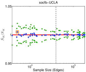
(a) Edges

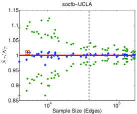
(b) Triangles

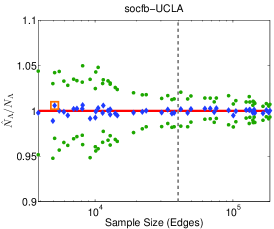
(c) Path len.2

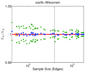
(d) Edges

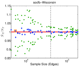
(e) Triangles

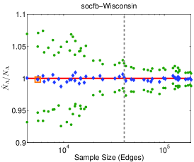
(f) Path len.2

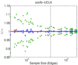
(g) Clust.

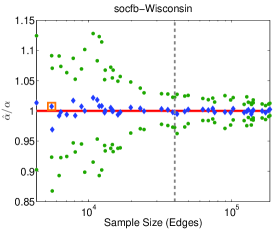
(h) Clust.

Figure 1: Convergence of the estimates ($N_{K}$, $N_{T}$, $N_{\Lambda}$, $\alpha$, upper and lower bounds) for socfb-UCLA and socfb-Wisconsin graphs, for all possible samples with $p,q$ in the range $0.005$–$0.1$. Diamonds (Blue): $\frac{E(est)}{Actual}$. Circles (Green): $\frac{UB}{Actual},\frac{LB}{Actual}$. Square (Gold): refers to the sample in Table 3. Dashed line (Grey): refers to the sample with sample size = 40K edges

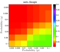
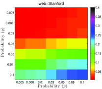
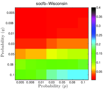
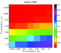
Figure 2: Sampling Fraction ($\frac{SSize}{m}$, where $SSize$ is the number of sampled edges) as $p,q$ changes in the range $0.005$–$0.1$ for web-Google, web-Stanford, socfb-Wisconsin, and socfb-CMU graphs (ordered from sparse $\rightarrow$ dense).

5.2 Confidence Bounds

Having selected a sample that can be used to estimate the actual statistic, it is also desirable to construct a confidence interval within which we are sufficiently sure that the actual graph statistic of interest lies. We construct a $95$% confidence interval for the estimates for edge ($N_{K}$), triangle ($N_{T}$), connected paths of length 2 ($N_{\Lambda}$) counts, and clustering coefficient ($\alpha$) as follows,

$$est\pm 1.96\sqrt{Var(est)}$$ (24)

where the estimates $est$ and $Var(est)$ are computed using the equations of the unbiased estimators of counts and their variance as discussed in Section 2. For example, the $95$% confidence interval for the edge count is,

$$\widehat{N}_{K}\pm 1.96\sqrt{Var(\widehat{N}_{K})}$$ (25)

where $UB=\widehat{N}_{K}+1.96\sqrt{Var(\widehat{N}_{K})}$, $LB=\widehat{N}_{K}-1.96\sqrt{Var(\widehat{N}_{K})}$ are the upper and lower bounds on the edge count respectively. Table 3 provides the $95$% upper and lower bounds (i.e., $UB,LB$) for the sample when the sample size is $\leq 40K$ edges. We observe that the actual statistics across all different graphs lie in between the bounds of the confidence interval (i.e., $LB\leq Actual\leq UB$).

Additionally, we study the properties of the sampling distribution of our proposed framework (gSH) as we change the sample size. Figure 1 shows the sampling distribution as we increase the sample size (for all possible settings of $p,q$ in the range $0.005$–$0.1$ as described previously). More specifically, we plot the fraction $\frac{E(est)}{Actual}$ (blue diamonds in the figure), where $E(est)$ is the mean estimated value across $100$ independent runs. Further, we plot the fractions $\frac{UB}{Actual}$, and $\frac{LB}{Actual}$ (green circles in the figure). These plots show the sampling distribution of all statistics for socfb-UCLA, and socfb-Wisconsin graphs. We now summarize our findings from Figure 1:

• We observe that the sampling distribution is centered and balanced over the red line ($y_{axis}=1$) which represents the actual value of the graph statistic. This observation shows the unbiased properties of the estimators for the four graph quantities of interest that we discussed in Section 2.

• We observe that the upper and lower bounds contain the actual value (represented by the red line) for different combinations of $p,q$

• We observe that as we increase the sample size, the bounds converge to be more concentrated over the actual value of the graph statistic (i.e, variance is decreasing)

• We observe that the confidence intervals for edge counts are small in the range of $0.98$–$1.02$

• We observe that the confidence intervals for triangle counts and clustering coefficient are large compared to other graph statistics (in the range of $0.87$–$1.12$).

• We observe that samples with size $=40K$ edges provide a reasonable tradeoff between the sample size and unbiased estimates with low variance

• Thus we conclude that the sampling distribution of the proposed framework has many desirable properties of unbiasedness and low variance as we increase the sample size.

Note that in Figure 1, we use a square (with gold color) to refer to the sample reported in Table 3. We also found similar observations for the remaining graphs (omitted due to space constraints).

In addition to the analysis above, we compute the exact coverage probability $\gamma$ of the $95$% confidence as follows,

$$\gamma=P(LB\leq Actual\leq UB)$$ (26)

For each $p=p_{i},q=q_{i}$, we compute the proportion of samples in which the actual statistic lies in the confidence interval across $100$ independent sampling experiments $gSH_{T}(p_{i},q_{i})$. We vary $p,q$ in the range of $0.005$–$0.01$, and for each possible combination of $p,q$ (e.g., $p=0.005,q=0.008$), we compute the exact coverage probability $\gamma$. Table 5 provides the mean coverage probability with $p,q=\{0.005,0.008,0.01\}$ for all different graphs. Note $\gamma_{N_{K}}$, $\gamma_{N_{T}}$, $\gamma_{N_{\Lambda}}$, and $\gamma_{\alpha}$ indicate the exact coverage probability of edge, triangle, path length 2 counts, and clustering coefficient respectively. We see that the nominal $95$% confidence interval holds to a good approximation, as $\gamma\approx 95$% across all graphs.

Table 4: Coverage Probability $\gamma$ for $95$% confidence interval

graph	$\gamma_{N_{K}}$		$\gamma_{N_{T}}$		$\gamma_{N_{\Lambda}}$		$\gamma_{\alpha}$
socfb-CMU	0.94		0.95		0.96		0.92
socfb-UCLA	0.96		0.95		0.95		0.92
socfb-Wisconsin	0.95		0.95		0.96		0.95
web-Stanford	0.97		0.92		0.95		0.92
web-Google	0.95		0.93		0.95		0.95
web-BerkStan	0.96		0.94		0.93		0.93

Table 5: The relative error and sample size of Jha [25] in comparison to our framework for triangle count estimation

	Jha et al. [25]		gSH
graph	$\frac{|\widehat{N}_{T}-N_{T}|}{N_{T}}$	$SSize$	$\frac{|\widehat{N}_{T}-N_{T}|}{N_{T}}$	$SSize$
web-Stanford	$\approx 0.07$	40K	0.0023	14.8K
web-Google	$\approx 0.04$	40K	0.0029	25.2K
web-BerkStan	$\approx 0.12$	40K	0.0063	39.8K

5.3 Comparison to Previous Work

We compare to the most recent research done on triangle counting by Jha et al. [25]. Jha et al.proposed a Streaming-Triangles algorithm to estimate the triangle counts. Their algorithm maintains two data structures. The first data structure is the edge reservoir and used to maintain a uniform random sample of edges as they streamed in. The second data structure is the wedge (path length two) reservoir and used to select a uniform sample of wedges created by the edge reservoir. The algorithm proceeds in a reservoir sampling fashion as a new edge $e_{t}$ is streaming in. Then, edge $e_{t}$ gets the chance to be sampled and replace a previously sampled edge with probability $1/t$. Similarly, a randomly selected new wedge (formed by $e_{t}$) replaces a previously sampled wedge from the wedge reservoir. Table 5 provides a comparison between our proposed framework (gSH) and the Streaming-Triangles algorithm proposed in  [25]. Note that we compare with the results reported in their paper.

From Table 5, we observe that across the three web graphs, our proposed framework has a relative error orders of magnitude less than the Streaming-Triangles algorithm proposed in  [25], as well as with a small(er) overhead storage (in most of the graphs). We note that the work done by Jha et al. [25] compares to other state of the art algorithms and shows that they are not practical and produce a very large error; see Section 6 for more details.

5.4 Effect of $p,q$ on Sampling Rate

While Figure 1 shows that the sampling distribution of the proposed framework is unbiased regardless the choice of $p,q$, the question of what is the effect of the choice of $p,q$ on the sample size still needs to be explored. In this section, we study the effect of the choice of parameter settings on the fraction of edges sampled from the graph.

Figure 2 shows the fraction of sampled edges as we vary $p,q$ in the range of $0.005$–$0.1$ for two web graphs and two social Facebook graphs. Note that the graphs are ordered by their density (check Table 2) going from the most sparse to the most dense graph. We observe that when $q\leq 0.01$, regardless the choice of $p$, the fraction of sampled edges is in the range of $0.5$% – $2.5$% of the total number of edges in the graph. We also observe that as $q$ goes from $0.01$ to $0.03$, the fraction of sampled edges would be in the range of $2.75$% – $5$%. These observations hold for all the graphs we studied.

On the other hand, as $q$ goes from $0.03$ to $0.1$, the fraction of sampled edges depends on whether the graph is dense or sparse. For example, for web-Google graph, as $q$ goes from $0.03$ to $0.1$, the fraction of sampled edges goes from $5$% to $15$%. Also, for web-Stanford graph, as $q$ goes from $0.03$ to $0.1$, the fraction of sampled edges goes from $5$% to $25$%. Moreover, for the most dense graph we have in this paper (socfb-CMU), the fraction of sampled edges goes from $5$% to $31$%. Note that when we tried $q=1$, regardless the choice of $p$, at least more than $80$% of the edges were sampled.

Since $p$ is the probability of sampling a fresh edge (not adjacent to a previously sampled edge), one could think of $p$ as the probability of random jumps (similar to random walk methods) to explore unsampled regions in the graph. On the other hand, $q$ is the probability of sampling an edge adjacent to previous edges. Therefore, one could think of $q$ as the probability of exploring the neighborhood of previously sampled edges (similar to the forward probability in Forest Fire sampling [29]).

From all the discussion above, we conclude that using a small $p,q$ settings (i.e., $\leq 0.008$) is better to control the fraction of sampled edges, and also recommended since the sampling distribution of the proposed framework is unbiased regardless the choice of $p,q$ as we show in Figure 1 (also see Section 2). However, if a tight confidence interval is needed, then increasing $p,q$ helps reduce the variance estimates.

Table 6: Elapsed time (seconds) for counting edges, triangles, and paths of len.2

	Full Graph		Sampled Graph
graph	Time	Graph size	Time	SSize
web-Stanford	19.68	1.9M	0.13	14.8K
web-Google	5.05	4.3M	0.55	25.2K
web-BerkStan	113.9	6.6M	1.05	39.8K

5.5 Implementation Issues

In practice, statistical variance estimators are costly to compute. In this paper, we provide an efficient parallel procedure to compute the variance estimate. We take triangles as an example. Consider for example any pair of triangles $\tau$ and $\tau^{\prime}$, assuming $\tau$ and $\tau^{\prime}$ are not identical, the covariance of $\tau$ and $\tau^{\prime}$ is greater than zero, if and only if the two triangles are intersecting. Since two intersecting triangles have either one edge in common or are identical, we can find intersecting triangles by finding all triangles incident to a particular edge $e$. In this case, the intersection probability of the two triangles is $P(\tau\cap\tau^{\prime})=P(e)$. Note that if $\tau$ and $\tau^{\prime}$ are identical, then the computation is straightforward.

The procedure is very simple as follows,

• Given a sample set of edges $\widehat{K}$, for each edge $e\in\widehat{K}$

  • find the set of all triangles ($T_{e}$) incident to $e$

  • for each pair $(\tau,\tau^{\prime})$, where $\tau,\tau^{\prime}\in T_{e}$. Compute the $Cov(\tau,\tau^{\prime})$ such that $P(\tau\cap\tau^{\prime})=P(e)$

Since, the computation of each edge is independent of other edges, we parallelize the computation of the variance estimators. Moreover, since the computation of triangle counts and paths of length two can themselves be parallelized, we compare the total elapsed time in seconds used to compute these counts on both the full graph and a sampled graph of size $\leq 40K$ edges. Table 6 provide the results of this comparison for the three web graphs. Note that in the case of the sampled graph, we also sum the computations of the variance estimators in addition to the triangle and paths of length two count estimators. Also, note that we use the sample reported in Table 3. The results show a significant reduction in the time needed to compute triangles and paths of length two counts. For example, consider the web-BerkStan graph, where the total time is reduced from 113 seconds to 1.05 seconds. Note that all the computations of Table 6 are performed on a Macbook Pro laptop 2.9GHZ Intel Core i7 with 8GB memory. Note that the storage state of gSH is only in terms of the number of sampled edges. In others words, the storage of the sampling probabilities is negligible since it is not part of the in-memory consulting state of the stream sampling framework gSH. Moreover, we use only three different probabilities, ($p,q$ and $1$), that can be stored with a custom $2-bit$ data structure, where $00$, $01$, and $10$ represents $p,q$ and $1$ respectively.

6 Related Work

In this section, we discuss the related work on the problem of large-scale graph analytics and their applications. Generally speaking, there are two bodies of work related to this paper: (i) graph analytics in graph stream setting, and (ii) graph analytics in the non-streaming setting (e.g. using MapReduce and Hadoop). In this paper, we propose a generic stream sampling framework for big-graph analytics, called Graph Sample and Hold (gSH), that works in a single pass over the streams. Therefore, we focus on the related work for graph analytics in graph stream setting and we briefly review the other related work.

Graph Analysis Using Streaming Algorithms

Before exploring the literature of graph stream analytics, we briefly review the literature in data stream analysis and mining that may not contain graph data. For example, for sequence sampling (e.g., reservoir sampling) [47, 6], for computing frequency counts [32, 12] and load shedding [43], and for mining concept drifting data streams [20]. Additionally, The idea of sample and hold (SH) was introduced in [19] for unbiased sampling of network measurements with integral weights. Subsequently, other work explored adaptive SH, and SH with signed updates [14, 15]. Nevertheless, none of this work has considered the framework of sample and hold (SH) for social and information networks. In this paper, however, we propose the framework of graph sample and hold (gSH) for big-graph analytics.

There has been an increasing interest in mining, analysis, and querying of massive graph streams as a result of the proliferation of graph data (e.g., social networks, emails, IP traffic, Twitter hashtags). Following the earliest work on graph streams [23], several types of problems were explored in the field of analytics of massive graph streams. For example, to count triangles [25, 34, 8, 11, 9, 26], finding common neighborhoods [10], estimating pagerank values [36], and characterizing degree sequences in multi-graph streams [16]. In the data mining and machine learning field, there is the work done on clustering graph streams [2], outlier detection [3], searching for subgraph patterns [13], mining dense structural patterns [1], and querying the frequency of particular edges and subgraphs in the graphs streams [50]. For an excellent survey on analytics of massive graph streams, we refer the reader to [33, 49].

Much of this work has used various sampling schemes to sample from the stream of graph edges. Surprisingly, the majority of this work has focused primarily on sampling schemes that can be used to estimate certain graph properties (e.g. triangle counts), while much less is known for the case when we need a generic approach to estimate various graph properties with the same sampling scheme with minimum assumptions.

For example, the work done in [11] proposed an algorithm with space bound guarantees for triangle counting and clustering estimation in the incidence stream model where all edges incident to a node arrive in order together. However, in the incidence stream model, counting triangles is a relatively easy problem, and counting the number of paths of length two is simply straightforward. On the other hand, it has been shown that these bounds and accurate estimates will no longer hold in the case of adjacency stream model, where the edges arrive arbitrarily with no particular order [25, 34].

Another example, the work done Jha et al.in [25] proposed a practical, single pass, $O(\sqrt{n})$-space streaming algorithm specifically for triangle counting and clustering estimation with additive error guarantee (as opposed to other algorithms with relative error guarantee). Although, the algorithm is practical and approximates the triangle counts accurately at a sample size of $40K$ edges, their method is specifically designed for triangle counting. Nevertheless, we compare to the results of triangle counts reported in [25], and we show that our framework is not only generic but also produces errors with orders of magnitude less than the algorithm in [25], and with a small(er) storage overhead in many times.

More recently, Pavan et al.proposed a space-efficient streaming algorithm for counting and sampling triangles in [34]. This algorithm is practical and works in a single pass streaming fashion with order $O(m\Delta/T)$-space, where $\Delta$ is the maximum degree of the graph. However, this algorithm needs to store estimators (i.e., wedges that may form potential triangles), and each of these estimators stores at least one edge. In their paper, the authors show that they need at least $128$ estimators (i.e., more than $128K$ edges), to obtain accurate results (large storage overhead compared to this paper). The sampling algorithm of [34] bears some formal resemblance to our approach in using different sampling probabilities depending on whether or not an arriving edge is adjacent to a previous edge, but otherwise the details are substantially different.

Other semi-streaming algorithms were proposed for triangle counting, such as the work in [9], however, they are not practical and produce large error as discussed in [34].

Horvitz-Thompson estimation was proposed in the graphical setting by Frank [21], including applications to subgraph sampling, but limited to a model of simple random sampling of vertices without replacement; see also Kolaczyk [27].

Graph Analysis Using Static and Parallel Algorithms

We briefly review other research for graph analysis in non-streaming setting (i.e., static). For example, exact counting of triangles with runtime ($O(m^{3/2}$) [37], or approximately by sampling edges as in [45]. Although not working in a streaming fashion, the algorithm in [45] uses unbiased estimators of triangle counts similar to our work. Moreover, other algorithms were proposed based on wedge sampling and proved to be accurate in practice, such as the work in [39, 40, 28]. More recently, the work done in [35] proposed a parallel framework for finding the maximum clique.

Finally, there has been an increasing interest in the general problem of network sampling. For example, to obtain a representative subgraph [29, 4], to preserve the community structure [30, 31], to perform A/B testing of social features [7], and many other interesting work [17, 5, 46].

7 Conclusion

In this paper, we presented a generic framework for big-graph analytics called graph sample and hold (gSH). The gSH framework samples from massive graphs sequentially in a single pass, one edge at a time, while maintaining a small state typically less than $1$% of the total number of edges in the graph. Our contributions can be summarized in the following points:

• gSH works sequentially in a single pass, while maintaining a small state.

• We show how to produce unbiased estimators and their variance for four specific graph quantities of interest to estimate within the framework. Further, we show how to obtain confidence bounds using the variance unbiased estimators.

• We conducted several experiments on real world graphs, such as social Facebook graphs, and web graphs. The results show that the relative error goes from $0.02$% to $0.95$% for a sample with $\leq 40K$ edges, across different types of graphs. Moreover, the results show that the sampling distribution is centered and balanced over the actual values of the four graph quantities of interest, with tightening error bounds as the sample size increases.

• We discuss the effect of parameter choice $p,q$ on the proportion of sampled edges.

• We compare to the state of the art [25], and our proposed framework has a relative error orders of magnitude less than the Streaming-Triangles algorithm proposed in  [25], as well as with a small(er) overhead storage (in most of the graphs). We note that the work in [25] compares to other state of the art algorithms and shows that they are not practical and produce a very large error; see Section 6 for more details.

• We show how to parallelize and efficiently compute the unbiased variance estimators, and we discuss the significant reductions in computation time that can be achieved by gSH framework.

In future work, we aim to extend gSH to other graph properties, such as cliques, coloring number, and size of connected components, among many others.

References

- [1] Aggarwal, C., Li, Y., Yu, P., and Jin, R. On dense pattern mining in graph streams. Proceedings of the VLDB Endowment 3, 1-2 (2010), 975–984.
- [2] Aggarwal, C., Zhao, Y., and Yu, P. On clustering graph streams. In SDM (2010), pp. 478–489.
- [3] Aggarwal, C., Zhao, Y., and Yu, P. Outlier detection in graph streams. In ICDE (2011), pp. 399–409.
- [4] Ahmed, N. K., Neville, J., and Kompella, R. Network sampling: from static to streaming graphs. to appear in TKDD. arXiv:1211.3412 (2012).
- [5] Al Hasan, M., and Zaki, M. Output space sampling for graph patterns. Proceedings of the VLDB Endowment 2, 1 (2009), 730–741.
- [6] Babcock, B., Datar, M., and Motwani, R. Sampling from a moving window over streaming data. In SODA (2002), pp. 633–634.
- [7] Backstrom, L., and Kleinberg, J. Network bucket testing. In WWW (2011), pp. 615–624.
- [8] Bar-Yossef, Z., Kumar, R., and Sivakumar, D. Reductions in streaming algorithms with an application to counting triangles in graphs. In SODA (2002), pp. 623–632.
- [9] Becchetti, L., Boldi, P., Castillo, C., and Gionis, A. Efficient semi-streaming algorithms for local triangle counting in massive graphs. In Proc. of KDD (2008), pp. 16–24.
- [10] Buchsbaum, A., Giancarlo, R., and Westbrook, J. On finding common neighborhoods in massive graphs. Theoretical Computer Science 299, 1 (2003), 707–718.
- [11] Buriol, L., Frahling, G., Leonardi, S., Marchetti-Spaccamela, A., and Sohler, C. Counting triangles in data streams. In PODS (2006), pp. 253–262.
- [12] Charikar, M., Chen, K., and Farach-Colton, M. Finding frequent items in data streams. Automata, Languages and Programming (2002), 784–784.
- [13] Chen, L., and Wang, C. Continuous subgraph pattern search over certain and uncertain graph streams. IEEE Transactions on Knowledge and Data Engineering 22, 8 (2010), 1093–1109.
- [14] Cohen, E., Cormode, G., and Duffield, N. Don’t let the negatives bring you down: sampling from streams of signed updates. In SIGMETRICS 40, 1 (2012), 343–354.
- [15] Cohen, E., Duffield, N., Kaplan, H., Lund, C., and Thorup, M. Algorithms and estimators for accurate summarization of internet traffic. In Proc. of SIGCOMM (2007), pp. 265–278.
- [16] Cormode, G., and Muthukrishnan, S. Space efficient mining of multigraph streams. In PODS (2005), pp. 271–282.
- [17] Dasgupta, A., Kumar, R., and Sivakumar, D. Social sampling. In SIGKDD (2012), pp. 235–243.
- [18] Estan, C., and Varghese, G. New directions in traffic measurement and accounting. In Proc. ACM SIGCOMM ’2002 (Pittsburgh, PA, Aug. 2002).
- [19] Estan, C., and Varghese, G. New directions in traffic measurement and accounting. In Proc. of SIGCOMM (2002), pp. 323–336.
- [20] Fan, W. Streamminer: a classifier ensemble-based engine to mine concept-drifting data streams. In VLDB (2004), pp. 1257–1260.
- [21] Frank, O. Sampling and estimation in large social networks. Social Networks 1, 1 (1978), 91–101.
- [22] Gibbons, P., and Matias, Y. New sampling-based summary statistics for improving approximate query answers. In SIGMOD (1998), ACM.
- [23] Henzinger, M., Raghavan, P., and Rajagopalan, S. Computing on data streams. In External Memory Algorithms: Dimacs Workshop External Memory and Visualization (1999), vol. 50, p. 107.
- [24] Horvitz, D. G., and Thompson, D. J. A generalization of sampling without replacement from a finite universe. Journal of the American Statistical Association 47, 260 (1952), 663–685.
- [25] Jha, M., Seshadhri, C., and Pinar, A. A space efficient streaming algorithm for triangle counting using the birthday paradox. In In ACM SIGKDD (2013), pp. 589–597.
- [26] Jowhari, H., and Ghodsi, M. New streaming algorithms for counting triangles in graphs. In Computing and Combinatorics. Springer, 2005, pp. 710–716.
- [27] Kolaczyk, E. Statistical analysis of network data, 2009.
- [28] Kolda, T. G., Pinar, A., Plantenga, T., Seshadhri, C., and Task, C. Counting triangles in massive graphs with mapreduce. arXiv:1301.5887 (2013).
- [29] Leskovec, J., and Faloutsos, C. Sampling from large graphs. In SIGKDD (2006), pp. 631–636.
- [30] Maiya, A. S., and Berger-Wolf, T. Y. Sampling Community Structure. In WWW (2010), pp. 701–710.
- [31] Maiya, A. S., and Berger-Wolf, T. Y. Benefits of bias: Towards better characterization of network sampling. In SIGKDD (2011), pp. 105–113.
- [32] Manku, G. S., and Motwani, R. Approximate Frequency Counts over Data Streams. In VLDB (2002), pp. 346–357.
- [33] McGregor, A. Graph mining on streams. Encyclopedia of Database Systems (2009), 1271–1275.
- [34] Pavan, A., Tangwongsan, K., Tirthapura, S., and Wu, K.-L. Counting and sampling triangles from a graph stream. Proc. of VLDB 6, 14 (2013), 1870–1881.
- [35] Rossi, R. A., Gleich, D. F., Gebremedhin, A. H., and Patwary, M. A. Fast maximum clique algorithms for large graphs. In Proc. of WWW (2014).
- [36] Sarma, A. D., Gollapudi, S., and Panigrahy, R. Estimating PageRank on Graph Streams. In PODS (2008), pp. 69–78.
- [37] Schank, T. Algorithmic aspects of triangle-based network analysis.
- [38] Schervish, M. J. Theory of Statistics. Springer, 1995.
- [39] Seshadhri, C., Pinar, A., and Kolda, T. G. Fast triangle counting through wedge sampling. In Proc. of SIAM (2013).
- [40] Seshadhri, C., Pinar, A., and Kolda, T. G. Wedge sampling for computing clustering coefficients and triangle counts on large graphs. arXiv:1309.3321 (2013).
- [41] Smitha, Kim, I., and Reddy, A. Identifying long term high rate flows at a router. In in Proc. of High Performance Computing (December 2001).
- [42] SNAP. http://snap.stanford.edu/data/index.html, 2014.
- [43] Tatbul, N., Çetintemel, U., Zdonik, S., Cherniack, M., and Stonebraker, M. Load shedding in a data stream manager. In VLDB (2003), pp. 309–320.
- [44] Traud, A. L., Mucha, P. J., and Porter, M. A. Social structure of facebook networks. Physica A: Statistical Mechanics and its Applications 391, 16 (2012), 4165–4180.
- [45] Tsourakakis, C. E., Kang, U., Miller, G. L., and Faloutsos, C. Doulion: counting triangles in massive graphs with a coin. In Proc. of KDD (2009), pp. 837–846.
- [46] Vattani, A., Chakrabarti, D., and Gurevich, M. Preserving personalized pagerank in subgraphs. In ICML (2011).
- [47] Vitter, J. Random sampling with a reservoir. ACM Trans. Math. Softw. 11 (1985).
- [48] Williams, D. Probability with Martingales. Cambridge University Press, 1991.
- [49] Zhang, J. A survey on streaming algorithms for massive graphs. Managing and Mining Graph Data (2010), 393–420.
- [50] Zhao, P., Aggarwal, C. C., and Wang, M. gsketch: On query estimation in graph streams. Proc. of VLDB 5, 3 (2011), 193–204.