Efficient Computation of Visibility Polygons

Abstract

Determining visibility in planar polygons and arrangements is an important subroutine for many algorithms in computational geometry. In this paper, we report on new implementations, and corresponding experimental evaluations, for two established and one novel algorithm for computing visibility polygons. These algorithms will be released to the public shortly, as a new package for the Computational Geometry Algorithms Library (CGAL).

1 Introduction

Visibility is a basic concept in computational geometry. For a polygon $P\subset\mathds{R}^{2}$, we say that a point $p\in P$ is visible from $q\in P$ if the line segment $\overline{pq}\subseteq P$. The points that are visible from $q$ form the visibility region $\mathcal{V}(q)$. Usually (if no degeneracies occur) $\mathcal{V}(q)$ is a polygon; hence it is often called the visibility polygon. If there are multiple vertices collinear with $q$, then $\mathcal{V}(q)$ may take the form of a polygon with attached one-dimensional antennae (see Figure 1).

Computing $\mathcal{V}(q)$, given a query point $q$, is a well-known problem with a number of established algorithms; see the book by Ghosh [9]. Besides being of interest on its own, it also frequently appears as a subroutine in algorithms for other problems, most prominently in the context of the Art Gallery Problem [16]. In experimental work on this problem [15] we have identified visibility computations as having a substantial impact on overall computation times, even though it is a low-order polynomial-time subroutine in an algorithm solving an NP-hard problem. Therefore it is of enormous interest to have efficient implementations of visibility polygon algorithms available.

CGAL, the Computational Geometry Algorithms Library [6], contains a large number of algorithms and data structures, but unfortunately not for the computation of visibility polygons. We present implementations for three algorithms, which form the basis for an upcoming new CGAL package for visibility. Two of these are efficient implementations for standard $\operatorname{O}(n)$- and $\operatorname{O}(n\log n)$-time algorithms from the literature. In addition, we describe a novel algorithm with preprocessing, called triangular expansion, based on an intriguingly simple idea using a triangulation of the underlying polygon. Even though this algorithm has a worst-case query runtime of $\operatorname{O}(n^{2})$, it is extremely fast in practice. In experiments we have found it to outperform the other implementations by about two orders of magnitude on large and practically relevant inputs. The implementations follow the exact computation paradigm and handle all degenerate cases, whether or not to include antennae in the output is configurable. Such a visibility polygon $\mathcal{V}(q)$ with antenna $bc$ is depicted on in the figure to the right.

Our contribution is therefore threefold: We present a new algorithm for computing visibility polygons. We report on an experimental evaluation, demonstrating the efficiency of the implementations, and revealing superior speed of the novel algorithm. The publication of the code is scheduled for CGAL release 4.5 (October 2014).

2 Related Work

For a detailed coverage of visibility algorithms in two dimensions, see the book [9]. We denote by $n$ the number of vertices of the input polygon $P$, by $h$ the number of its holes, and by $k$ the complexity of the visibility region $\mathcal{V}(q)$ of the query point $q$.

The problem of computing $\mathcal{V}(q)$ was first addressed for simple polygons in [8]. The first correct $O(n)$ time algorithm was given by Joe and Simpson [14]. For a polygon with holes, $O(n\log n)$ time algorithms were proposed by Suri et al. [17] and Asano et al. [3]. An optimal $O(n+h\log h)$ algorithm was later given by Heffernan and Mitchell [11].

Ghodsi et al. [10] reduced the query time for simple polygons to $O(\log n+k)$, at the expense of preprocessing requiring $O(n^{3})$ time and space. In [5] Bose et al. showed that this time can also be achieved for points outside of $P$ with an $O(n^{3}\log n)$ preprocessing time. Aronov et al. [1] reduced the preprocessing time and space to $O(n^{2}\log n)$ and $O(n^{2})$ respectively with the query time being increased to $O(\log^{2}n+k)$.

Allowing preprocessing for polygons with holes, Asano et al. [3] presented an algorithm with $O(n)$ query time that requires $O(n^{2})$ preprocessing time and space. Vegter [18] gave an output sensitive algorithm whose query time is $O(k\log(n/k))$, where preprocessing takes $O(n^{2}\log n)$ time and $O(n^{2})$ space. Zarei and Ghodsi [19] gave another output sensitive algorithm whose query time is $O(1+\min(h,k)\log n+k)$ with $O(n^{3}\log n)$ preprocessing time and $O(n^{3})$ space. Recent work by Inkulu and Kapoor [12] extends the approaches of [1] and [19] by incorporating a trade-off between preprocessing and query time.

Surprisingly, it seems that there are no exact and complete implementations of these algorithms at all. The only available software is GEOMPACK [13] but it does not use exact arithmetic and only implements the algorithm for simple polygons of Joe and Simpson [14].

3 Implemented Algorithms

The following algorithms are implemented in C++, and are part of an upcoming CGAL package for visibility.

3.1 Algorithm of Joe and Simpson [14]

The visibility polygon algorithm by Joe and Simpson [14] runs in $O(n)$ time and space. It performs a sequential scan of the boundary of $P$, a simple polygon (without holes), and uses a stack $s$ of boundary points $s_{0},s_{1},\ldots,s_{t}$ such that at any time, the stack represents the visibility polygon with respect to the already scanned part of $P$’s boundary.

When the current edge $v_{i}v_{i+1}$ is in process, three possible operations can be performed: new boundary points are added to the stack, obsolete boundary points are deleted from the stack, or subsequent edges on the polygon’s boundary are scanned until a certain condition is met. The later is performed when the edge enters a so-called “hidden-window,” where the points are not visible from the viewpoint $q$.

The implementation uses states to process the boundary of the polygon $P$ and manipulate the stack $s$ such that, in the end, it contains the vertices defining the visibility polygon’s boundary. The main state handles the case when the current edge $v_{i}v_{i+1}$ takes a left turn and $v_{i+1}$ is pushed on the stack. The other states are entered when $v_{i}v_{i+1}$ turns behind a previous edge. Then the algorithm scans the subsequent edges until the boundary reappears from behind the last visible edge. In order to deal with cases in which the polygon winds more than $360^{\circ}$, a winding counter is used during this edge processing.

3.2 Algorithm of Asano [2]

The algorithm by Asano [2] runs in $O(n\log n)$ time and $O(n)$ space. It follows the classical plane sweep paradigm with the difference that the event line $L$ is a ray that originates from and rotates around the query point $q$. Thus, initially all vertices of the input polygon (event points) are sorted according to their polar angles with respect to the query point $q$. Segments that intersect the ray $L$ are stored in a balanced binary tree $T$ based on their order of intersections with $L$. As the sweep proceeds, $T$ is updated and a new vertex of $V(q)$ is generated each time the smallest element (segment closest to $q$) in $T$ changes.

The algorithm can be implemented using basic algorithms and data structures such as std::sort (for ordering event points) and std::map (ordering segments on the ray). However, it is crucial that the underlying comparison operations are efficient. We omit details of the angular comparison for vertices and sketch the ordering along $L$.

For an efficient comparison of two segments $s_{1}$ and $s_{2}$ along the ray $L$, it is important to avoid explicit (and expensive) construction of intersection points with $L$. In fact, $L$ can stay completely abstract. Assuming that $s_{1}$ and $s_{2}$ have no common endpoint, the order can be determined using at most five orientation predicates. Consider the figure to the right: the segment $s_{1}$ is further away since $q$, $a_{2}$ and $b_{2}$ are on the same side of $s_{1}$ (three calls). In case this is not conclusive, two additional calls for $q$ and $a_{1}$ with respect to $s_{2}$ are sufficient.

3.3 New Algorithm: Triangular Expansion

We introduce a new algorithm that, to the best of our knowledge, has not been discussed in the literature. Its worst case complexity is $O(n^{2})$ but it is very efficient in practice as it is, in some sense, output sensitive.

In an initial preprocessing phase the polygon is triangulated. For polygons with holes this is possible in $O(n\log n)$ time [4] and in $O(n)$ time for simple polygons [7]. However, for the implementation we used CGAL’s constrained Delaunay triangulation which requires $O(n^{2})$ time in the worst case but behaves well in practice.

Given a query point $q$, we locate the triangle containing $q$ by a simple walk. Obviously $q$ sees the entire triangle and we can report all edges of this triangle that belong to $\partial P$. For every other edge we start a recursive procedure that expands the view of $q$ through that edge into the next triangle. Initially the view is restricted by the two endpoints of the edge. However, while the recursion proceeds the view can be further restricted. This is depicted in Figure 1: The recursion enters triangle $\Delta$ through edge $e$ with endpoints $a$ and $b$. The view of $q$ is restricted by the two reflex vertices $l$ and $r$, where $a\leq r<\ell\leq b$ with respect to angular order around $q$. The only new vertex is $v$ and its position with respect to $\ell$ and $r$ is computed with two orientation tests. In the example of Figure 1 the vertex $v$ is between $\ell$ and $r$, thus we have to consider both edges $e_{\ell}$ and $e_{r}$: $e_{\ell}$ is a boundary edge and we can report edge $\overline{\ell\ell^{\prime}}$ and $\overline{\ell^{\prime}v}$ as part of $\partial{\mathcal{V}(q)}$; $e_{r}$ is not a boundary edge, which implies that the recursion continues with $v$ being the vertex that now restricts the left side of the view.

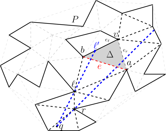
Figure 1: Triangular expansion algorithm — recursion entering triangle $\Delta$ through edge $e$.

The recursion may split into two calls if $e_{\ell}$ and $e_{r}$ are both not part of the boundary. As there are $n$ vertices, this can happen $O(n)$ times; each call may reach $O(n)$ triangles, which suggests a worst-case runtime of $O(n^{2})$. However, a true split into two visibility cones that may reach the same triangle independently can happen only at a hole of $P$. Thus, at worst the runtime is $O(nh)$, where $h$ is the number of holes. This implies that the runtime is linear for simple polygons.

Figure 2 sketches the worst case scenario, which we also used in our experiments (Section 4). The $k=\Theta(n)$ holes in the middle of the long room split the view of $v_{0}$ into $k+1$ cones, each of which passes through $k=\Theta(n)$ Delaunay edges. Thus, in this scenario the algorithm has complexity $\Theta(n^{2})$.

Figure 2: $\Theta(n^{2})$ worst case for triangular expansion.

However, ignoring the preprocessing, the algorithm often runs in sublinear time, since it processes only those triangles that are actually seen. This can be a very small subset of the actual polygon. Unfortunately, this is not strictly output sensitive, since a visibility cone may traverse a triangle even though the triangle does not contribute to the boundary of $\mathcal{V}(q)$.

Since the triangulation has linear size and since at any time there are at most $O(n)$ recursive calls on the stack, the algorithm requires $O(n)$ space.

4 Experiments

The experiments were run on an Intel(R) Core(TM) i7-3740QM CPU at 2.70GHz with 6 MB cache and 16 GB main memory running a 64-bit Linux 3.2.0 kernel. All algorithms are developed against the latest release (i.e., 4.3) of CGAL. None of the algorithms uses parallelization. We tested three different scenarios: Norway (Figure 3) a simple polygon with $20981$ vertices, cathedral (Figure 4) a general polygon with 1209 vertices, and the already mentioned worst case scenario (Figure 2) for the triangular expansion algorithm.

In tables $T_{Queries}$ indicates the total time to compute the visibility polygons for all vertices, while $T_{total}$ also includes the time for preprocessing. $Avg$ indicates the average time required to compute the visibility area for one vertex including preprocessing. Algorithms are indicated as follows: (S) the algorithm of Joe and Simpson [14] for simple polygons; (R) the algorithm of Asano [2] performing the rotational sweep around the query point; (T) our new triangular expansion algorithm.

Since runtimes did not differ significantly we do not report on similar benchmarks with query points on edges and in the interior polygon.

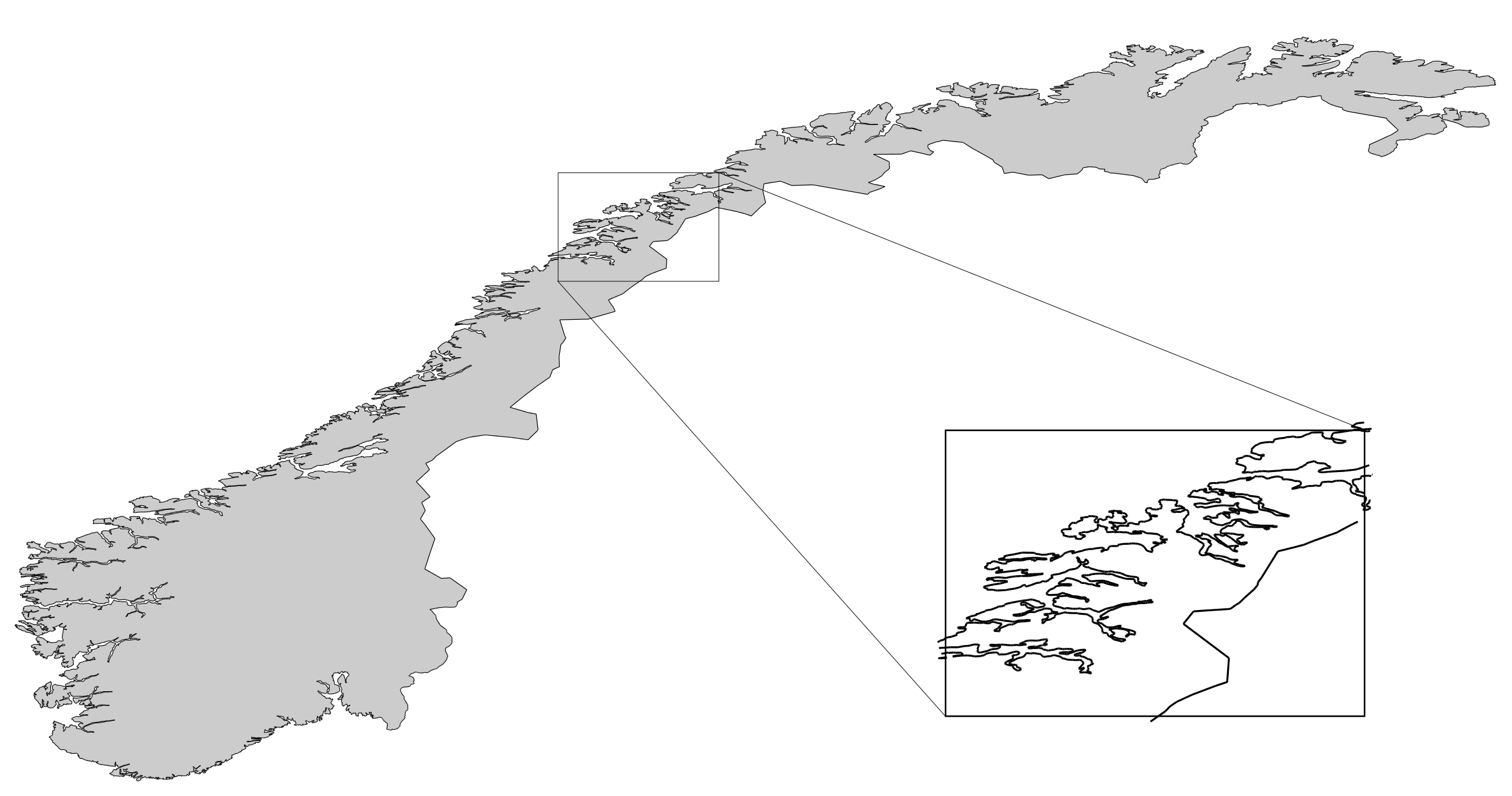
Alg.	$T_{\mbox{\scriptsize\em PrePro}}$	$T_{\mbox{\scriptsize\em Queries}}$	$T_{\mbox{\scriptsize\em Total}}$	Avg
S	—	117.43 s	117.43 s	5.60 ms
R	—	1193.29 s	1193.29 s	56.87 ms
T	0.21 s	3.66 s	3.88 s	0.18 ms

Figure 3: Norway example.

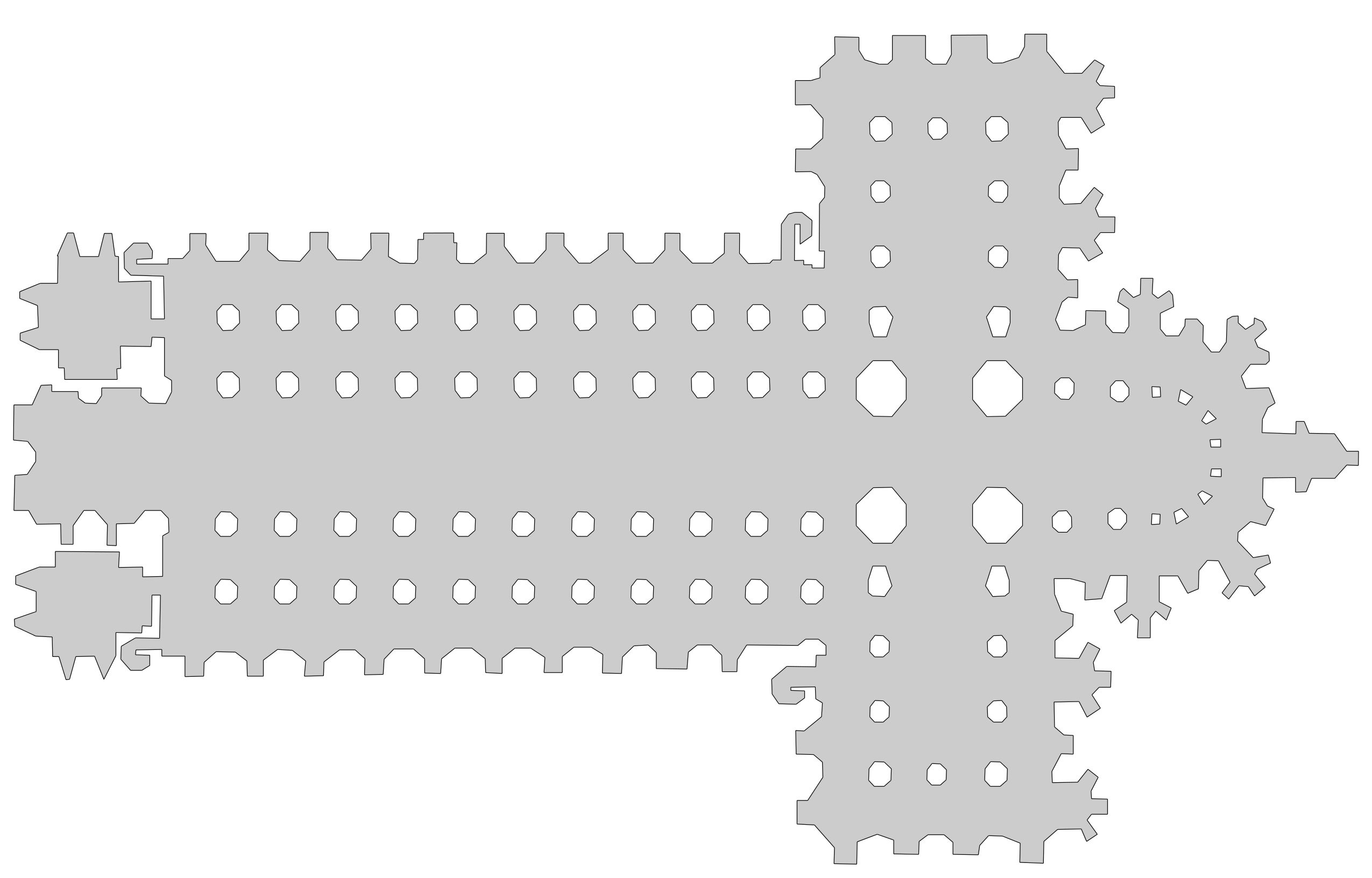
Alg.	$T_{\mbox{\scriptsize\em PrePro}}$	$T_{\mbox{\scriptsize\em Queries}}$	$T_{\mbox{\scriptsize\em Total}}$	Avg
R	—	1.35 s	1.35 s	1.112 ms
T	0.004 s	0.04 s	0.04 s	0.004 ms

Figure 4: Cathedral example.

For the real world scenarios, cathedral and Norway, we can observe that the average runtime of the triangular expansion algorithm is two orders of magnitude faster than the rotational sweep algorithm. It is more than one order of magnitude faster than the special algorithm for simple polygons on the Norway data set. However, for the worst case scenario, Figure 5 shows that eventually the sweep algorithm becomes faster with increasing input complexity.

Figure 5: Worst case scenario.

Acknowledgements.

This work was supported by Google Summer of Code and the Deutsche Forschungsgemeinschaft (DFG), contract KR 3133/1-1 (Kunst!).

References

- [1] B. Aronov, L. J. Guibas, M. Teichmann, and L. Zhang. Visibility queries and maintenance in simple polygons. Discrete & Comp. Geometry, 27(4):461–483, 2002.
- [2] T. Asano. An efficient algorithm for finding the visibility polygon for a polygonal region with holes. IEICE Transactions, 68(9):557–559, 1985.
- [3] T. Asano, T. Asano, L. Guibas, J. Hershberger, and H. Imai. Visibility of disjoint polygons. Algorithmica, 1(1-4):49–63, 1986.
- [4] M. de Berg, O. Cheong, M. van Kreveld, and M. Overmars. Computational Geometry: Algorithms and Applications. Springer-Verlag, 3rd edition, 2008.
- [5] P. Bose, A. Lubiw, and J. I. Munro. Efficient visibility queries in simple polygons. Computational Geometry, 23(3):313–335, 2002.
- [6] Cgal, Computational Geometry Algorithms Library. http://www.cgal.org.
- [7] B. Chazelle. Triangulating a simple polygon in linear time. Discrete & Comp. Geom., 6(1):485–524, 1991.
- [8] L. S. Davis and M. L. Benedikt. Computational models of space: Isovists and isovist fields. Computer Graphics and Image Processing, 11(1):49–72, 1979.
- [9] S. K. Ghosh. Visibility algorithms in the plane. Cambridge University Press, 2007.
- [10] L. J. Guibas, R. Motwani, and P. Raghavan. The robot localization problem. SIAM Journal on Computing, 26(4):1120–1138, 1997.
- [11] P. J. Heffernan and J. S. Mitchell. An optimal algorithm for computing visibility in the plane. SIAM Journal on Computing, 24(1):184–201, 1995.
- [12] R. Inkulu and S. Kapoor. Visibility queries in a polygonal region. Comp. Geometry, 42(9):852–864, 2009.
- [13] B. Joe. Geompack users’ guide. Department of Computing Science, University of Alberta, Edmonton, Alberta, Canada T6G 2H1, 1993.
- [14] B. Joe and R. Simpson. Corrections to Lee’s visibility polygon algorithm. BIT Numerical Mathematics, 27(4):458–473, 1987.
- [15] A. Kröller, T. Baumgartner, S. P. Fekete, and C. Schmidt. Exact solutions and bounds for general art gallery problems. Journal of Experimental Algorithmics, 17(1), 2012.
- [16] J. O’Rourke. Art Gallery Theorems and Algorithms. International Series of Monographs on Computer Science. Oxford University Press, New York, NY, 1987.
- [17] S. Suri and J. O’Rourke. Worst-case optimal algorithms for constructing visibility polygons with holes. In Proceedings of the second annual symposium on Computational geometry, pages 14–23. ACM, 1986.
- [18] G. Vegter. The visibility diagram: a data structure for visibility problems and motion planning. In SWAT 90, pages 97–110. Springer, 1990.
- [19] A. Zarei and M. Ghodsi. Efficient computation of query point visibility in polygons with holes. In Proceedings of the twenty-first annual symposium on Computational geometry, pages 314–320. ACM, 2005.