Average Case Performance of Replicator Dynamics in Potential Games via Computing Regions of Attraction

Abstract

What does it mean to fully understand the behavior of a network of adaptive agents? The golden standard typically is the behavior of learning dynamics in potential games, where many evolutionary dynamics, e.g., replicator dynamics, are known to converge to sets of equilibria. Even in such classic settings many questions remain unanswered. We examine issues such as:

• Point-wise convergence: Does the system always equilibrate, even in the presence of continuums of equilibria?

• Computing regions of attraction: Given point-wise convergence can we compute the region of asymptotic stability of each equilibrium (e.g., estimate its volume, geometry)?

• System invariants: Invariant functions remain constant along every system trajectory. This notion is orthogonal to the game theoretic concept of a potential function, which always strictly increases/decreases along system trajectories. Do dynamics in potential games exhibit invariant functions? If so, how many? How do these functions look like?

Based on these geometric characterizations, we propose a novel quantitative framework for analyzing the efficiency of potential games with many equilibria. The predictions of different equilibria are weighted by their probability to arise under evolutionary dynamics given uniformly random initial conditions. This average case analysis is shown to offer novel insights in classic game theoretic challenges, including quantifying the risk dominance in stag-hunt games and allowing for more nuanced performance analysis in networked coordination and congestion games with large gaps between price of stability and price of anarchy.

1 Introduction

The study of game dynamics is a basic staple of game theory with several books dedicated exclusively to it [14, 12, 37, 6, 34]. Historically, the golden standard for classifying the behavior of learning dynamics in games has been to establish convergence to equilibria. Thus, it is hardly surprising that a significant part of the work on learning in games focuses on potential games (and slight generalizations thereof) where many dynamics (e.g., replicator, smooth fictitious play) are known to converge to equilibrium sets. The structure of the convergence proofs is essentially universal across different learning dynamics and boils down to identifying a Lyapunov/potential function that strictly decreases along any nontrivial trajectory. In potential games, as their name suggests, this function is part of the description of the game and precisely guides self-interested dynamics towards critical points of these functions that correspond to equilibria of the learning process.

Potential games are also isomorphic to congestion games [24]. Congestion games have been instrumental in the study of efficiency issues in games. They are amongst the most extensively studied class of games from the perspective of price of anarchy and price of stability with many tight characterization results for different subclasses of games (e.g., linear congestion games [33], symmetric load balancing [26] and references therein).

Given this extensive treatment of such a classic class of games it would seem, at a first glance, that our understanding of these systems is more or less complete. We show that this is far from the case. We focus on simple systems where replicator dynamic, arguably one of the most well studied game dynamics, is applied to linear congestion games and (network) coordination games. We resolve a number of basic open questions in the following results:

A) Point-wise convergence to equilibrium: In the case of linear congestion games and (network) coordination games we prove convergence to equilibrium instead of equilibrium sets. Convergence to equilibrium sets implies that the distance of system trajectories from the sets of equilibria converges to zero. On the other hand, convergence to equilibrium, also referred to as point-wise convergence, implies that every system trajectory has a unique limit point, which is an equilibrium. In games with continuums of equilibria, (e.g., $N$ balls $N$ bins games with $N\geq 4$), the first statement is more inclusive that the second. In fact, system equilibration is not implied by set-wise convergence, and the limit set of a trajectory may have complex topology (e.g., the limit of social welfare may not be well defined). Despite numerous positive convergence results in classes of congestion games ([11, 4, 10, 3, 1]), this is the first to our knowledge result about deterministic point-wise convergence for any concurrent dynamic. This argument is based on combining global Lyapunov functions arguments with local information theoretic Lyapunov functions around each equilibrium.

B) Global stability analysis: Although the point-wise convergence result is interesting in itself, it critically enables all other results in the paper. Specifically, we establish that modulo point-wise convergence, all but a zero measure set of initial conditions converge to equilibrium points which are (linearly) stable ($i.e.$, their Jacobian has no eigenvalue with positive real part). This is a technical result that combines game theoretic arguments with tools from dynamical systems (Center-Stable Manifold theorem) and analysis (Lindelőf’s lemma). [17] has established that all such equilibria must satisfy a refined game theoretic property and known as weakly stability. A Nash equilibrium is weakly stable if given any two randomizing agents, fixing one of the agents to choosing one of his strategies with probability one, leaves the other agent indifferent between the strategies in his support. This condition is easy to work with (does not require computing eigenvalues) and sometimes (along with the global stability result) already suffices to make a unique prediction about the resulting system performance.

C) Invariant functions: Sometimes a game may have multiple (weakly) stable equilibria. In this case we would like to be able to predict which one will arise given a specific (or maybe a randomly chosen) initial condition. Systems invariants allows us to do exactly that. A system invariant is a function defined over the system state space such that it remains constant along every system trajectory. Establishing invariant properties of replicator dynamics in generalized zero-sum games has helped prove interesting topological properties of the system trajectories such as (near) cycles [31, 32, 29]. In the case of bipartite coordination games with fully mixed Nash equilibria, we can establish similar invariant functions. Specifically, the difference between the sum of the Kullback-Leibler (K-L) divergences of the evolving mixed strategies of the agents on the left partition from their fully mixed Nash equilibrium strategy and the respective term for the agents in the right partition remains constant along any trajectory. In the special case of star graphs, we show how to produce $n$ such invariants where $n$ is the degree of the star. This allows for creating efficient oracles for predicting to which Nash equilibrium the system converges provably for any initial condition without simulating explicitly the system trajectory.

Applications: The tools that we have developed allow for novel insights in classic and well studied class of games. We group our results into two clusters, average case performance analysis and estimating risk dominance/regions of attraction.

Average Case Performance: We propose a novel quantitative framework for analyzing the efficiency of potential games with many equilibria. Informally, we define the expected system performance as the weighted average of the social costs of all equilibria where the weight of each equilibrium is proportional to the volume (or more generally measure) of its region of attraction.

The main idea is as follows: The agents start participating in the game having some prior beliefs about which are the best actions for them. We will typically assume that the initial beliefs are chosen according to a uniform prior given that we want to assume no knowledge about the agents’ internal beliefs. Given this initial condition the agents start interacting through the game and update their beliefs (i.e., their randomized strategies) up until they reach equilibrium. At this point the measure of the region of attraction of an equilibrium captures exactly the likelihood that we will converge to that state. So the average case performance computes, as its names suggests, what will be the resulting system performance on average. As is typical in algorithmic game theory, we can normalize this quantity by dividing with the performance of the optimal state. We define this ratio as the average price of anarchy. In our convergent systems it always lies between the price of stability and the price of anarchy. We analyze the average price of anarchy in a number of settings which include, $N$ balls $N$ bins games, symmetric linear load balancing games (with agents of equal weights), parametric versions of coordination games as well as star network extensions of them. These are games with large gaps between the price of stability and price of anarchy and replicator is shown to be able to zero in on the good equilibria with high enough probability so that the average price of anarchy is always a small constant. This measure of performance could help explain why some games are easy in practice, despite having large price of anarchy. We aggregate these results below:

	Average PoA	Techniques	PoS	Pure PoA	PoA
$N$ balls $N$ bins game	1	A & B	$1$	$1$	$\Theta(\log n/\log\log n)$
Symmetric Load Balancing	[1, 1.5]	A & B	$1$	$1$	$\Omega(\log n/\log\log n)$
$w$-Coordination Game	[1.15, 1.21]	A & B & C	$1$	$\Theta(w)$	$\Theta(w)$
$N$-Star $w$-Coordination Game	[1.15, 1.42]	A & B & C	$1$	$\Theta(w)$	$\Theta(w)$

Risk dominance/Regions of attraction: Risk dominance is an equilibrium refinement process that centers around uncertainty about opponent behavior. A Nash equilibrium is considered risk dominant if it has the largest basin of attraction. The benchmark example is the Stag Hunt game, shown in figure 1(a). In such symmetric 2x2 coordination games a strategy is risk dominant if it is a best response to the uniformly random strategy of the opponent. We show that the likelihood of the risk dominant equilibrium of the Stag Hunt game is $\frac{1}{27}(9+2\sqrt{3}\pi)\approx 0.7364$ (instead of merely knowing that it is at least $1/2$, see figure 2). The size of the region of attraction of the risk dominated equilibrium is $0.2636$, whereas the mixed equilibrium has region of attraction of zero measure. Moving to networks of coordination games, we show how to construct an oracle that predicts the limit behavior of an arbitrary initial condition, in the case of coordination games played over a star network with $N$ agents. This is the most economic class of games that exhibits two characteristics that intuitively seem to pose intractable obstacles to the quantitative analysis of nonlinear systems: i) they have (arbitrarily many) free variables, ii) they exhibit a continuum of equilibria.

2 Related Work

Set-wise convergence in congestion/potential games: A number of positive convergence results have been established for concurrent dynamics [11, 4, 10, 3, 1, 17], however, they usually depend on strong assumptions about network structure (e.g., load balancing games) and/or symmetry of available strategies and/or are probabilistic in nature and/or establish convergence to approximate equilibria. On the contrary our convergence results are deterministic, hold for any network structure and are point-wise.

Learning as a refinement/prediction mechanism in game theory: Price of anarchy-like bounds in potential games using equilibrium stability refinements (e.g., stochastically stable states) have been explored before [7, 2, 1]. Our approach and techniques are more expansive in scope, since they also allow for computing the actual likelihoods of each equilibrium as well as the topology of the regions of attractions of different equilibria.

We build upon positive performance results for replicator dynamics (and discrete-time variants). The key reference is [17], where many key ideas including the fact that replicator dynamics can significantly outperform worst case equilibria were introduced. This stability analysis can be generalized to deterministic variants of replicator [21]. Replicator can outperform even best case equilibria by converging to cycles [16, 19].

In independent parallel work [38] examine equilibrium selection issues in $2\times 2$ coordination games for replicator dynamics, however, their techniques do not scale to larger games. Analyzing the regions of attraction for (variants of) replicator dynamics in (time-evolving) games raises interesting computational questions relevant to mathematical biology [23, 22].

[29] show how to use elements from the theory of topology of dynamical systems such as chain recurrent sets to analyze learning dynamics in games. This solution concept generalizes the notion of Nash equilibrium and captures the actual limit behavior of game dynamics. Combining the ideas of regions of attraction with chain recurrent sets opens up interesting directions for average case analysis of learning dynamics in non-potential games.

Regions of Attraction & Gradient Dynamics in Non-Convex Optimization: In recent work, [18, 28] have shown how to combine tools from dynamical systems theory to understand the behavior of one of the most classic optimization heuristics, deterministic discrete-time fixed step-size gradient dynamics in general non-convex fitness landscapes. Specifically, it is argued that saddle points (non-local minima fixed points) have regions of attraction of zero measure and hence gradient dynamics typically converge to local minima.

Organization of the paper

The rest of the paper is organized as follows. In Section 3 we provide definitions in regards to dynamical systems, congestion and network coordination games and the average price of anarchy. In Section 4 we establish point-wise convergence of replicator dynamics for congestion and network coordination games and we develop the mathematical machinery necessary for approximating the average price of anarchy. In Section 5 we present our average price of anarchy results. All the missing proofs can be found in the appendix.

3 Definitions and Basic Tools

Notation

We use boldface letters, e.g. $\mathbf{x}$, to denote vectors and denote a vector’s $i^{th}$ coordinate by $x_{i}$. We use $\mathbf{x}_{-i}$ to denote $\mathbf{x}$ after removing coordinate $i$-th. For a function $f,$ we denote by $f^{n}$ the composition of $f$ with itself $n$ times, namely $\underbrace{f\circ f\circ\cdots\circ f}_{n\textrm{ times}}$. We use $\mathcal{J}[\mathbf{x}]$ to denote the Jacobian matrix (of some function clear from the context) at the point $\mathbf{x}.$

3.1 Dynamical Systems

Let $f:\mathcal{S}\to\mathbb{R}^{n}$ be continuously differentiable with $\mathcal{S}\subset\mathbb{R}^{n}$, $\mathcal{S}$ an open set. We examine continuous (time) dynamical systems of the form

$$\frac{d\mathbf{x}}{dt}=f(\mathbf{x}).$$ (1)

Since $f$ is continuously differentiable, the ordinary differential equation (ode (1)) along with the initial condition $\mathbf{x}(0)=\mathbf{x}_{0}\in\mathcal{S}$ has a unique solution for $t\in\mathcal{I}(\mathbf{x}_{0})$ (some time interval) and we can present it by $\phi(t,\mathbf{x}_{0})$, called the flow of the system. $\phi_{t}(\mathbf{x}_{0})\mathrel{\hbox to0.0pt{\raisebox{1.29167pt}{$\cdot$}\hss}\raisebox{-1.29167pt}{$\cdot$}}=\phi(t,\mathbf{x}_{0})$ corresponds to a function of time which captures the trajectory of the system with $\mathbf{x}_{0}$ the given starting point. It is continuously differentiable, its inverse exists (denoted by $\phi_{-t}(\mathbf{x}_{0})$) and is also continuously differentiable (called diffeomorphism) in the so called maximal interval of existence $\mathcal{I}$. It is also true that $\phi_{t}\circ\phi_{s}=\phi_{t+s}$ for $t,s,t+s\in\mathcal{I}$ and therefore $\phi_{k}=\phi_{1}^{k}$ for $k\in\mathbb{N}$ (composition of $\phi_{1}$ $k$ times as long as $1,k\in\mathcal{I}$). $\mathbf{x}_{0}\in\mathcal{S}$ is called an equilibrium if $f(\mathbf{x}_{0})=\mathbf{0}$. In that case holds $\phi_{t}(\mathbf{x}_{0})=\mathbf{x}_{0}$ for all $t\in\mathcal{I}$, i.e., $\mathbf{x}_{0}$ is a fixed point of the function $\phi_{t}(\mathbf{x})$ for all $t\in\mathcal{I}$. We call $\mathbf{x}_{0}$ linearly stable if the eigenvalues of the Jacobian $\mathcal{J}[\mathbf{x}_{0}]$ of $f$ (at the fixed point $\mathbf{x}_{0}$) have non-positive real part.

If $f$ is globally Lipschitz then the flow is defined for all $t\in\mathbb{R}$, i.e., $\mathcal{I}=\mathbb{R}$. One way to enforce the dynamical system to have a well-defined flow for all $t\in\mathbb{R}$ is to renormalize the vector field by $\left\|f(\mathbf{x})\right\|+1$, i.e., the resulting dynamical system will be $\frac{d\mathbf{x}}{dt}=\frac{f(\mathbf{x})}{\left\|f(\mathbf{x})\right\|+1}$, because the function becomes globally $1$-Lipschitz. The two dynamical systems (before and after renormalization) are topologically equivalent ([30], p. 184). Formally this means that there exists a homeomorphism $H$ which maps trajectories of (1) onto trajectories of the renormalized flow and preserves the direction of time. In words it means that the two systems have the same behavior/geometry (same fixed points, convergence properties, phase portrait).

A Lyapunov (or potential) function $V:\mathcal{S}\to\mathbb{R}$ is a function that strictly decreases along every non-trivial trajectory of the dynamical system. Formally, for continuous time dynamical systems it holds that $\frac{dV}{dt}\leq 0$ with equality only when $f(\mathbf{x})=\mathbf{0}$. For more information on dynamical systems see [30].

3.2 Average Performance of a system

Let $\mu$ be the Lebesgue measure on $\mathbb{R}^{n}$ and assume that $\mu(\mathcal{S})>0$. Given a dynamical system (continuous time) we assume that $\lim_{t\to\infty}\phi_{t}(\mathbf{x})$ exists for all $\mathbf{x}\in\mathcal{S}$ (the limit is called a limit point); the system converges point-wise for all initial conditions. In this case, continuity implies that every trajectory converges to some equilibrium (fixed point) of the dynamics.

We would like to understand the average (long-term) behavior of the convergent system (e.g., if the initial condition is chosen uniformly at random from $\mathcal{S}$). Intuitively, since the system converges to fixed points, we would like each fixed point to be assigned weight proportional to its region of attraction. We define the region of attraction of a fixed point $\mathbf{x}_{0}$ by $R_{\mathbf{x}_{0}}=\{\mathbf{x}\in\mathcal{S}:\lim_{t\to\infty}\phi_{t}(\mathbf{x})=\mathbf{x}_{0}\},$ namely the set of starting points so that the dynamic converges to $\mathbf{x}_{0}$. Let $\psi(\mathbf{x})=\lim_{t\to\infty}\phi_{t}(\mathbf{x})$, i.e., $\psi$ maps each starting point $\mathbf{x}$ to the limit of the $\phi_{t}(\mathbf{x})$. It turns out that $\psi$ is measurable (see Lemma 7.1) and we can define the average (long-term) performance of the system under some (utilitly/cost) function $u$. Let $u:\mathcal{S}\to\mathbb{R}$ be continuous then the average (case) performance of a system is defined as

$$\textrm{acp}_{u}\mathrel{\hbox to0.0pt{\raisebox{1.29167pt}{$\cdot$}\hss}\raisebox{-1.29167pt}{$\cdot$}}=\frac{\int_{\mathcal{S}}u\circ\psi d\mu}{\mu(\mathcal{S})}=\mathbb{E}_{\mathbf{x}\sim U(\mathcal{S})}[u(\psi(\mathbf{x}))],$$ (2)

where $U(\mathcal{S})$ is the uniform distribution on $\mathcal{S}$. $u$ quantifies the quality of the points $\mathbf{x}\in\mathcal{S}$ (e.g., social welfare in games). Observe that if $m\mathrel{\hbox to0.0pt{\raisebox{1.29167pt}{$\cdot$}\hss}\raisebox{-1.29167pt}{$\cdot$}}=\min_{\mathbf{x}\in\textrm{FP}}u(\mathbf{x}),M\mathrel{\hbox to0.0pt{\raisebox{1.29167pt}{$\cdot$}\hss}\raisebox{-1.29167pt}{$\cdot$}}=\max_{\mathbf{x}\in\textrm{FP}}u(\mathbf{x})$ where FP denotes the set of fixed points then $m\leq\textrm{acp}_{u}\leq M$ (a). We believe that computing/approximating the average case performance is an important step towards understanding the actual behavior of a system.

To see the connection with game theory, think of $\mathcal{S}$ as the set of mixed (randomized) strategies, a fixed point with region of attraction of positive measure as a Nash equilibrium and $u$ as the social cost/welfare. In this case, integral (2) becomes a weighted average among the social cost/welfare of the Nash equilibria. The average case performance is sandwiched between the values (of the social cost/welfare) at the worst, best Nash equilibrium.

We use (continuous time) replicator dynamics on congestion and network coordination games as our benchmark. In this case, the set of Nash equilibria is a subset of the set of fixed points. Nevertheless, we can show that the dynamics converge point-wise and finally that Nash equilibria are the only fixed points whose region of attraction may be of positive Lebesgue measure. Later in this section we define the notion of average price of anarchy which is essentially a scaled version of average performance, defined particularly for games.

Remark 3.1 (Generalizations of average case performance).

The definition of average case performance can be used for any point-wise convergent discrete time dynamical systems (function $\psi(\mathbf{x})$ will be equal to $\lim_{k\to\infty}g^{k}(\mathbf{x})$ where $g$ is the rule of the discrete dynamics). Also, different measures of efficiency can be defined where the initial condition follows some distribution other than the uniform. Generally, the distribution over initial conditions, the notion of (social) utility/cost, and the dynamic can all be treated as parameters of this performance measure.

3.3 Replicator Dynamics on Congestion/Network Coordination Games

Congestion Games

A congestion game is defined by the tuple $(\mathcal{N};\mathcal{E};(S_{i})_{i\in\mathcal{N}};(c_{e})_{e\in\mathcal{E}})$ where $\mathcal{N}$ is the set of agents (with $N=|\mathcal{N}|$), $\mathcal{E}$ is a set of resources (also known as edges or bins or facilities), and each player $i$ has a set $S_{i}$ of subsets of $\mathcal{E}$ ($S_{i}\subseteq 2^{\mathcal{E}}$) and $|S_{i}|\geq 2$. Each strategy $s_{i}\in S_{i}$ is a set of edges (a path), and $c_{e}$ is a cost (negative utility) function associated with facility $e$. We will also use small greek characters like $\gamma,\delta$ to denote different strategies/paths. For a strategy profile $\mathbf{s}=(s_{1},s_{2},\dots,s_{N})$, the cost of player $i$ is given by $c_{i}(\mathbf{s})=\sum_{e\in s_{i}}c_{e}(\ell_{e}(\mathbf{s}))$, where $\ell_{e}(\mathbf{s})$ is the number of players using $e$ in $\mathbf{s}$ (the load of edge $e$). In linear congestion games, the latency functions are of the form $c_{e}(x)=a_{e}x+b_{e}$ where $a_{e},b_{e}\geq 0$. Measures of social cost ($\textrm{sc}(\mathbf{s})$) include the makespan, which is equal to the cost of the most expensive path and the sum of the costs of all the agents.

Network (Polymatrix) Coordination Games

A coordination (or partnership) game is a two player game where in each strategy outcome both agents receive the same utility. In other words, if we flip the sign of the utility of the first agent then we get a zero-sum game. An $N$-player polymatrix (network) coordination game is defined by an undirected graph $G(V,E)$ with $|V|=N$ vertices and each vertex corresponds to a player. An edge $(i,j)\in E(G)$ corresponds to a coordination game between players $i,j$. We assume that we have the same strategy space $S$ for every edge. Let $A_{ij}$ be the payoff matrix for the game between players $i,j$ and $A_{ij}^{\gamma\delta}$ be the payoff for both (coordination) if $i,j$ choose strategies $\gamma,\delta$ respectively. The set of players will be denoted by $N$ and the set of neighbors of player $i$ will be denoted by $N(i)$. For a strategy profile $\mathbf{s}=(s_{1},s_{2},\dots,s_{N})$, the utility of player $i$ is given by $u_{i}(\mathbf{s})=\sum_{j\in N(i)}A_{ij}^{s_{i}s_{j}}$. The social welfare of a state $\mathbf{s}$ corresponds to the sum of the utilities of all the agents $sw(\mathbf{s})=\sum_{i\in V}u_{i}(\mathbf{s})$.

The price of anarchy is defined as: $\text{PoA}\!=\!\displaystyle\frac{\max\nolimits_{\mathbf{s}\in\text{NE}}\text{Social Cost}(\mathbf{s})}{\min\nolimits_{\mathbf{s}^{\ast}\in\times_{i}S_{i}}\text{Social Cost}(\mathbf{s}^{\ast})}$ for cost functions and similarly $\text{PoA}\!=\!\displaystyle\frac{\max\nolimits_{\mathbf{s}^{\ast}\in\times_{i}S_{i}}\text{Social Welfare}(\mathbf{s}^{\ast})}{\min\nolimits_{\mathbf{s}\in\text{NE}}\text{Social Welfare}(\mathbf{s})}$ for utilities.

We denote by $\Delta(S_{i})=\{\mathbf{p}\geq\mathbf{0}:\sum_{\gamma}p_{i\gamma}=1\}$ the set of mixed (randomized) strategies of player $i$ and $\Delta=\times_{i}\Delta(S_{i})$ the set of mixed strategies of all players. For congestion games we use $c_{i\gamma}=\mathbb{E}_{s_{-i}\sim\mathbf{p}_{-i}}c_{i}(\gamma,\mathbf{s}_{-i})$ to denote the expected cost of player $i$ given that he chooses strategy $\gamma$ and $\hat{c}_{i}=\sum_{\delta\in S_{i}}p_{i\delta}c_{i\delta}$ to denote his expected cost. Similarly, for network coordination games we use $u_{i\gamma}=\mathbb{E}_{s_{-i}\sim\mathbf{p}_{-i}}u_{i}(\gamma,\mathbf{s}_{-i})$ to denote the expected utility of player $i$ given that he chooses strategy $\gamma$ and $\hat{u}_{i}=\sum_{\delta\in S_{i}}p_{i\delta}u_{i\delta}$ to denote his expected utility.

Replicator Dynamics

Replicator dynamics is described by the following system of differential equations adjusted to cost games (e.g., congestion games) and utility games (e.g., network coordination games) respectively:

$$\frac{dp_{i\gamma}}{dt}=p_{i\gamma}\big{(}\hat{c}_{i}-c_{i\gamma}\big{)},\;\;\frac{dp_{i\gamma}}{dt}=p_{i\gamma}\big{(}u_{i\gamma}-\hat{u}_{i}\big{)}$$ (3)

for each $i\in\mathcal{N}$, $\gamma\in S_{i}$. Observe that if $\hat{c}_{i}>c_{i\gamma}$ then $\frac{dp_{i\gamma}}{dt}>0$, i.e., $p_{i\gamma}$ is increasing with time, thus player $i$ tends to increase the probability he chooses strategy $\gamma$. Similarly if $\hat{c}_{i}<c_{i\gamma}$ then $\frac{dp_{i\gamma}}{dt}<0$, i.e., $p_{i\gamma}$ is decreasing with time, thus player $i$ tends to decrease the probability he chooses strategy $\gamma.$ Replicator dynamics capture similarly rational behavior in the case of network coordination games.

Remark 3.2.

The fixed points of replicator dynamics are exactly the set of randomized strategies such that each agent experiences equal costs across all strategies he chooses with positive probability. This is a generalization of the notion of Nash equilibrium, since Nash equilibria furthermore require that any strategy that is played with zero probability must have expected cost at least as high as those strategies which are played with positive probability. Moreover, due to the uniqueness theorem for solutions of ordinary differential equations, we have that the flow of replicator dynamics is defined for all $t\in\mathbb{R}$ and initial conditions in $\Delta$ [27].

3.3.1 Definition of average price of anarchy (APoA)

In this section we define the notion of average price of anarchy, following the machinery from Section 3.2. It is natural to set $\mathcal{S}$ to be the product of simplexes $\Delta$, but this does not suffice since $\Delta$ has measure zero in $\mathbb{R}^{M}$, where $M\mathrel{\hbox to0.0pt{\raisebox{1.29167pt}{$\cdot$}\hss}\raisebox{-1.29167pt}{$\cdot$}}=\sum_{i}|S_{i}|$. The reason is that the probabilities sum up to one for each player. To circumvent this issue (since from Section 3.2 we need $\mu(\mathcal{S})>0$), we consider a natural projection $g$ of the points $\mathbf{p}\in\Delta$ to $\mathbb{R}^{M-N}$ by excluding a specific but arbitrarily chosen variable for each player. We denote $g(\Delta)$ the “projected" product of simplexes and the projection of any point $\mathbf{p}\in\Delta$ by $g(\mathbf{p})$ (for example $(p_{1,a},p_{1,b},p_{1,c},p_{2,a^{\prime}},p_{2,b^{\prime}})\to_{g}(p_{1,a},p_{1,b},p_{2,a^{\prime}})$ where $p_{1,a}+p_{1,b}+p_{1,c}=1$ and $p_{2,a^{\prime}}+p_{2,b^{\prime}}=1$)). Given a dynamical system which is defined in $g(\Delta)$ (projected set of mixed strategies) and which converges point-wise to fixed points, we can define $\textrm{acp}_{\textrm{sc}},\textrm{acp}_{\textrm{sw}}$ to be the average case performance as in Section 3.2. For cost/utility functions the average price of anarchy is defined as follows:

$$\text{APoA}\!=\!\displaystyle\frac{\textrm{acp}_{\textrm{sc}}}{\min\nolimits_{\mathbf{s}^{\ast}\in\times_{i}S_{i}}\textrm{sc}(\mathbf{s}^{\ast})},\;\;\text{APoA}\!=\!\displaystyle\frac{\max\nolimits_{\mathbf{s}^{\ast}\in\times_{i}S_{i}}\textrm{sw}(\mathbf{s}^{\ast})}{\textrm{acp}_{\textrm{sw}}}.$$

Remark 3.3.

The definition of APoA does not rely on the fact that the games are congestion or network coordination nor does it rely on replicator dynamics. Its only requirements is that given a game we apply a dynamic that converges point-wise for all initial mixed strategies. Essentially APoA is a scaled version of the average performance. In the next section we show that replicator dynamics converges point-wise for congestion and network coordination games and also that the fixed points (of replicator on these classes of games) with region of attraction of positive measure are Nash equilibria. In particular APoA is well-defined.

4 Analysis of Replicator Dynamics in Potential Games

In this section we develop the mathematical machinery necessary for computing the average case performance of replicator dynamics in different classes of potential games. Specifically, we establish point-wise convergence of replicator dynamics for linear congestion games and arbitrary networks of coordination games (Theorem 4.1). This allows us to define properly the average case performance which is essentially equal to the weighted sum of the social cost/welfare of all equilibria weighted by the cumulative measure/volume of all initial conditions that converge to each (point-wise). Next, we show that the union of regions of attraction of (locally) unstable equilibria is of measure zero (Theorem 4.5). Combining this result with a game theoretic characterization of (un)stable equilibria in [17], known as weakly stable equilibria, establishes that only weakly stable equilibria affect the average case system performance. The analysis here is a strengthening of the techniques of [17] to carefully account for the possibility of continuums of unstable equilibria. Finally, we still need to compute for each weakly stable equilibrium the size of its region of attraction. The tool that is necessary for this is to establish invariants for replicator dynamics in different classes of games. We present an information theoretic invariant function (Theorem 4.8) for replicator dynamics for bipartite network coordination games. Such invariant functions have been identified [31, 32] for network extensions of zero sum games [9, 5].

4.1 Poinwise Convergence

We show that replicator dynamics converges point-wise for the class of linear congestion and network coordination games. The proof of the theorem has two steps. The first step is standard, utilizes the potential function of the game and establishes convergence to equilibria sets. The critical, second step is to construct a local Lyapunov function in some small neighborhood of a limit point.

Theorem 4.1.

Given any initial condition replicator dynamics converges to a fixed point (point-wise convergence) in all linear congestion and network coordination games.

Proof.

We will prove here the result in the case of linear congestion games. The argument for network coordination games follows similar lines and is in the appendix 7.1.

We denote by $\hat{c}_{i}$ the expected cost of agent $i$ under mixed strategy profile $\mathbf{p}$. Moreover, $c_{i\gamma}$ is his expected cost when he deviates to strategy $\gamma$ and all other agents still play according to $\mathbf{p}$. We observe that $\Psi(\mathbf{p})=\sum_{i}\hat{c}_{i}+\sum_{i,\gamma}\sum_{e\in\gamma}(b_{e}+a_{e})p_{i\gamma}$ is a Lyapunov function since

$$\frac{\partial\Psi}{\partial p_{i\gamma}} =c_{i\gamma}+{\sum_{j\neq i}p_{j\gamma^{\prime}}\frac{\partial c_{j\gamma^{\prime}}}{\partial p_{i\gamma}}+\sum_{e\in\gamma}(b_{e}+a_{e})}=c_{i\gamma}+\underbrace{\sum_{j\neq i,\gamma^{\prime}}\sum_{e\in\gamma\cap\gamma^{\prime}}a_{e}p_{j\gamma^{\prime}}+\sum_{e\in\gamma}(b_{e}+a_{e})}_{c_{i\gamma}}=2c_{i\gamma}$$

and hence $\frac{d\Psi}{dt}=\sum_{i,\gamma}\frac{\partial\Psi}{\partial p_{i\gamma}}\frac{dp_{i\gamma}}{dt}=-\sum_{i,\gamma,\gamma^{\prime}}p_{i\gamma}p_{i\gamma^{\prime}}(c_{i\gamma}-c_{i\gamma^{\prime}})^{2}\leq 0$, with equality at fixed points. Hence (as in [17]) we have convergence to equilibria sets (compact connected sets consisting of fixed points). Next, we will argue that each trajectory has a unique (equilibrium) limit point.

Let $\mathbf{q}$ be a limit point of the trajectory $\mathbf{p}(t)$. Wlog we can assume that $\mathbf{p}(0)$ is in the interior of $\Delta$ and hence $\mathbf{p}(t)$ is in the interior of $\Delta$ for all $t\in\mathbb{R}$ (we can assume that we start in the interior of $\Delta$ otherwise we can just consider the subgame defined by the strategies that agents play with positive probability.). We have that $\Psi(\mathbf{q})\leq\Psi(\mathbf{p}(t))$ where the equality holds only if we start at equilibrium. We define the relative entropy $I(\mathbf{p})=-\sum_{i}\sum_{\gamma:q_{i\gamma}>0}q_{i\gamma}\ln(p_{i\gamma}/q_{i\gamma})\geq 0\textrm{ (Jensen's inequality)}$ and $I(\mathbf{p})=0$ iff $\mathbf{p}=\mathbf{q}$. We denote by $\hat{d}_{i},d_{i\gamma}$ the expected costs of agent $i$ under the mixed strategy profile $\mathbf{q}$.

$$\frac{dI}{dt} =-\sum_{i}\sum_{\gamma:q_{i\gamma}>0}q_{i\gamma}(\hat{c}_{i}-c_{i\gamma})=-\sum_{i}\hat{c}_{i}+\sum_{i,\gamma}q_{i\gamma}c_{i\gamma}$$

$$=-\sum_{i}\hat{c}_{i}+\sum_{i,\gamma}\sum_{e\in\gamma}(b_{e}+a_{e})q_{i\gamma}+\sum_{i,\gamma}\sum_{j\neq i}\sum_{\gamma^{\prime}}\sum_{e\in\gamma\cap\gamma^{\prime}}a_{e}q_{i\gamma}p_{j\gamma^{\prime}}$$

$$=-\sum_{i}\hat{c}_{i}+\sum_{i,\gamma}\sum_{e\in\gamma}(b_{e}+a_{e})q_{i\gamma}+\sum_{i,\gamma}\sum_{j\neq i}\sum_{\gamma^{\prime}}\sum_{e\in\gamma\cap\gamma^{\prime}}a_{e}q_{j\gamma^{\prime}}p_{i\gamma}$$

$$=-\sum_{i}\hat{c}_{i}+\sum_{i,\gamma}\sum_{e\in\gamma}(b_{e}+a_{e})q_{i\gamma}-\sum_{i,\gamma}\sum_{e\in\gamma}(b_{e}+a_{e})p_{i\gamma}+\sum_{i,\gamma}p_{i\gamma}(d_{i\gamma})$$

$$=\sum_{i}\hat{d}_{i}-\sum_{i}\hat{c}_{i}+\sum_{i,\gamma}\sum_{e\in\gamma}(b_{e}+a_{e})q_{i\gamma}-\sum_{i,\gamma}\sum_{e\in\gamma}(b_{e}+a_{e})p_{i\gamma}-\sum_{i,\gamma}p_{i\gamma}(\hat{d}_{i}-d_{i\gamma})$$

$$=\Psi(\mathbf{q})-\Psi(\mathbf{p})-\sum_{i,\gamma}p_{i\gamma}(\hat{d}_{i}-d_{i\gamma})$$

The rest of the proof follows in a similar way to [20].

We break the term $\sum_{i,\gamma}p_{i\gamma}(\hat{d}_{i}-d_{i\gamma})$ to positive and negative terms (the zero terms can be ignored), i.e., $\sum_{i,\gamma}p_{i\gamma}(\hat{d}_{i}-d_{i\gamma})=\sum_{i,\gamma:\hat{d}_{i}>d_{i\gamma}}p_{i\gamma}(\hat{d}_{i}-d_{i\gamma})+\sum_{i,\gamma:\hat{d}_{i}<d_{i\gamma}}p_{i\gamma}(\hat{d}_{i}-d_{i\gamma})$

Claim 4.2.

There exists an $\epsilon>0$ so that the function $Z(\mathbf{p})=I(\mathbf{p})+2\sum_{i,\gamma:\hat{d}_{i}<d_{i\gamma}}p_{i,\gamma}$ has $\frac{dZ}{dt}<0$ for $\left\|\mathbf{p}-\mathbf{q}\right\|_{1}<\epsilon$ and $\Psi(\mathbf{q})<\Psi(\mathbf{p})$.

To prove this claim, first assume that $\mathbf{p}\to\mathbf{q}$. We get $\hat{c}_{i}-c_{i\gamma}\to\hat{d}_{i}-d_{i\gamma}$ for all $i,\gamma$. Hence for small enough $\epsilon>0$ with $\left\|\mathbf{p}-\mathbf{q}\right\|_{1}<\epsilon$, we have that $\hat{c}_{i}-c_{i\gamma}\leq\frac{3}{4}(\hat{d}_{i}-d_{i\gamma})$ for the terms which $\hat{d}_{i}-d_{i\gamma}<0$. Therefore

$$\frac{dZ}{dt} =\Psi(\mathbf{q})-\Psi(\mathbf{p})-\!\!\!\!\!\sum_{i,\gamma:\hat{d}_{i}>d_{i\gamma}}p_{i\gamma}(\hat{d}_{i}-d_{i\gamma})-\!\!\!\!\!\sum_{i,\gamma:\hat{d}_{i}<d_{i\gamma}}p_{i\gamma}(\hat{d}_{i}-d_{i\gamma})+2\!\!\!\!\!\sum_{i,\gamma:\hat{d}_{i}<d_{i\gamma}}p_{i\gamma}(\hat{c}_{i}-c_{i\gamma})$$

$$\leq\Psi(\mathbf{q})-\Psi(\mathbf{p})-\!\!\!\!\!\sum_{i,\gamma:\hat{d}_{i}>d_{i\gamma}}p_{i\gamma}(\hat{d}_{i}-d_{i\gamma})-\!\!\!\!\!\sum_{i,\gamma:\hat{d}_{i}<d_{i\gamma}}p_{i\gamma}(\hat{d}_{i}-d_{i\gamma})+3/2\!\!\!\!\!\sum_{i,\gamma:\hat{d}_{i}<d_{i\gamma}}p_{i\gamma}(\hat{d}_{i}-d_{i\gamma})$$

$$=\underbrace{\Psi(\mathbf{q})-\Psi(\mathbf{p})}_{<0}+\underbrace{\sum_{i,\gamma:\hat{d}_{i}>d_{i\gamma}}-p_{i\gamma}(\hat{d}_{i}-d_{i\gamma})}_{\leq 0}+1/2\underbrace{\sum_{i,\gamma:\hat{d}_{i}<d_{i\gamma}}p_{i\gamma}(\hat{d}_{i}-d_{i\gamma})}_{\leq 0}<0$$

where we substitute $\frac{p_{i\gamma}}{dt}=p_{i\gamma}(\hat{c}_{i}-c_{i\gamma})$ (replicator equations), and the claim is proved. Note that $Z(\mathbf{p})\geq 0$ (sum of non-negative terms and $I(\mathbf{p})\geq 0$) and is zero iff $\mathbf{p}=\mathbf{q}.\;\;\textrm{(i)}$

To finish the proof of the theorem, let $\mathbf{q}$ be a non-trivial limit point of $\mathbf{p}(t)$ (i.e., $\mathbf{p}(0)$ is not a fixed point). There exists an increasing sequence of times $t_{n}$, with $t_{n}\to\infty$ and $\mathbf{p}(t_{n})\to\mathbf{q}$. We consider $\epsilon^{\prime}$ such that the set $C=\{\mathbf{p}:Z(\mathbf{p})<\epsilon^{\prime}\}$ is inside $B=\left\|\mathbf{p}-\mathbf{q}\right\|_{1}<\epsilon$ where $\epsilon$ is from claim above. Since $\mathbf{p}(t_{n})\to\mathbf{q}$, consider a time $t_{N}$ where $\mathbf{p}(t_{N})$ is inside $C$. From the claim above we get that $Z(\mathbf{p})$ is decreasing inside $B$ (and hence inside $C$), thus $Z(\mathbf{p}(t))\leq Z(\mathbf{p}(t_{N}))<\epsilon^{\prime}$ for all $t\geq t_{N}$, hence the orbit will remain in $C$. By the fact that $Z(\mathbf{p}(t))$ is decreasing in $C$ (claim above) and also $Z(\mathbf{p}(t_{n}))\to Z(\mathbf{q})=0$ it follows that $Z(\mathbf{p}(t))\to 0$ as $t\to\infty$. Hence $\mathbf{p}(t)\to\mathbf{q}$ as $t\to\infty$ using (i). ∎

Remark 4.3.

If the fixed points of the dynamics are isolated then a (global) Lyapunov function suffices to show that the system converges point-wise (first step of the proof above). A fixed point $\mathbf{x}_{0}$ is called isolated, if there exists an neighborhood of $\mathbf{x}_{0}$ so that $\mathbf{x}_{0}$ is the unique fixed point in that neighborhood. However, this is not the case even in linear congestion games (see Lemma 8.16 for examples of linear congestion games with continuums of (Nash) equilibria).

4.2 Global Stability Analysis

Replicator dynamics in linear congestion games and network coordination games (as well as any dynamic that converges point-wise) induces a probability distribution over the fixed points. The probability assigned to each fixed point is proportional to the volume of its region of attraction. The fixed points can be exponentially many or even accountable many, but as it is stated below (corollary 4.6), only the weakly stable Nash equilibria have non-zero volumes of attraction.

Definition 4.4.

[17] A Nash equilibrium is called weakly stable if given any two randomizing agents, fixing one of the agents to choosing one of his strategies with probability one, leaves the other agent indifferent between the strategies in his support. That is a Nash equilibrium p is weakly stable if for any agents $i,j$ and strategies $\gamma,\gamma^{\prime}\in S_{i},\delta\in S_{j}$ with $p_{i\gamma},p_{i\gamma^{\prime}},p_{j\delta}>0$: $c_{i}(\gamma,\delta,\textbf{p}_{-ij})=c_{i}(\gamma^{\prime},\delta,\textbf{p}_{-ij})$.

[17] showed that in congestion games every stable fixed point is a weakly stable Nash equilibrium. The following theorem (that assumes point-wise convergence) has as a corollary that for all but a measure zero set of initial conditions replicator dynamics converges to a weakly stable Nash equilibrium.

Theorem 4.5.

The set of initial conditions for which the replicator converges to unstable fixed points has measure zero in $\Delta$ for linear congestion games and network coordination games.

Sketch. The proof of this theorem relies on dedicated machinery from topology and dynamical systems theory. These tools and the complete proof are presented in detail in the appendix 7.2. The main conceptual steps are as follows: First, since the space of mixed strategy profiles (i.e., products of simplices) are of zero measure in their native space we work with projections on subspaces where the set of initial conditions has full measure. Due to a classic theorem in dynamical systems (Center-Stable Manifold theorem) we have that the set of initial conditions that stay trapped in a small enough neighborhood of an unstable equilibrium is a zero measure set. Any initial condition that converges (pointwise) to this unstable fixed point must (at some time $t$) reach points in this set. All of these initial conditions can thus be covered by a countable union of preimages of the zero measure neighborhood implied by the Center-Stable Manifold theorem. Due to the smoothness of the flow (a technical condition known as diffeomorphism) these preimages must also be of zero measure and the countable union of zero measure sets imply a zero measure region of attraction for each unstable equilibrium. The only remaining hurdle is the case where the game has continuum of equilibria. In this case, although the region of attraction of each equilibrium is of zero measure, their union could have positive measure. Due to compactness of state space, we argue that it suffices to cover each (unstable) equilibrium set with a finite cover of (zero-measure) neighborhoods. At this point standard union bound arguments suffice to complete the argument. ∎

This theorem extends to all congestion games for which the replicator dynamics converges point-wise (e.g., games with finite equilibria). Combining theorem 4.5 with the weakly stable characterization of [17] which holds for all congestion/potential games, we get the following:

Corollary 4.6.

In linear congestion games and network coordination games, for all but a measure zero set of initial conditions, replicator dynamics converges (point-wise) to weakly stable Nash equilibria.

4.3 Invariant Functions from Information Theory

We have established that all attracting (i.e., asymptotically stable) fixed points are weakly stable Nash equilibria. We still need to characterize and compute the regions of attraction of these equilibria. The key idea here is to characterize the boundaries of the regions of attraction. This is due to the following theorem:

Theorem 4.7.

[15] If $\mathbf{q}$ is an asymptotically stable equilibrium point for a system $\dot{x}=f(x)$ where $f\in C^{1}$, then its region of attraction $R_{\mathbf{q}}$ is an invariant set whose boundaries are formed by trajectories.

If we identify a (continuous) invariant function $f$, i.e., a function that remains constant on any trajectory, and $\mathbf{q}$ is a (limit) point of the trajectory then the whole trajectory lies on the set $\{\mathbf{x}:f(\mathbf{x})=f(\mathbf{q})\}$. If we identify more invariant functions $f_{1},f_{2},\dots,f_{k}$ then the whole trajectory lies on the set $\{\mathbf{x}:f_{1}(\mathbf{x})=f_{1}(\mathbf{q})\wedge f_{2}(\mathbf{x})=f_{2}(\mathbf{q})\wedge\dots\wedge f_{k}(\mathbf{x})=f_{k}(\mathbf{q})\}$. By identifying enough invariant functions, we can derive an exact algebraic description of the trajectory.

By our point-wise convergence result each trajectory converges to an equilibrium. So each point of the state space that does not belong in the region of attraction of a weakly stable equilibrium, must converge to an unstable equilibrium. By computing the (union of) regions of attraction of all unstable equilibria we can understand how they partition the state space into regions of attractions for the asymptotically stable equilibria. All points on the stable manifold of unstable fixed point $\mathbf{q}$ lie on the set $\{\mathbf{x}:f_{1}(\mathbf{x})=f_{1}(\mathbf{q})\wedge f_{2}(\mathbf{x})=f_{2}(\mathbf{q})\wedge\dots\wedge f_{k}(\mathbf{x})=f_{k}(\mathbf{q})\}$ where $f_{1},\dots,f_{k}$ the invariant functions of the dynamic. Such descriptions can allow for exact computation of volumes of regions of attraction (Section 5.1), approximate volume computation (Section 5.2), designing efficient oracles for testing if an initial condition belongs to the region of attraction of an equilibrium (Section 5.3), and computing average system performance, amongst other applications.

The following lemma that identifies invariants functions in bipartite coordination games follows straightforwardly from prior work on identifying invariant functions for network generalizations of (linear transformations of) zero-sum games [31, 32]). To prove any such statement it suffices to compute the time derivatives of these functions along any trajectory and show them to be equal to zero.

Lemma 4.8.

Let $\mathbf{p}(t)=(\mathbf{p}_{1}(t),...,\mathbf{p}_{N}(t))$ be a trajectory of replicator dynamics when applied to a bipartite network of coordination games that has a fully mixed Nash equilibrium $\mathbf{q}=(\mathbf{q}_{1},...,\mathbf{q}_{N})$ then the function $\sum_{i\in V_{left}}H(\mathbf{q}_{i},\mathbf{p}_{i}(t))-\sum_{i\in V_{right}}H(\mathbf{q}_{i},\mathbf{p}_{i}(t))$ is (time-)invariant, where $H(\mathbf{x},\mathbf{y})=-\sum_{i}x_{i}\ln y_{i}$.

The cross entropy between the Nash $\mathbf{q}$ and the state of the system, however is equal to the summation of the K-L divergence between these two distributions and the entropy of $\mathbf{q}$. Since the entropy of $\mathbf{q}$ is constant, we derive the following corollary (rephrasing the previous lemma):

Corollary 4.9.

Let $\mathbf{p}(t)$ be a trajectory of the replicator dynamic when applied to a bipartite network of coordination games that has a fully mixed Nash equilibrium $\mathbf{q}$ then the K-L divergence between $\mathbf{q}$ and the $\mathbf{p}(t)$ is constant, i.e., does not depend on $t$.

5 Applications of Average Case Analysis

We will use the tools we have developed in the previous section to compute the regions of attractions and find the average case performance of replicator dynamics in classic game theoretic settings. The games we examine are: the Stag Hunt game, (parametric) coordination games, polymatrix coordination games played over a star as well as symmetric linear load balancing games.

5.1 Exact Quantitative Analysis of Risk Dominance in the Stag Hunt Game

22[][][]   Stag  Hare
Stag   5, 5   0, 4
Hare   4, 0   2, 2

((a)) Stag Hunt game

22[][][]   Stag   Hare
Stag   1, 1   0, 0
Hare   0, 0   w, w

((b)) $w$-coordination game

Figure 1:

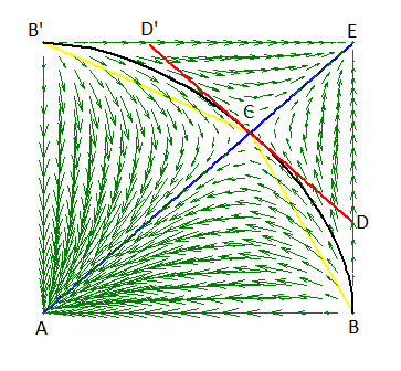
Figure 2: Vector field of replicator dynamics in Stag Hunt.

The Stag Hunt game (figures 1(a)) has two pure Nash, $(Stag,Stag)$ and $(Hare,Hare)$ and a symmetric mixed Nash equilibrium where each agent chooses strategy $Hare$ with probability $2/3$. Stag Hunt replicator trajectories are equivalent those of a coordination game with $w=2$. Coordination games are potential games where the potential function in each state is equal to the utility of each agent. Since the mixed Nash is not weakly stable replicator dynamics converges to pure Nash equilibria for all but a zero measure of initial conditions (Theorem 4.5). When we study the replicator dynamic here, it suffices to examine its projection in the subspace $p_{1s}\times p_{2s}\subset(0,1)^{2}$ which captures the evolution of the probability that each agent assigns to strategy $Stag$ (see figure 2). Using the invariant property of lemma 4.8, we compute the size of each region of attraction in this space and thus provide a quantitative analysis of risk dominance in the classic Stag Hunt game.

Theorem 5.1.

The region of attraction of $(Hare,Hare)$ is the subset of $(0,1)^{2}$ that satisfies $p_{2s}<\frac{1}{2}(1-p_{1s}+\sqrt{1+2p_{1s}-3p_{1s}^{2}})$ and has Lebesgue measure $\frac{1}{27}(9+2\sqrt{3}\pi)\approx 0.7364$. The region of attraction of $(Stag,Stag)$ is the subset of $(0,1)^{2}$ that satisfies $p_{2s}>\frac{1}{2}(1-p_{1s}+\sqrt{1+2p_{1s}-3p_{1s}^{2}})$ and has Lebesgue measure $\frac{1}{27}(18-2\sqrt{3}\pi)\approx 0.2636$. The stable manifold of the mixed Nash equilibrium satisfies the equation $p_{2s}=\frac{1}{2}(1-p_{1s}+\sqrt{1+2p_{1s}-3p_{1s}^{2}})$ and has zero Lebesgue measure.

Proof.

In the case of Stag Hunt games, one can verify in a straightforward manner (via substitution) that $\frac{d\big{(}\frac{2}{3}\ln(\phi_{1s}(t,\mathbf{p}))+\frac{1}{3}\ln(\phi_{1h}(t,\mathbf{p}))-\frac{2}{3}\ln(\phi_{2s}(t,\mathbf{p}))-\frac{1}{3}\ln(\phi_{2h}(t,\mathbf{p}))\big{)}}{dt}=0$, where $\phi_{i\gamma}(t,\mathbf{p})$, corresponds to the probability that each agent $i$ assigns to strategy $\gamma$ at time $t$ given initial condition $\mathbf{p}$. This is a special case of corollary 4.9. We use this invariant function to identify the stable and unstable manifold of the interior Nash $\mathbf{q}$.

Given any point $\mathbf{p}$ of the stable manifold of $\mathbf{q}$, we have that by definition $\lim_{t\rightarrow\infty}\phi(t,\mathbf{p})=\mathbf{q}$. Similarly for the unstable manifold, we have that $\lim_{t\rightarrow-\infty}\phi(t,\mathbf{p})=\mathbf{q}$. The time-invariant property implies that for all such points (belonging to the stable or unstable manifold), $\frac{2}{3}\ln(p_{1s})+\frac{1}{3}\ln(1-p_{1s})$$-\frac{2}{3}\ln(p_{2s})-\frac{1}{3}\ln(1-p_{2s})=\frac{2}{3}\ln(q_{1h})+\frac{1}{3}\ln(1-q_{1h})$$-\frac{2}{3}\ln(q_{2h})-\frac{1}{3}\ln(1-q_{2h})=0$, since the fully mixed Nash equilibrium is symmetric. This condition is equivalent to $p^{2}_{1s}(1-p_{1s})=p^{2}_{2s}(1-p_{2s})$, where $0<p_{1s},p_{2s}<1$. It is straightforward to verify that this algebraic equation is satisfied by the following two distinct solutions, the diagonal line $(p_{2s}=p_{1s})$ and $p_{2s}=\frac{1}{2}(1-p_{1s}+\sqrt{1+2p_{1s}-3p_{1s}^{2}})$. Below, we show that these manifolds correspond indeed to the state and unstable manifold of the mixed Nash, by showing that this Nash equilibrium satisfies these equations and by establishing that the vector field is tangent everywhere along them.

The case of the diagonal is trivial and follows from the symmetric nature of the game. We verify the claims about $p_{2s}=\frac{1}{2}(1-p_{1s}+\sqrt{1+2p_{1s}-3p_{1s}^{2}})$. Indeed, the mixed equilibrium point in which $p_{1s}=p_{2s}=2/3$ satisfies the above equation. We establish that the vector filed is tangent to this manifold by showing in Lemma 8.1 that $\frac{\partial p_{2s}}{\partial p_{1s}}=\frac{\frac{dp_{2s}}{dt}}{\frac{dp_{1s}}{dt}}\mathrel{\hbox to0.0pt{\raisebox{1.29167pt}{$\cdot$}\hss}\raisebox{-1.29167pt}{$\cdot$}}=\frac{p_{2s}\big{(}u_{2}(s)-(p_{2s}u_{2}(s)+(1-p_{2s})u_{2}(h))\big{)}}{p_{1s}\big{(}u_{1}(s)-(p_{1s}u_{1}(s)+(1-p_{1s})u_{1}(h))\big{)}}$, where the last equality is derived by the definition of replicator dynamics. Finally, this manifold is indeed attracting to the equilibrium. Since the function $p_{2s}=y(p_{1s})=\frac{1}{2}(1-p_{1s}+\sqrt{1+2p_{1s}-3p_{1s}^{2}})$ is a strictly decreasing function of $p_{1s}$ in [0,1] and satisfies $y(2/3)=2/3$, this implies that its graph is contained in the subspace $\big{(}0<p_{1s}<2/3\cap 2/3<p_{2s}<1\big{)}\cup\big{(}2/3<p_{1s}<1\cap 0<p_{2s}<2/3\big{)}$. In each of these subsets $\big{(}0<p_{1s}<2/3\cap 2/3<p_{2s}<1\big{)},\big{(}2/3<p_{1s}<1\cap 0<p_{2s}<2/3\big{)}$ the replicator vector field coordinates have fixed signs that “push” $p_{1s},p_{2s}$ towards their respective mixed equilibrium values.

The stable manifold partitions the set $0<p_{1s},p_{2s}<1$ into two subsets, each of which is flow invariant since the unstable manifold itself is flow invariant. Our convergence analysis for the generalized replicator flow implies that in each subset all but a measure zero of initial conditions must converge to its respective pure equilibrium. The size of the lower region of attraction is equal to the following definite integral $\int_{0}^{1}\frac{1}{2}(1-p_{1s}+\sqrt{1+2p_{1s}-3p_{1s}^{2}})dx=\Big{[}1/2\Big{(}p_{1s}-\frac{p_{1s}^{2}}{2}+(-\frac{1}{6}+\frac{p_{1s}}{2})\sqrt{1+2p_{1s}-3p_{1s}^{2}}-\frac{2arcsin[\frac{1}{2}(1-3p_{1s})]}{3\sqrt{3}}\Big{)}\Big{]}_{0}^{1}=\frac{1}{27}(9+2\sqrt{3}\pi)=0.7364$ and the theorem follows. ∎

5.2 Average Price of Anarchy Analysis in Coordination/Consensus Games via Polytope Approximations of Regions of Attraction

We focus on a parametric family of coordination games, as described in figure 1(b). We denote an instance of such a game a $w$-coordination/consensus game. We take the $w$ parameter to be greater or equal to $1$. This game captures strategic situations where agents must learn to coordinate on a single action and where one pure equilibrium (consensus outcome) is preferable for both agents. The initial condition of the replicator dynamics captures each agent’s initial bias. Both agents update their beliefs/distributions by applying the replicator and eventually the system converges to an equilibrium. Interestingly, since the mixed Nash is not weakly stable, Theorem 4.5 implies that the agents will reach a consensus with probability $1$ as long as the initial conditions are chosen according to an arbitrary distribution $F$ admitting a density w.r.t. the Lebesgue measure. A natural such prior (distribution) is the uniform one, since it encodes a total ignorance of the agents’ initial biases. We wish to understand what is the expected system performance given a uniformly random initial condition. Although the inefficient equilibrium will arise with positive probability hopefully its probability is small enough that no matter the $w$ efficiency gap between the two pure equilibria the average system system performance is always within an absolute constant of the optimal, independent of $w$. We will show that this is indeed the case.

Theorem 5.2.

The average price of anarchy of a $w$-coordination game with $w\geq 1$ is at most $\frac{w^{2}+w}{w^{2}+1}$ and at least $\frac{w(w+1)^{2}}{w(w+1)^{2}-2w+2}$.

Sketch. For $w$-coordination games it is straightforward to see that $p^{w}_{1s}(1-p_{1s})-p^{w}_{2s}(1-p_{2s})$ is an invariant property of the replicator system (follows from lemma 4.8). The presence of the parameter $w$ on the exponent precludes the existence of a simple, explicit, parametric description of all the solutions. We analyze the topology of the basins of attractions and produce simple subsets/supersets polytope approximations of them (see figure 2). The volume of these polytope approximations can be computed explicitly and these measures can be used to provide upper and lower bounds on the average case system performance and average price of anarchy. We present the complete proof in the appendix 8.2. ∎

By combining the exact analysis of the standard Stag Hunt game (theorem 5.1), theorem 5.2 and optimizing over $w$ we derive that:

Corollary 5.3.

The average price of anarchy of the class of $w$-coordination games with $w>0$ is at least $\frac{2}{1+\frac{9+2\sqrt{3}\pi}{27}}\approx 1.15$ and at most $\frac{4+3\sqrt{2}}{4+2\sqrt{2}}\approx 1.21$. In comparison, the price of anarchy for this class of games is unbounded.

5.3 Coordination/Consensus Games on a Star Graph

In this subsection we show how to estimate the topology of regions of attraction for star networks of $w$-coordination games. This corresponds to strategic settings where some agents again need to reach consensus but where there is an agent who works as a center communicating with all agents at once. The price of anarchy and stability of these games remain unchanged as we increase the size of the star. Specifically the price of stability is equal to $1$ whereas the price of anarchy can become arbitrarily large for large enough $w$. We will argue once again that the average performance is approximately optimal.

This game has two pure Nash equilibria where all agents either play the first strategy (i.e., $Stag$), or the second (i.e., $Hare$). For simplicity in notation sometimes we denote the first strategy, i.e., $Stag$, as strategy $A$ and the other strategy, i.e., $Hare$, as strategy $B$. This game has a continuum of mixed Nash equilibria. Our goal is to produce an oracle which given as input an initial condition outputs the resulting equilibrium that system converges to.

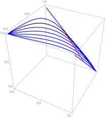
((a)) Examples of stable manifolds for different mixed Nash.

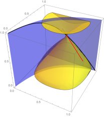
((b)) Stable manifolds lie on the intersection of level sets of invariant functions.

Figure 3: Star network coordination game with $3$ agents

Example. In order to gain some intuition on the construction of these oracles let’s focus on the minimal case with a continuum of equilibria ($N=3$ agents/vertices, center agent with $n=2$ neighbors). Since each agent has two strategies it suffices to depict for each one the probability with which they choose strategy $A$ (the “bad" $Stag$ strategy). Hence, the phase space can be depicted in $3$ dimensions. Figure 3 depicts this phase space. The point $(0,0,0)$ captures the good pure Nash (all $B$), whereas the point $(1,1,1)$ the bad pure Nash (all $A$). There is also a continuum of unstable mixed Nash equilibria. Specifically, it suffices that the center player chooses $A$ with probability $w/(w+1)$ and the summation of the probabilities that the two other agents assign to $A$ is exactly $2w/(w+1)$. In figure 3, we have chosen $w=2$. The continuum of equilibria corresponds to the red straight line. These are unstable equilibria and by Theorem 4.5 almost all initial conditions are attracted to the two attracting pure Nash. For any mixed Nash equilibrium there exists a curve (co-dimension 2) of points that converge to it. Figure 3(a) depicts several such stable manifolds for sample mixed equilibria along the equilibrium line. The union of these stable manifolds partitions the state space into two regions, one attracting to equilibrium $(A,A,A)$ and the other attracting to the equilibrium $(B,B,B)$). Hence, in order to construct our oracle it suffices to have a description of these attracting curves for the mixed equilibria. However, as shown in figure 3(b), we have identified two distinct invariant functions for the replicator dynamic in this system. Given any mixed Nash equilibrium, the set of points of the state space which agree with the value of each of these invariant functions define a set of co-dimension one (the double hollow cone and the curved plane). Any points that converge to this equilibrium must lie on the intersection of these sets (black curve). In fact, due to our point-wise convergence theorem, it immediately follows that this intersection is exactly the stable manifold of the unstable equilibrium. The case for general $N(=n+1)$ works analogously, but now we need to identify $N-1$ ($=n$, equal to the number of neighbors) invariant functions in an algorithmic, efficient manner.

Oracle 1. Input: Initial condition $(x_{1}(0),\dots,x_{n}(0),y(0))$ 2. Output: A or B or mixed 3. If $\sum x_{i}(0)>(\geq)\frac{w}{w+1}n$ and $y(0)\geq(>)\frac{w}{w+1}$ return A. 4. If $\sum x_{i}(0)<(\leq)\frac{w}{w+1}n$ and $y(0)\leq(<)\frac{w}{w+1}$ return B. 5. Compute by solving system 8-9 $x_{1},\dots,x_{n}$ (binary search) 6. Let $f(\rho)=\left(\frac{\rho(w+1)}{w}\right)^{\frac{w}{w+1}}\left[(1-\rho)(w+1)\right]^{\frac{1}{w+1}}-\prod_{i}\left(\frac{x_{i}(0)}{x_{i}}\right)^{x_{i}}\left(\frac{1-x_{i}(0)}{1-x_{i}}\right)^{1-x_{i}}$ 7. if ($\sum_{i}x_{i}(0)>\frac{w}{w+1}n$ and $f(y(0))<0$) or
($\sum_{i}x_{i}(0)<\frac{w}{w+1}n$ and $f(y(0))>0$) return B. 8. if ($\sum_{i}x_{i}(0)>\frac{w}{w+1}n$ and $f(y(0))>0$) or
($\sum_{i}x_{i}(0)<\frac{w}{w+1}n$ and $f(y(0))<0$) return A. 9. return mixed fixed point $(x_{1},\dots,x_{n},\frac{w}{w+1})$

The proof of correctness of the algorithm is presented in Appendix 8.3. Given this oracle, we establish an upper bound of $1.42$ for the average price of anarchy, which is independent both of $w$ as well as the size of the star.

Corollary 5.4.

The average price of anarchy for the class of star $w$-coordination games (with $n+1$ agents) is at most $1.42$.

5.4 Average price of anarchy of linear, symmetric load balancing games

In this subsection, we state the following bounds on the average price of anarchy of linear, symmetric load balancing games.

Theorem 5.5.

The average price of anarchy in terms of makespan of symmetric, linear load balancing games is at most $3/2$. Moreover, generically, the average price of anarchy of symmetric, linear load balancing games is $1$. Specifically, given any number of agents and machines, the set of linear latency functions such that the average price of anarchy of the resulting game is greater than $1$ is a zero measure set within the set of all linear latency functions.

For the classic game of $N$-balls $N$-bins we can show the following theorem:

Theorem 5.6.

The average price of anarchy in terms of makespan for the (identical) $N$-balls $N$-bins is $1$.

6 Conclusion and Open questions

We define an average case analysis notion in dynamical systems focusing on games and replicator dynamics. We call this notion average price of anarchy (APoA) and provide upper and lower bounds for APoA in different classes of games. Several questions arise:

• Other settings/games/mechanisms. In recent followup work, [35] applies our approach to peer prediction mechanisms where the size of the basin of attraction of the truthful equilibrium is used as a proxy for the robustness of truthful play. The replicator model predicts/confirms the significant improvement in robustness of recent mechanisms over earlier approaches. It would be interesting to test the robustness of other (approximately) truthful, differentially private mechanisms in a similar manner.

• Other dynamics. Perform average case analysis for other dynamics and compare them against replicator dynamics.

• Generalization of APoA. Generalize the notion of APoA to dynamics that do not necessarily converge. In particular, it would be intriguing to define an APoA notion for chain recurrent sets (see [29]).

• Point-wise convergence. Generalize the point-wise convergence result to a larger class of congestion games, (e.g., for polynomial cost functions), as well as extend the point-wise convergence result for linear cost functions to other dynamics.

• Volumes of regions of attraction as a function. Given a prior distribution over initial conditions (e.g., uniform), every point-wise convergent dynamical system induces a probability distribution over fixed points. By approximating this function (from priors over initial conditions to posteriors over equilibria), we can predict the average case (long-term) behavior of the system (without having the equations of the dynamics). This interpretation of a game, as an experiment/measurement that maps the outside observer’s original beliefs over initial mixed strategies/beliefs of the agents to (sampling from) a distribution/belief over the resulting equilibria, resolves the non-determinism problem linked to the multiplicity equilibria in a game. The unique, well-defined, deterministic prediction is the function from distributions over initial conditions to distributions over equilibria. Naturally, if the initial distribution is concentrated on a single equilibrium then the output of the prediction function will similarly be concentrated on that equilibrium. Nontrivial distributions will result to a (unique) distribution/prediction that puts positive measure on several equilibria. Developing a formal theory for approximating such functions seems like a fertile ground for combining ideas from computer science and game theory.

APPENDIX

7 Missing proofs and lemmas from Sections 3 and 4

Lemma 7.1.

$\psi(\mathbf{x})$ is a measurable function.

Proof.

For an arbitrary $c\in\mathbb{R}$ we have that

$$\{\mathbf{x}:\psi(\mathbf{x})_{i}<c\}=\cup_{k=1}^{\infty}\cup_{m=1}^{\infty}\cap_{n>m}^{\infty}\{\mathbf{x}:\phi_{n}(\mathbf{x})_{i}<c-\frac{1}{k}\}\}.$$

The set $\{\mathbf{x}:\phi_{n}(\mathbf{x})_{i}<c-\frac{1}{k}\}$ is measurable since $\phi_{n}(\mathbf{x})_{i}$ is a (Lebesgue) measurable function (by continuity). Therefore $\psi(\mathbf{x})_{i}$ is a measurable function. ∎

7.1 Proof of Theorem 4.1 for network coordination games

Proof.

We denote by $\hat{u}_{i}$ the expected utility of agent $i$ under mixed strategy profile $\mathbf{p}$ and by $u_{i\gamma}$ his expected utility when he deviates to strategy $\gamma$ and all other agents still play according to $\mathbf{p}$. We observe that

$$\Psi(\mathbf{p}) =\sum_{i}\hat{u}_{i}=\sum_{i,\gamma}p_{i\gamma}\sum_{j\in N(i)}\sum_{\delta}A_{ij}^{\gamma\delta}p_{j\delta}$$

is a Lyapunov function for our game since (strictly increasing along the trajectories)

$$\frac{\partial\Psi}{\partial p_{i\gamma}} =u_{i\gamma}+\sum_{j\in N(i)}\sum_{\delta}A_{ji}^{\delta\gamma}p_{j\delta}=2u_{i\gamma}\;\textrm{ since }A_{ij}=A_{ji}^{T}$$

and hence

$$\frac{d\Psi}{dt} =\sum_{i,\gamma}\frac{\partial\Psi}{\partial p_{i\gamma}}\frac{dp_{i\gamma}}{dt}=\sum_{i,\gamma,\gamma^{\prime}}p_{i\gamma}p_{i\gamma^{\prime}}(u_{i\gamma}-u_{i\gamma^{\prime}})^{2}\geq 0$$

with equality at fixed points. Hence (as in [17]) we have convergence to equilibrium sets (compact connected sets consisting entirely of fixed points). We address the fact that this doesn’t suffice for pointwise convergence. To be exact it suffices only in the case the equilibria are isolated (which is not the case for network coordination games - see figure 3).

Let $\mathbf{q}$ be a limit point of the trajectory $\mathbf{p}(t)$. W.l.o.g we can assume that $\mathbf{p}(0)$ is in the interior of $\Delta$ and hence $\mathbf{p}(t)$ is in the interior of $\Delta$ for all $t\in\mathbb{R}$ (we can assume that we start in the interior of $\Delta$ otherwise we can just consider the subgame defined by the strategies that agents play with positive probability.). We have that $\Psi(\mathbf{q})\geq\Psi(\mathbf{p}(t))$ where the equality holds only if we start at equilibrium. We define the relative entropy.

$$I(\mathbf{p})=-\sum_{i}\sum_{\gamma:q_{i\gamma}>0}q_{i\gamma}\ln(p_{i\gamma}/q_{i\gamma})\geq 0\textrm{ (Jensen's inequality)}$$

and $I(\mathbf{p})=0$ iff $\mathbf{p}=\mathbf{q}$. We get that

$$\frac{dI}{dt} =-\sum_{i}\sum_{\gamma:q_{i\gamma}>0}q_{i\gamma}(u_{i\gamma}-\hat{u}_{i})$$

$$=\sum_{i}\hat{u}_{i}-\sum_{i,\gamma}q_{i\gamma}u_{i\gamma}$$

$$=\sum_{i}\hat{u}_{i}-\sum_{i,\gamma}\sum_{j\in N(i)}\sum_{\delta}A_{ij}^{\gamma\delta}p_{j\delta}q_{i\gamma}$$

$$=\sum_{i}\hat{u}_{i}-\sum_{j,\delta}\sum_{i\in N(j)}\sum_{\gamma}A_{ij}^{\gamma\delta}p_{j\delta}q_{i\gamma}\;\textrm{ (since }A_{ij}=A_{ji}^{T})$$

$$=\sum_{i}\hat{u}_{i}-\sum_{j,\delta}p_{j\delta}d_{j\delta}$$

$$=\sum_{i}\hat{u}_{i}-\sum_{i}\hat{d}_{i}-\sum_{j,\delta}p_{j\delta}(d_{j\delta}-\hat{d}_{j})$$

$$=\Psi(\mathbf{p})-\Psi(\mathbf{q})-\sum_{i,\gamma}p_{i\gamma}(d_{i\gamma}-\hat{d}_{i})$$

where $d_{i\gamma},\hat{d}_{i}$ correspond to the payoff of agent $i$ if he chooses strategy $\gamma$ and his expected payoff respectively at point $\mathbf{q}$. The rest of the proof follows in a similar way to Losert and Akin [20].

We break the term $\sum_{i,\gamma}p_{i\gamma}(d_{i\gamma}-\hat{d}_{i})$ to positive and negative terms (we ignore zero terms), i.e., $\sum_{i,\gamma}p_{i\gamma}(d_{i\gamma}-\hat{d}_{i})=\sum_{i,\gamma:\hat{d}_{i}>d_{i\gamma}}p_{i\gamma}(d_{i\gamma}-\hat{d}_{i})+\sum_{i,\gamma:\hat{d}_{i}<d_{i\gamma}}p_{i\gamma}(d_{i\gamma}-\hat{d}_{i})$.

Claim: There exists an $\epsilon>0$ so that the function $Z(\mathbf{p})=I(\mathbf{p})+2\sum_{i,\gamma:\hat{d}_{i}>d_{i\gamma}}p_{i,\gamma}$ has $\frac{dZ}{dt}<0$ for $\left\|\mathbf{p}-\mathbf{q}\right\|_{1}<\epsilon$ and $\Psi(\mathbf{q})>\Psi(\mathbf{p})$.

Assuming that $\mathbf{p}\to\mathbf{q}$, we get $u_{i\gamma}-\hat{u}_{i}\to d_{i\gamma}-\hat{d}_{i}$ for all $i,\gamma$. Hence for small enough $\epsilon>0$ with $\left\|\mathbf{p}-\mathbf{q}\right\|_{1}<\epsilon$, we have that $u_{i\gamma}-\hat{u}_{i}\leq\frac{3}{4}(d_{i\gamma}-\hat{d}_{i})$ for the terms which $d_{i\gamma}-\hat{d}_{i}<0$. Therefore

$$\frac{dZ}{dt} =\Psi(\mathbf{p})-\Psi(\mathbf{q})-\sum_{i,\gamma:\hat{d}_{i}<d_{i\gamma}}p_{i\gamma}(d_{i\gamma}-\hat{d}_{i})-\sum_{i,\gamma:\hat{d}_{i}>d_{i\gamma}}p_{i\gamma}(d_{i\gamma}-\hat{d}_{i})+2\sum_{i,\gamma:\hat{d}_{i}>d_{i\gamma}}p_{i\gamma}(u_{i\gamma}-\hat{u}_{i})$$

$$\leq\Psi(\mathbf{p})-\Psi(\mathbf{q})-\sum_{i,\gamma:\hat{d}_{i}<d_{i\gamma}}p_{i\gamma}(d_{i\gamma}-\hat{d}_{i})-\sum_{i,\gamma:\hat{d}_{i}>d_{i\gamma}}p_{i\gamma}(d_{i\gamma}-\hat{d}_{i})+3/2\sum_{i,\gamma:\hat{d}_{i}>d_{i\gamma}}p_{i\gamma}(d_{i\gamma}-\hat{d}_{i})$$

$$=\underbrace{\Psi(\mathbf{p})-\Psi(\mathbf{q})}_{<0}+\underbrace{\sum_{i,\gamma:\hat{d}_{i}<d_{i\gamma}}-p_{i\gamma}(d_{i\gamma}-\hat{d}_{i})}_{\leq 0}+1/2\underbrace{\sum_{i,\gamma:\hat{d}_{i}>d_{i\gamma}}p_{i\gamma}(d_{i\gamma}-\hat{d}_{i})}_{\leq 0}<0$$

where we substitute $\frac{p_{i\gamma}}{dt}=p_{i\gamma}(u_{i\gamma}-\hat{u}_{i})$ (replicator), and the claim is proved.

Note that $Z(\mathbf{p})\geq 0$ (sum of nonnegative terms and $I(\mathbf{p})\geq 0$) and is zero iff $\mathbf{p}=\mathbf{q}.\;$ (i)

To finish the proof of the theorem, if $\mathbf{q}$ is a limit point of $\mathbf{p}(t)$, there exists an increasing sequence of times $t_{n}$, with $t_{n}\to\infty$ and $\mathbf{p}(t_{n})\to\mathbf{q}$. We consider $\epsilon^{\prime}$ such that the set $C=\{\mathbf{p}:Z(\mathbf{p})<\epsilon^{\prime}\}$ is inside $B=\left\|\mathbf{p}-\mathbf{q}\right\|_{1}<\epsilon$ where $\epsilon$ is from claim above. Since $\mathbf{p}(t_{n})\to\mathbf{q}$, consider a time $t_{N}$ where $\mathbf{p}(t_{N})$ is inside $C$. From claim above we get that $Z(\mathbf{p})$ is decreasing inside $B$ (and hence inside $C$), thus $Z(\mathbf{p}(t))\leq Z(\mathbf{p}(t_{N}))<\epsilon^{\prime}$ for all $t\geq t_{N}$, hence the orbit will remain in $C$. By the fact that $Z(\mathbf{p}(t))$ is decreasing in $C$ (claim above) and also $Z(\mathbf{p}(t_{n}))\to Z(\mathbf{q})=0$ it follows that $Z(\mathbf{p}(t))\to 0$ as $t\to\infty$. Hence $\mathbf{p}(t)\to\mathbf{q}$ as $t\to\infty$ using (i). ∎

7.2 Proof of Theorem 4.5

To prove the theorem we will use the Center-Stable Manifold theorem (see Theorem 7.2). In order to do that we need a map whose domain is full-dimensional. However, a simplex in $\mathbb{R}^{n}$ has dimension $n-1$. Therefore, we need to take a projection of the domain space and accordingly redefine the map of the dynamical system. We note that the projection we take will be fixed point dependent; this is to keep the proof that every stable fixed point is a weakly stable Nash proved in [17] relatively less involved later. Let $\mathbf{q}$ be a point of our state space $\Delta$ and $\Sigma=|\cup_{i}S_{i}|$. Let $h_{\mathbf{q}}:[N]\to[\Sigma]$ be a function such that $h_{\mathbf{q}}(i)=\gamma$ if $q_{i\gamma}>0$ for some $\gamma\in S_{i}$. Let $M=\sum|S_{i}|$ and $g$ a fixed projection where you exclude the first coordinate of every agent’s distribution vector. We consider the mapping $z_{\mathbf{q}}:R^{M}\to R^{M-N}$ so that we exclude from each agent $i$ the variable $p_{i,h_{\mathbf{q}}(i)}$ ($z_{\mathbf{q}}$ plays the same role as $g$ but we drop variables with a specific property this time, those played with positive probability). We substitute the variables $p_{i,h_{\mathbf{q}}(i)}$ with $1-\sum_{\gamma\in S_{i}\atop\gamma\neq h_{\mathbf{q}}(i)}p_{i\gamma}$.

The formal statement of the Center-Stable manifold theorem has as follows:

Theorem 7.2.

(Center and Stable Manifolds, p. 65 of [36]) Let $\mathbf{0}$ be a fixed point for the $C^{r}$ local differomorphism $f:U\to\mathbb{R}^{n}$ where $U\subset\mathbb{R}^{n}$ is a neighborhood of zero in $\mathbb{R}^{n}$ and $r\geq 1$. Let $E^{s}\oplus E^{c}\oplus E^{u}$ be the invariant splitting of $\mathbb{R}^{n}$ into generalized eigenspaces of $Df(\mathbf{0})$ corresponding to eigenvalues of absolute value less than one, equal to one, and greater than one. To the $Df(\mathbf{0})$ invariant subspace $E^{s}\oplus E^{c}$ there is associated a local $f$ invariant $C^{r}$ embedded disc $W^{sc}_{loc}$ tangent to the linear subspace at $\mathbf{0}$ and a ball $B$ around zero such that:

$$f(W^{sc}_{loc})\cap B\subset W^{sc}_{loc}.\textrm{ If }f^{n}(\mathbf{x})\in B\textrm{ for all }n\geq 0,\textrm{ then }\mathbf{x}\in W^{sc}_{loc}$$ (4)

For $t=1$ and an unstable fixed point $\mathbf{p}$ we consider the function $\psi_{1,\mathbf{p}}(\mathbf{x})=z_{\mathbf{p}}\circ\phi_{1}\circ z_{\mathbf{p}}^{-1}(\mathbf{x})$ which is $C^{1}$ diffeomorphism, where $\phi_{1}$ is the time one map of the flow of the dynamical system in $\Delta$ (we assume we do the renormalization trick described in Section 3.1). Let $B_{z_{\mathbf{p}}(\mathbf{p})}$ be the ball that is derived from 7.2 and we consider the union of these balls (transformed in $\mathbb{R}^{M}$)

$$A=\cup_{\mathbf{p}}A_{z_{\mathbf{p}}(\mathbf{p})}$$

where $A_{z_{\mathbf{p}}(\mathbf{p})}=g\circ z_{\mathbf{p}}^{-1}(B_{z_{\mathbf{p}}(\mathbf{p})})$ ($z^{-1}_{\mathbf{p}}$ "returns" the set $B_{z_{\mathbf{p}}(\mathbf{p})}$ back to $\mathbb{R}^{M}$). Taking advantage of separability of $\mathcal{R}^{M}$ we have the following theorem.

Theorem 7.3.

(Lindelőf’s lemma) For every open cover there is a countable subcover.

Therefore we can find a countable subcover for $A=\cup_{\mathbf{p}}A_{z_{\mathbf{p}}(\mathbf{p})}$, i.e., $A=\cup_{m=1}^{\infty}A_{z_{\mathbf{p}_{m}}(\mathbf{p}_{m})}$.

Let $\psi_{n,\mathbf{p}}(\mathbf{x})=z_{\mathbf{p}}\circ\phi_{n}\circ z_{\mathbf{p}}^{-1}(\mathbf{x})$. If a point $\mathbf{x}\in g(\Delta)$ (which corresponds to $g^{-1}(\mathbf{x})$ in our original $\Delta$) has as unstable fixed point as a limit, there must exist a $n_{0}$ and $m$ so that $\psi_{n,\mathbf{p}_{m}}\circ z_{\mathbf{p}_{m}}\circ g^{-1}(\mathbf{x})\in B_{z_{\mathbf{p}_{m}}(\mathbf{p}_{m})}$ for all $n\geq n_{0}$ and therefore again from 7.2 and the fact that $\Delta$ is invariant we get that we get that $\psi_{n_{0},\mathbf{p}_{m}}\circ z_{\mathbf{p}_{m}}\circ g^{-1}(\mathbf{x})\in(W_{loc\;z_{\mathbf{p}_{m}}(\mathbf{p}_{m})}^{sc}\cap z_{\mathbf{p}_{m}}(\Delta))$, hence $\mathbf{x}\in g\circ z^{-1}_{\mathbf{p}_{m}}\circ\psi^{-1}_{n_{0},\mathbf{p}_{m}}(W_{loc\;z_{\mathbf{p}_{m}}(\mathbf{p}_{m})}^{sc}\cap z_{\mathbf{p}_{m}}(\Delta))$.

Hence, the set of points in $g(\Delta)$ whose $\omega$-limit has an unstable equilibrium, is a subset of

$$C=\cup_{m=1}^{\infty}\cup_{n=1}^{\infty}g\circ z^{-1}_{\mathbf{p}_{m}}\circ\psi^{-1}_{n,\mathbf{p}_{m}}(W_{loc\;z_{\mathbf{p}_{m}}(\mathbf{p}_{m})}^{sc}\cap z_{\mathbf{p}_{m}}(\Delta))$$ (5)

Observe that the dimension of $W_{loc\;z_{\mathbf{p}_{m}}(\mathbf{p}_{m})}^{sc}$ is at most $M-N-1$ since we assume that $\mathbf{p}_{m}$ is unstable ($\mathcal{J}_{\mathbf{p}_{m}}$ has an eigenvalue with positive real part) and thus $dimE^{u}\geq 1$, hence the set $(W_{loc\;z_{\mathbf{p}_{m}}(\mathbf{p}_{m})}^{sc}\cap z_{\mathbf{p}_{m}}(\Delta))$ has Lebesgue measure zero in $\mathbb{R}^{M-N}$. Finally since $g\circ z^{-1}_{\mathbf{p}_{m}}\circ\psi^{-1}_{n,\mathbf{p}_{m}}:\mathbb{R}^{M-N}\to\mathbb{R}^{M-N})$ is continuously differentiable in an open neighborhood of $g(\Delta)$, $\psi_{n,\mathbf{p}_{m}}$ is $C^{1}$ and hence locally Lipschitz in that neighborhood (see [30] p.71) and it preserves the null-sets (see Lemma 7.4). Namely, $C$ is a countable union of measure zero sets, i.e., is measure zero as well. Since the dynamical system after renormalization is topologically equivalent with the system before renormalization, Theorem 4.5 follows.

Lemma 7.4.

Let $g:\mathbb{R}^{n}\to\mathbb{R}^{n}$ be a locally Lipschitz function, then $g$ is null-set preserving, i.e., for $E\subset\mathbb{R}^{n}$ if $E$ has measure zero then $g(E)$ has also measure zero.

Proof.

Let $B_{\gamma}$ be an open ball such that $\left\|g(\mathbf{y})-g(\mathbf{x})\right\|_{2}\leq K_{\gamma}\left\|\mathbf{y}-\mathbf{x}\right\|_{2}$ for all $\mathbf{x},\mathbf{y}\in B_{\gamma}$. We consider the union $\cup_{\gamma}B_{\gamma}$ which cover $\mathbb{R}^{n}$ by the assumption that $g$ is locally Lipschitz. By Lindelőf’s lemma we have a countable subcover, i.e., $\cup_{i=1}^{\infty}B_{i}$. Let $E_{i}=E\cap B_{i}$. We will prove that $g(E_{i})$ has measure zero. Fix an $\epsilon>0$. Since $E_{i}\subset E$, we have that $E_{i}$ has measure zero, hence we can find a countable cover of open balls $C_{1},C_{2},\dots$ for $E_{i}$, namely $E_{i}\subset\cup_{j=1}^{\infty}C_{j}$ so that $C_{j}\subset B_{i}$ for all $j$ and also $\sum_{j=1}^{\infty}\mu(C_{j})<\frac{\epsilon}{K_{i}^{n}}$. Since $E_{i}\subset\cup_{j=1}^{\infty}C_{j}$ we get that $g(E_{i})\subset\cup_{j=1}^{\infty}g(C_{j})$, namely $g(C_{1}),g(C_{2}),\dots$ cover $g(E_{i})$ and also $g(C_{j})\subset g(B_{i})$ for all $j$. Assuming that ball $C_{j}\equiv B(\mathbf{x},r)$ (center $\mathbf{x}$ and radius $r$) then it is clear that $g(C_{j})\subset B(g(\mathbf{x}),K_{i}r)$ ($g$ maps the center $\mathbf{x}$ to $g(\mathbf{x})$ and the radius $r$ to $K_{i}r$ because of Lipschitz assumption). But $\mu(B(g(\mathbf{x}),K_{i}r))=K_{i}^{n}\mu(B(\mathbf{x},r))=K_{i}^{n}\mu(C_{j})$, therefore $\mu(g(C_{j}))\leq K_{i}^{n}\mu(C_{j})$ and so we conclude that

$$\mu(g(E_{i}))\leq\sum_{j=1}^{\infty}\mu(g(C_{j}))\leq K_{i}^{n}\sum_{j=1}^{\infty}\mu(C_{j})<\epsilon$$

Since $\epsilon$ was arbitrary, it follows that $\mu(g(E_{i}))=0$. To finish the proof, observe that $g(E)=\cup_{i=1}^{\infty}g(E_{i})$ and therefore $\mu(g(E))\leq\sum_{i=1}^{\infty}\mu(g(E_{i}))=0$. ∎

7.3 Proof of Lemma 4.8

Proof.

The derivative of $\sum_{i\in V_{left}}\sum_{\gamma\in S_{i}}q_{i\gamma}\cdot\ln(p_{i\gamma})-\sum_{i\in V_{right}}\sum_{\gamma\in S_{i}}q_{i\gamma}\cdot\ln(p_{i\gamma})$ has as follows:

$$\sum_{i\in V_{left}}\sum_{\gamma\in S_{i}}q_{i\gamma}\frac{d\ln(p_{i\gamma})}{dt}-\sum_{i\in V_{right}}\sum_{\gamma\in S_{i}}q_{i\gamma}\frac{d\ln(p_{i\gamma})}{dt}=\sum_{i\in V_{left}}\sum_{\gamma\in S_{i}}q_{i\gamma}\frac{\dot{p}_{i\gamma}}{p_{i\gamma}}-\sum_{i\in V_{right}}\sum_{\gamma\in S_{i}}q_{i\gamma}\frac{\dot{p}_{i\gamma}}{p_{i\gamma}}=$$

$$= \sum_{i\in V_{left}}\sum_{(i,j)\in E}\big{(}\mathbf{q_{i}}^{\mathrm{T}}A_{ij}\mathbf{p_{j}}-\mathbf{p_{i}}^{\mathrm{T}}A_{ij}\mathbf{p_{j}}\big{)}-\sum_{i\in V_{right}}\sum_{(i,j)\in E}\big{(}\mathbf{q_{i}}^{\mathrm{T}}A_{ij}\mathbf{p_{j}}-\mathbf{p_{i}}^{\mathrm{T}}A_{ij}\mathbf{p_{j}}\big{)}=$$

$$= \sum_{i\in V_{left}}\sum_{(i,j)\in E}\big{(}\mathbf{q_{i}}^{\mathrm{T}}-\mathbf{p_{i}}^{\mathrm{T}}\big{)}A_{ij}\mathbf{p_{j}}-\sum_{i\in V_{right}}\sum_{(i,j)\in E}\big{(}\mathbf{q_{i}}^{\mathrm{T}}-\mathbf{p_{i}}^{\mathrm{T}}\big{)}A_{ij}\mathbf{p_{j}}=$$

$$= \sum_{i\in V_{left}}\sum_{(i,j)\in E}\big{(}\mathbf{q_{i}}^{\mathrm{T}}-\mathbf{p_{i}}^{\mathrm{T}}\big{)}A_{ij}(\mathbf{p_{j}}-\mathbf{q_{j}})-\sum_{i\in V_{right}}\sum_{(i,j)\in E}\big{(}\mathbf{q_{i}}^{\mathrm{T}}-\mathbf{p_{i}}^{\mathrm{T}}\big{)}A_{ij}(\mathbf{p_{j}}-\mathbf{q_{j}})=$$

$$= -\sum_{(i,j)\in E,i\in V_{left},j\in V_{right}}\big{[}\big{(}\mathbf{q_{i}}^{\mathrm{T}}-\mathbf{p_{i}}^{\mathrm{T}}\big{)}A_{ij}(\mathbf{q_{j}}-\mathbf{p_{j}})-\big{(}\mathbf{q_{j}}^{\mathrm{T}}-\mathbf{p_{j}}^{\mathrm{T}}\big{)}A_{ji}(\mathbf{q_{i}}-\mathbf{p_{i}})\big{]}=0$$

where the second to last line follows from the fact that $\mathbf{q}=(\mathbf{q}_{1},\dots,\mathbf{q}_{N})$ is a fully mixed Nash equilibrium. The last equality follows from the fact that all edge/games are coordination/partnership games, i.e., $A_{ji}^{\mathrm{T}}=A_{ij}$. ∎

8 Missing proofs and lemmas of section 5

8.1 Missing proof of technical lemma in 5.1

The following technical lemma argues that the vector filed of the replicator dynamic in the Stag Hunt game is tangent to the curve $p_{2s}=\frac{1}{2}(1-p_{1s}+\sqrt{1+2p_{1s}-3p_{1s}^{2}})$.

Lemma 8.1.

For any $0<p_{1s},p_{2s}<1$, with $p_{2s}=\frac{1}{2}(1-p_{1s}+\sqrt{1+2p_{1s}-3p_{1s}^{2}})$ we have that:

$$\frac{\partial p_{2s}}{\partial p_{1s}}=\frac{\frac{dp_{2s}}{dt}}{\frac{dp_{1s}}{dt}}=\frac{p_{2s}\big{(}u_{2}(s)-(p_{2s}u_{2}(s)+(1-p_{2s})u_{2}(h))\big{)}}{p_{1s}\big{(}u_{1}(s)-(p_{1s}u_{1}(s)+(1-p_{1s})u_{1}(h))\big{)}}$$

Proof.

By substitution of the Stag Hunt game utilities, we have that:

$$\frac{\zeta_{2s}}{\zeta_{1s}}=\frac{p_{2s}\big{(}u_{2}(s)-(p_{2s}u_{2}(s)+(1-p_{2s})u_{2}(h))\big{)}}{p_{1s}\big{(}u_{1}(s)-(p_{1s}u_{1}(s)+(1-p_{1s})u_{1}(h))\big{)}}=\frac{p_{2s}(1-p_{2s})(3p_{1s}-2)}{p_{1s}(1-p_{1s})(3p_{2s}-2)}$$ (6)

However, $p_{2s}(1-p_{2s})=\frac{1}{2}p_{1s}(p_{1s}-1+\sqrt{1+2p_{1s}-3p^{2}_{1s}})$. Combining this with (6),

$$\frac{\zeta_{2s}}{\zeta_{1s}}=\frac{1}{2}\frac{(p_{1s}-1+\sqrt{1+2p_{1s}-3p^{2}_{1s}})(3p_{1s}-2)}{(1-p_{1s})(3p_{2s}-2)}=\frac{1}{2}\frac{(\sqrt{1+3p_{1s}}-\sqrt{1-p_{1s}})(3p_{1s}-2)}{\sqrt{1-p_{1s}}\cdot(3p_{2s}-2)}$$ (7)

Similarly, we have that $3p_{2s}-2=\frac{1}{2}\sqrt{1+3p_{1s}}\cdot(3\sqrt{1-p_{1s}}-\sqrt{1+3p_{1s}})$. By multiplying and dividing equation (7) with $(\sqrt{1+3p_{1s}}+3\sqrt{1-p_{1s}})$ we get:

$$\frac{\zeta_{2s}}{\zeta_{1s}} = \frac{1}{2}\frac{(\sqrt{1+3p_{1s}}+3\sqrt{1-p_{1s}})(\sqrt{1+3p_{1s}}-\sqrt{1-p_{1s}})(3p_{1s}-2)}{2\sqrt{1-p_{1s}}\cdot\sqrt{1+3p_{1s}}\cdot(2-3p_{1s})}$$

$$= -\frac{1}{4}\frac{(\sqrt{1+3p_{1s}}+3\sqrt{1-p_{1s}})(\sqrt{1+3p_{1s}}-\sqrt{1-p_{1s}})}{\sqrt{1+2p_{1s}-3p_{1s}^{2}})}$$

$$= \frac{1}{2}\big{(}-1+\frac{1-3p_{1s}}{\sqrt{1+2p_{1s}-3p_{1s}^{2}}}\big{)}=\frac{\partial\Big{(}\frac{1}{2}(1-p_{1s}+\sqrt{1+2p_{1s}-3p_{1s}^{2}})\Big{)}}{\partial p_{1s}}=\frac{\partial p_{2s}}{\partial p_{1s}}.$$

∎

8.2 Proof of Theorem 5.2

For any $w$, a $w$-coordination game is a potential game and therefore it is payoff equivalent to a congestion game. The only two weakly stable equilibria are the pure ones, hence in order to understand the average case system performance it suffices to understand the size of regions of attraction for each of them. As in the case of Stag Hunt game, we focus on the projection of the system to the subspace $(p_{1s},p_{2s})\subset[0,1]^{2}$.

We denote by $\zeta,\psi$, the projected flow and vector field respectively.

Lemma 8.2.

All but a zero measure of initial conditions in the polytope $(P_{Hare})$:

$$p_{2s} \leq -wp_{1s}+w$$

$$p_{2s} \leq -\frac{1}{w}p_{1s}+1$$

$$0 \leq p_{1s},p_{2s}\leq 1$$

converges to the $(Hare,Hare)$ equilibrium. All but a zero measure of initial conditions in the polytope $(P_{Stag})$:

$$p_{2s} \geq -p_{1s}+\frac{2w}{w+1}$$

$$0 \leq p_{1s},p_{2s}\leq 1$$

converges to the $(Stag,Stag)$ equilibrium.

Proof.

First, we will prove the claimed property for polytope $(P_{Stag})$. Since the game is symmetric, the replicator dynamics are similarly symmetric with $p_{2s}=p_{1s}$ axis of symmetry. Therefore it suffices to prove the property for the polytope $P^{\prime}_{Hare}=P_{Hare}\cap\{p_{2s}\leq p_{1s}\}=\{p_{2s}\leq p_{1s}\}\cap\{p_{2s}\leq-wp_{1s}+w\}\cap\{0\leq p_{1s}\leq 1\}\cap\{0\leq p_{2s}\leq 1\}$ We will argue that this polytope is forward flow invariant, i.e., if we start from an initial condition $\mathbf{x}\in P^{\prime}_{Hare}$ $\psi(t,\mathbf{x})\in P^{\prime}_{Hare}$ for all $t>0$. On the $p_{1s},p_{2s}$ subspace $P^{\prime}_{Hare}$ defines a triangle with vertices $A=(0,0)$, $B=(1,0)$ and $C=(\frac{w}{w+1},\frac{w}{w+1})$ (see figure 2). The line segments $AB$, $AC$ are trivially flow invariant. Hence, in order to argue that the $ABC$ triangle is forward flow invariant, it suffices to show that everywhere along the line segment $BC$ the vector field does not point “outwards” of the $ABC$ triangle. Specifically, we need to show that for every point $p$ on the line segment $BC$ (except the Nash equilibrium $C$), $\frac{|\zeta_{1s}(\mathbf{p})|}{|\zeta_{2s}(\mathbf{p})|}\geq\frac{1}{w}$.

$$\frac{|\zeta_{1s}(\mathbf{p})|}{|\zeta_{2s}(\mathbf{p})|} = \frac{p_{1s}|p_{2s}-(p_{1s}p_{2s}+w(1-p_{1s})(1-p_{2s}))|}{p_{2s}|p_{1s}-(p_{1s}p_{2s}+w(1-p_{1s})(1-p_{2s}))|}=\frac{p_{1s}(1-p_{1s})(w-(w+1)p_{2s})}{p_{2s}(1-p_{2s})(-w+(w+1)p_{1s})}$$

However, the points of the line passing through $B,C$ satisfy $p_{2s}=w(1-p_{1s})$.

$$\frac{|\zeta_{1s}(\mathbf{p})|}{|\zeta_{2s}(\mathbf{p})|} = \frac{wp_{1s}(1-p_{1s})(1-(w+1)(1-p_{1s}))}{w(1-p_{1s})(1-w(1-p_{1s}))(-w+(w+1)p_{1s})}$$

$$= \frac{p_{1s}(-w+(w+1)p_{1s})}{(1-w+wp_{1s})(-w+(w+1)p_{1s})}$$

$$= \frac{p_{1s}}{1-w+wp_{1s}}\geq\frac{p_{1s}}{wp_{1s}}=\frac{1}{w}$$

We have established that the $ABC$ triangle is forward flow invariant. Since the $w$-coordination game is a potential game, all but a zero measurable set of initial conditions converge to one of the two pure equilibria. Since $ABC$ is forward invariant, all but a zero measure of initial conditions converge to $(Hare,Hare)$. A symmetric argument holds for the triangle $AB^{\prime}C$ with $B^{\prime}=(0,1)$. The union of $ABC$ and $AB^{\prime}C$ is equal to the polygon $P_{Hare}$, which implies the first part of the lemma.

Next, we will prove the claimed property for polytope $(P_{Stag})$. Again, due to symmetry, it suffices to prove the property for the polytope $P^{\prime}_{Stag}=P_{Stag}\cap\{p_{2s}\leq p_{1s}\}=\{p_{2s}\leq p_{1s}\}\cap\{p_{2s}\geq-p_{1s}+\frac{2w}{w+1}\}\cap\{0\leq p_{1s}\leq 1\}\cap\{0\leq p_{2s}\leq 1\}$ We will argue that this polytope is forward flow invariant. On the $p_{1s},p_{2s}$ subspace $P^{\prime}_{Stag}$ defines a triangle with vertices $D=(1,\frac{w-1}{w+1})$, $E=(1,1)$ and $C=(\frac{w}{w+1},\frac{w}{w+1})$. The line segments $CD$, $DE$ are trivially forward flow invariant. Hence, in order to argue that the $CDE$ triangle is forward flow invariant, it suffices to show that everywhere along the line segment $CD$ the vector field does not point “outwards” of the $CDE$ triangle (see figure 2) . Specifically, we need to show that for every point $p$ on the line segment $CD$ (except the Nash equilibrium $C$), $\frac{|\zeta_{1s}(\mathbf{p})|}{|\zeta_{2s}(\mathbf{p})|}\leq 1$.

$$\frac{|\zeta_{1s}(\mathbf{p})|}{|\zeta_{2s}(\mathbf{p})|} = \frac{p_{1s}|p_{2s}-(p_{1s}p_{2s}+w(1-p_{1s})(1-p_{2s}))|}{p_{2s}|p_{1s}-(p_{1s}p_{2s}+w(1-p_{1s})(1-p_{2s}))|}=\frac{p_{1s}(1-p_{1s})(w-(w+1)p_{2s})}{p_{2s}(1-p_{2s})(-w+(w+1)p_{1s})}$$

However, the points of the line passing through $C,D$ satisfy $p_{2s}=-p_{1s}+\frac{2w}{w+1}$.

$$\frac{|\zeta_{1s}(\mathbf{p})|}{|\zeta_{2s}(\mathbf{p})|} = \frac{p_{1s}(1-p_{1s})(-w+(w+1)p_{1s})}{(-p_{1s}+\frac{2w}{w+1})(-\frac{w-1}{w+1}+p_{1s})(-w+(w+1)p_{1s})}$$

$$= \frac{p_{1s}(1-p_{1s})}{(-p_{1s}+\frac{2w}{w+1})(-\frac{w-1}{w+1}+p_{1s})}=\frac{p_{1s}(1-p_{1s})}{\frac{2(w-1)}{w+1}(-\frac{w}{w+1}+p_{1s})+p_{1s}(1-p_{1s})}\leq 1$$

We have established that the $CDE$ triangle is forward flow invariant. Since the $w$-coordination is a potential game, all but a zero measurable set of initial conditions converge to one of the two pure equilibria. Since $CDE$ is forward invariant, all but a zero measure of initial conditions converge to $(Stag,Stag)$. A symmetric argument holds for the triangle $CD^{\prime}E$ with $D^{\prime}=(\frac{w-1}{w+1},1)$. The union of $CDE$ and $CD^{\prime}E$ is equal to the polygon $P_{Stag}$, which implies the second part of the lemma. ∎

Proof.

The measure/size of $\mu(P_{Hare})=2|ABC|=\frac{w}{w+1}$, and similarly the measure of $\mu(P_{Stag})=2|CDE|=\frac{2}{(w+1)^{2}}$. The average limit performance of the replicator satisfies $\int_{g(\Delta)}sw(\psi(x))d\mu\geq 2w\cdot\mu(P_{Hare})+2\big{(}1-\mu(P_{Hare})\big{)}=2\frac{w^{2}+1}{w+1}$. Furthermore, $\int_{g(\Delta)}sw(\psi(x))d\mu\leq 2w\big{(}1-\mu(P_{Stag})\big{)}+2\cdot\mu(P_{Stag})=2w(1-\frac{2}{(w+1)^{2}})+2\cdot\frac{2}{(w+1)^{2}}=2w-4\frac{w-1}{(w+1)^{2}}$. This implies that $\frac{w(w+1)^{2}}{w(w+1)^{2}-2w+2}\leq APoA\leq\frac{w^{2}+w}{w^{2}+1}$. ∎

8.3 Analysis of N-star graph

Notation. To simplify notation in this section, we rename strategy $Stag$ as strategy $A$ and strategy $Hare$ as strategy $B$. Let’s consider a mixed strategy profile as $(\bf{x_{1}},\dots,\bf{x_{n}},\bf{y})$ where $\bf{x_{i}}$ denotes the mixed strategy of “leaf" agent $i$, and $\bf{y}$ denotes the mixed strategy of the center agent. Since it suffices to track for each agent the probability with which they play strategy $A$, i.e., Hare, we will sometimes abuse notation and denote the mixed strategy of agent $i$ by $x_{i}\mathrel{\hbox to0.0pt{\raisebox{1.29167pt}{$\cdot$}\hss}\raisebox{-1.29167pt}{$\cdot$}}=x_{iA}$, i.e., the probability with which he is playing strategy $A$ as well as denote a mixed strategy profile by $(x_{1},\dots,x_{n},y)$.

“leaf" Here is the high level idea of the analysis: We start by showing that the only fixed points with region of attraction with positive measure are those in which all agents choose strategy $A$ or all agents choose strategy $B$. After that we show that the limit point of any nontrivial trajectory will be either one of the two mentioned, or a mixed Nash. Therefore we need to compute the regions of attraction of the two fixed points where all choose $A$ or all choose $B$. To do that, we need to compute the boundary of these two regions (namely the Center-Stable manifold of the fully mixed ones). This happens as follows: Given an initial point $(x_{1}(0),\dots,x_{n}(0),y(0))$, we compute the possible fully mixed limit point $(x_{1},\dots,x_{n},\frac{w}{w+1})$ (there can only be one such possible limit point due to point-wise convergence which is furthermore constrained due to Lemma 8.3 below) that is on the boundary of the two regions. If the initial condition is on the upper half space w.r.t to the possible fully mixed limit point $(x_{1},\dots,x_{n},\frac{w}{w+1})$ the dynamics converge to the everyone playing $A$, otherwise to everyone playing $B$.

8.3.1 Structure of fixed points

If a “leaf" agent $i$ applies a randomized/mixed strategy at a fixed point, it must be the case that the strategy of the center agent $y=\frac{w}{w+1}$. Otherwise, the “leaf" agent would strictly prefer either strategy $A$ or strategy $B$. Hence the fixed points of the star graph game have the following structure: If the center agent has a pure strategy, then all agents must be pure. If the center agent has a mixed strategy, then $\sum_{i}x_{i}=\frac{w}{w+1}n$. In that case, if all the “leaf" agents have pure strategies then $y$ can have any value in $[0,1]$, otherwise $y=\frac{w}{w+1}$.

8.3.2 Invariants

Lemma 8.3.

$[\ln(x_{i}(t))-\ln(1-x_{i}(t))]-[\ln(x_{j}(t))-\ln(1-x_{j}(t))]$ is invariant for all $i,j$ (independent of $t$).

Proof.

$\frac{d}{dt}[\ln(x_{i}(t))-\ln(1-x_{i}(t))]-\frac{d}{dt}[\ln(x_{j}(t))-\ln(1-x_{j}(t))]=[y-w(1-y)]-[y-w(1-y)]=0.$ ∎

Next, we will argue that if we start in the interior of $\Delta$, the system can converge to fixed points, where either all agent play A or B, or to a fully mixed Nash where $y=\frac{w}{w+1}$ and $\sum x_{i}=\frac{w}{w+1}n$.

Lemma 8.4.

For all initial conditions in the interior of $\Delta$, either the dynamic converges to all A’s, i.e, (1,…,1), or to all B’s, i.e., (0,…, 0), or to some fully mixed fixed point, i.e, $(x_{1},\dots,x_{n},\frac{w}{w+1})$ with $0<x_{i}<1$ for all $i$, and $\sum_{i}x_{i}=\frac{w}{w+1}n$.

Proof.

We consider the following two cases:

• If $x_{i}(t)\to 1$ for some $i$, then $\ln(x_{i}(t))-\ln(1-x_{i}(t))\to+\infty$. So from Lemma 8.3 for every $j$ we get that $\ln(x_{j}(t))-\ln(1-x_{j}(t))\to+\infty$, hence $x_{j}(t)\to 1$. Due the structure of the equilibrium set and pointwise convergence, $y(t)$ must converge to $0$ or $1$. Due the fact that the fixed point $(1,\dots,1,0)$ is repelling we get that the system converges to all A’s. The same argument is used if $x_{i}(t)\to 0$ for some $i$.

• If the dynamic converges to an equilibrium were all “leaf" agents are mixed, then $y=\frac{w}{w+1}$ and $\sum_{i}x_{i}=\frac{w}{w+1}n$ because by the analysis of the structure of the fixed points that is the only possibility.

∎

Let $(x_{1}(0),\dots,x_{n}(0),y(0))$ be the initial condition, where $x_{i}(0),y(0)$ are the probabilities agent $i$, center agent choose $A$ ($1-x_{i}(0),1-y(0)$ will be the probability to choose $B$) respectively. By Lemma 8.4, we know that the corresponding trajectory will converge either to the all A’s equilibrium or the all B’s equilibrium or a fully mixed one. Next, by using Lemma 8.3 we will narrow down the possibilities for this fully mixed equilibrium to a single one, which we denote by $(x_{1},\dots,x_{n},\frac{w}{w+1})$.

For each leaf agent $i>1$, we define a positive constant $c_{i}$ such that

$$c_{i}=\frac{x_{i}(0)/(1-x_{i}(0))}{x_{1}(0)/(1-x_{1}(0))}.$$

Due to Lemma 8.3 the quantity $\frac{x_{i}(t)/(1-x_{i}(t))}{x_{1}(t)/(1-x_{1}(t))}$ is time invariant. Hence, the limit point $(x_{1},\dots,x_{n},\frac{w}{w+1})$ must satisfy this condition, i.e,

$$x_{i} =\frac{c_{i}x_{1}}{1+(c_{i}-1)x_{1}}$$ (8)

Moreover, by Lemma 8.4 it must satisfy $\sum x_{i}=\frac{w}{w+1}n$, which combined with (8) implies that:

$$\sum_{i}\frac{c_{i}x_{1}}{1+(c_{i}-1)x_{1}}=\frac{w}{w+1}n$$ (9)

where we have defined $c_{1}=1$.

Observe that the function $f(x)=\frac{cx}{1+(c-1)x}$ is strictly increasing in $[0,1]$ (given any fixed positive $c$) and $f(0)=0,f(1)=1$. Therefore $g(x)=\sum_{i}\frac{c_{i}x}{1+(c_{i}-1)x}-\frac{w}{w+1}n$ is strictly increasing in $[0,1]$ (as sum of strictly increasing functions in $[0,1]$) and $g(0)=-\frac{w}{w+1}n<0$ and $g(1)=n-\frac{w}{w+1}n>0$. Thus, it has always a unique solution in $[0,1]$ and equivalently the system of equations (8,9) has a unique solution. Together with $y=\frac{w}{w+1}$, the equilibrium limit point lies in the interior of $\Delta$. Given $x_{1}(0),\dots,x_{n}(0)$ we can compute (approximate with arbitrary small error $\epsilon$) $x_{1},\dots,x_{n}$ via binary search (using Bolzano’s theorem).

Lemma 8.5.

Since star graph is a bipartite graph from Lemma 4.8 we have that since $(x_{1},\dots,x_{n},y)$ is a fully mixed Nash then along any system trajectory $((x_{1}(t),\dots,x_{n}(t),y(t)))$ the function

$$\frac{w}{w+1}\ln(y(t))+\frac{1}{w+1}\ln(1-y(t))-\sum_{i}[x_{i}\ln(x_{i}(t))+(1-x_{i})\ln(1-x_{i}(t))]$$

is (time) invariant, i.e. independent of $t$.

Lemma 8.6.

If $y(t)\geq(>)\frac{w}{w+1}$ and $\sum x_{i}(t)>(\geq)\frac{w}{w+1}n$ for some $t$, the trajectory converges to all $A$’s and if $y(t)\leq(<)\frac{w}{w+1}$ and $\sum x_{i}(t)<(\leq)\frac{w}{w+1}n$ for some $t$, the trajectory converges to all $B$’s.

Proof.

In the first case, $y(t)$ is increasing and $x_{i}(t)$ (for all $i$) are non-decreasing and thus $y(t^{\prime})>\frac{w}{w+1}$ and $\sum x_{i}(t^{\prime})>\frac{w}{w+1}n$ holds for all $t^{\prime}>t$. In the second case $y(t)$ is decreasing and $x_{i}(t)$ (for all $i$) are non-increasing and thus $y(t^{\prime})<\frac{w}{w+1}$ and $\sum x_{i}(t^{\prime})<\frac{w}{w+1}n$ holds for all for $t^{\prime}>t$. Combining this with Lemma 8.4, concludes the proof when we consider the first combination of inequalities. The second combination of inequalities follows in a similar manner. ∎

Therefore if a trajectory converges to the fully mixed equilibrium $(x_{1},\dots,x_{n},\frac{w}{w+1})$ then at any time $t$ we must have $\sum x_{i}(t)>\frac{w}{w+1}n$ and $y(t)<\frac{w}{w+1}$ ($x_{1}(t),\dots,x_{n}(t)$ are decreasing and $y(t)$ increasing) or $\sum x_{i}(t)<\frac{w}{w+1}n$ and $y(t)>\frac{w}{w+1}$ ($x_{1}(t),\dots,x_{n}(t)$ are increasing and $y(t)$ decreasing). Combining all the facts together, we get that the stable manifold of the fixed point $(x_{1},\dots,x_{n},\frac{w}{w+1})$ can be described as follows: $(x_{1}(0),\dots,x_{n}(0),y(0))$ lies on the stable manifold if $\sum_{i}x_{i}(0)>n\frac{w}{w+1}$ and $y(0)<\frac{w}{w+1}$ or $\sum_{i}x_{i}(0)<n\frac{w}{w+1}$ and $y(0)>\frac{w}{w+1}$ and by Lemma 8.5 we get that

$$y(0)^{\frac{w}{w+1}}(1-y(0))^{\frac{1}{w+1}}=c\prod_{i}x_{i}(0)^{x_{i}}(1-x_{i}(0))^{1-x_{i}},$$ (10)

where $c=\frac{\left(\frac{w}{w+1}\right)^{\frac{w}{w+1}}\left(\frac{1}{w+1}\right)^{\frac{1}{w+1}}}{\prod_{i}(x_{i})^{x_{i}}(1-x_{i})^{1-x_{i}}}$.

Lemma 8.7.

The function $x^{w}(1-x)$ is strictly increasing in $[0,\frac{w}{w+1}]$ and decreasing in $[\frac{w}{w+1},1]$.

By Lemma 8.7 we have that there exist at most two $y(0)$ that satisfy (10), one which is $\geq\frac{w}{w+1}$ and one that $\leq\frac{w}{w+1}$. If $\sum x_{i}(0)<n\frac{w}{w+1}$, $y(0)$ should be the largest root of the two so that dynamics converges to the fully mixed, otherwise the smallest root. If now the initial condition $y(0)$ does not satisfy (10), then the dynamics converges to all $A$’s if $y(0)$ is greater that it is supposed (so that dynamics converges to the fully mixed) and to all $B$’s otherwise. Therefore we have the oracle below:

8.3.3 Oracle Algorithm

Oracle 1. Input: Initial condition $(x_{1}(0),\dots,x_{n}(0),y(0))$ 2. Output: A or B or mixed 3. If $\sum x_{i}(0)>(\geq)\frac{w}{w+1}n$ and $y(0)\geq(>)\frac{w}{w+1}$ return A. 4. If $\sum x_{i}(0)<(\leq)\frac{w}{w+1}n$ and $y(0)\leq(<)\frac{w}{w+1}$ return B. 5. Compute by solving system 8-9 $x_{1},\dots,x_{n}$ (binary search) 6. Let $f(\rho)=\left(\frac{\rho(w+1)}{w}\right)^{\frac{w}{w+1}}\left[(1-\rho)(w+1)\right]^{\frac{1}{w+1}}-\prod_{i}\left(\frac{x_{i}(0)}{x_{i}}\right)^{x_{i}}\left(\frac{1-x_{i}(0)}{1-x_{i}}\right)^{1-x_{i}}$ 7. if ($\sum_{i}x_{i}(0)>\frac{w}{w+1}n$ and $f(y(0))<0$) or
($\sum_{i}x_{i}(0)<\frac{w}{w+1}n$ and $f(y(0))>0$) return B. 8. if ($\sum_{i}x_{i}(0)>\frac{w}{w+1}n$ and $f(y(0))>0$) or
($\sum_{i}x_{i}(0)<\frac{w}{w+1}n$ and $f(y(0))<0$) return A. 9. return mixed fixed point $(x_{1},\dots,x_{n},\frac{w}{w+1})$

Remark: Given any point from $\Delta$ uniformly at random, under the assumption of solving exactly the equations to compute $x_{1},\dots,x_{n}$ to arbitrary high precision the probability that the oracle above returns mixed is zero.

8.4 Proof of Corollary 5.4

Proof.

We first prove the following claim.

Claim 8.8.

$\mathbb{P}\left[\sum x_{i}(0)\leq n\frac{w}{w+1}\right]$ is increasing with $n$.

Proof.

We set by $X_{1},...,X_{n}$ the random starting points $x_{i}(0),...,x_{n}(0)$. Let $S_{n}:=\sum_{i=1}^{n}X_{i}$, $x\in\mathbb{R}$, $n=2,3,\dots$, and

$$G_{n}(x):=P(S_{n}/n\leq x)=\frac{1}{n!}\,\sum_{j}(-1)^{j}\binom{n}{j}(nx-j)_{+}^{n},$$

where $u_{+}:=\max(0,u)$; (Irwin–Hall distribution). We may assume that the summation above is over all integers $j$, where $\binom{n}{j}=0$ if $j\notin\{0,\dots,n\}$. Let

$$D_{n}(x):=G_{n+1}(x)-G_{n}(x).$$ (11)

It suffices to show that $D_{n}(\frac{w}{w+1})\geq 0$ for $w\geq 1$.

First observe that $D_{n}$ is $n-1$ times continuously differentiable, $D_{n}=0$ outside $(0,1)$, and also holds that $D_{n}(1-x)=-D_{n}(x)$ (by symmetry). For small $x>0$ we get $G_{n}(x)=\frac{1}{n!}\,n^{n}x^{n}>\frac{1}{(n+1)!}\,(n+1)^{n+1}x^{n+1}=G_{n+1}(x)$, whence $D_{n}(x)<0$, whence $D_{n}>0$ in a left neighborhood of $1$, with $D_{n}(1)=0$ and $D_{n}(1/2)=0$. It suffices to show that $D_{n}$ has no roots in $(1/2,1)$ since $1>\frac{w}{w+1}\geq 1/2$.

Suppose the contrary. By the symmetry, $D_{n}$ has at least $3$ roots in $(0,1)$. Then, by Rolle theorem, the derivative $G_{n}^{(n-1)}$ of $G_{n}$ of order $n-1$ has at least $3+n-1=n+2$ roots in $(0,1)$. This contradicts the fact (we prove below) that, for each integer $j$ such that $n-1\geq j\geq\frac{n-1}{2}$, $D_{n}$ has exactly one root in interval

$$h_{n,j}:=[\tfrac{j}{n},\tfrac{j+1}{n}).$$

Indeed, take any $x\in[1/2,1]$. It is not hard to see that, for $j_{x}:=j_{n,x}:=\lfloor nx\rfloor$,

$$G_{n}^{(n-1)}(x)=n^{n-1}\sum_{j=0}^{j_{x}}(-1)^{j}\binom{n}{j}(nx-j)$$

$$=\frac{n^{n-1}}{n-1}(-1)^{j_{x}}\binom{n}{j_{x}+1}({j_{x}}+1)((n-1)x-{j_{x}}).$$

Similarly, for $k_{x}:=j_{n+1,x}$,

$$G_{n+1}^{(n-1)}(x)=\frac{(n+1)^{n-1}}{2n(n-1)}(-1)^{k_{x}}\binom{n+1}{k_{x}+1}(k_{x}+1)P(n,k_{x},x),$$

where

$$P(n,k,x):=-2k\left(n^{2}-1\right)x+k(kn-1)+n\left(n^{2}-1\right)x^{2}.$$

Note that $k_{x}\in\{j_{x},j_{x}+1\}$. We consider the following two cases.

Case 1: $k_{x}=j_{x}=j\in[\frac{n-1}{2},n-1]$, which is equivalent to $x\in h^{\prime}_{n,j}:=[\frac{j}{n},\frac{j+1}{n+1})$. It also follows that in this case $j\geq n/2$. In this case, it is not hard to check that $D_{n}(x)$ equals $(-1)^{j}P_{n,j,1}(x)$ in sign, where

$$P_{n,j,1}(x):= 2jn^{n}(n-j)+x\left(-2(n-1)n^{n}(n-j)-2j(n+1)^{n}\left(n^{2}-1\right)\right)+$$

$$j(n+1)^{n}(jn-1)+(n+1)^{n}\left(n^{2}-1\right)nx^{2},$$

which is convex in $x$. Moreover, $P_{n,j,1}(\frac{j}{n})$ and $P_{n,j,1}(\frac{j+1}{n+1})$ each equals $2n^{n}-(1+n)^{n}<0$ in sign. So, $P_{n,j,1}<0$ and hence $D_{n}$ has no roots in $h^{\prime\prime}_{n,j}=[\frac{j}{n},\frac{j+1}{n+1})$.

Case 2: $k_{x}=j+1$ and $j_{x}=j\in[\frac{n-1}{2},n-1]$, which is equivalent to $x\in h^{\prime\prime}_{n,j}:=[\frac{j+1}{n+1},\frac{j+1}{n})$. In this case, it is true that $D_{n}(x)$ equals $(-1)^{j+1}P_{n,j,2}(x)$ in sign, where

$$P_{n,j,2}(x):= (j+1)\left((n+1)^{n}(jn+n-1)-2jn^{n}\right)+2(j+1)\left((n-1)n^{n}-(n+1)^{n}\left(n^{2}-1\right)\right)x+$$

$$n\left(n^{2}-1\right)(n+1)^{n}x^{2},$$

and is convex in $x$. Moreover, $P_{n,j,1}(\frac{j+1}{n})$ and $-P_{n,j,1}(\frac{j+1}{n+1})$ equal $2n^{n}-(1+n)^{n}<0$ in sign. So, $P_{n,j,2}$ has exactly one root in $h^{\prime\prime}_{n,j}$ and hence so does $D_{n}$.

Since the interval $h_{n,j}$ is the disjoint union of $h^{\prime}_{n,j}$ and $h^{\prime\prime}_{n,j}$, $D_{n}$ has exactly one root in $h_{n,j}=[\tfrac{j}{n},\tfrac{j+1}{n})$, and the proof is complete. ∎

There are exactly two possible outcomes with positive probability; all the agents choose strategy $A$ and all choose strategy $B$. Assume we take one sample at random $(x_{1},\dots,x_{n},y)$ from $\times_{i=1}^{n+1}\Delta_{2}$ where $n+1$ are the number of agents. Let $p_{x},p_{y}$ be the the probability that a sample at random satisfies $\sum_{i}x_{i}\leq n\frac{w}{w+1}$ and $y<\frac{w}{w+1}$ respectively. It turns out from the oracle above on the star-graph game (see also discussion earlier) that if ($\sum_{i}x_{i}<n\frac{w}{w+1}$ and $y<\frac{w}{w+1}$) or ($\sum_{i}x_{i}<n\frac{w}{w+1}$ and $f(y)>0$) or ($\sum_{i}x_{i}>n\frac{w}{w+1}$ and $f(y)<0$) then the dynamics eventually converges to all agents choose $B$. Hence the region of attraction of the outcome all agents choose $B$ will be at least the probability $p_{x}\cdot p_{y}\geq\frac{w}{w+1}\cdot\frac{w}{w+1}$ (by Claim 8.8 for $n=1$ is minimum). Since the optimal is $w(n+1)$, we get that the average price of anarchy is at most $\frac{w(n+1)}{(\frac{w}{w+1})^{2}w(n+1)+(1-(\frac{w}{w+1})^{2})(n+1)}=\frac{w(w+1)^{2}}{w^{3}+2w+1}$. The quantity $\frac{w(w+1)^{2}}{w^{3}+2w+1}$ is less than $1.42$. ∎

8.5 Proof of Theorem 5.5

In this section, we will prove the following bounds on the average price of anarchy of linear, symmetric load balancing games. We will break down the proof of theorem 5.5 into several technical lemmas. The next definition encodes Nash equilibria where randomizing agents do not “interact” with each other.

Definition 8.9.

We call a mixed Nash equilibrium of a load balancing game to be almost pure, if the intersection of the supports of the strategies of any two randomizing agents contains only edges whose latency functions are constant functions.

Lemma 8.10.

The average price of anarchy of a symmetric, linear load balancing games is at most equal to the ratio of the cost of the worst almost pure Nash equilibrium divided by the cost of the optimal outcome.

Proof.

By corollary 4.6 we have that for all but a zero measure of initial conditions replicator dynamics converges to weakly stable equilibria. By definition, weakly stable equilibria have the property that given any two agents with mixed strategies strategies if one agent deviates to one the strategies in his support and plays it with probability one then the second agent should still stay indifferent between the strategies in his support. If there exists two agents with mixed strategies such that the intersection of their supports contains machines with strictly increasing latency functions then if one agent deviates to playing that machine with probability one, he will strictly increase the cost experienced by the second agent on that machine, whereas by this deviation he can only decrease the cost of all other machines in the support of the second agent. The second agent is no longer indifferent between the strategies in his support and thus the initial equilibrium was not weakly stable. In the worst case average price of anarchy places all of the probability mass of initial conditions to the worst almost pure Nash equilibrium. In this case the average price of anarchy would be equal to the ratio of the cost of the worst almost pure Nash equilibrium divided by the cost of the optimal outcome. ∎

Lemma 8.11.

In symmetric linear load balancing games all pure Nash equilibria have optimal makespan.

Proof.

Suppose not, that is, suppose that there exists a pure Nash equilibrium whose makespan, i.e., the load of the most congested machine, is not optimal amongst all outcomes/configurations. That means that its most loaded machine must be a machine with a strictly increasing cost function that has higher load than its load at the optimal outcome. Hence, there must be another machine whose load is strictly less than its load at the optimal configuration. If we move one agent from the first to the second machine we claim that its cost will strictly decrease. Indeed, its new latency is at most the latency of the second machine in the optimal configuration, which is less or equal to the optimal makespan, which by hypothesis is strictly less than the makespan of the first configuration, which was its original cost. Hence, the original configuration cannot be a Nash equilibrium and we have reached a contradiction. ∎

Lemma 8.12.

In any symmetric, linear load balancing games the ratio of the cost of the worst almost pure Nash equilibrium divided by the cost of the optimal outcome is at most 3/2. Furthermore, this bound is tight.

Proof.

First, we create the lower bound. We have a load balancing game with two agents and three machines. The latency function for the first machine is $3x$ whereas for the other two machines is $2x$. It is straightforward to check that the strategy outcome where the first agent chooses the first machine and the second agent chooses one of the remaining two machines uniformly at random is a Nash equilibrium and, in fact, a weakly stable one. The makespan of this equilibrium is $3$, whereas the optimal state has each of the two agents choosing deterministically one of the last two machines and using it by themselves. The makespan of that outcome is $2$, which results in a lower bound of $3/2$.

Next, we will show that this bound is tight. First, we will establish that it suffices to examine Nash equilibria where the intersection between the supports of the mixed strategies of any two randomizing agents is empty. Indeed, suppose that we have two randomizing agents where the intersection of their supports contains some machines with constant latency functions. If we force one of the two agents to deviate and choose deterministically the strategy of constant latency in his support then the makespan of the state remains constant and furthermore the outcome is still a weakly stable Nash. The reason that it remains a Nash is that if an agent wished to deviate to some strategy used by the deviating agent originally, then when deviating to that machine he would experience exactly the same cost as when using the machine with the constant cost function. Thus, he could have profitably deviated in the initial configuration. This is impossible since that configuration was a Nash equilibrium. Trivially, this new Nash equilibrium is weakly stable since we have only decreased the number of randomizing agents and the supports of the remaining randomizing agents remained the same. We can keep performing these deviations up until there no longer randomizing agents for which the intersection of the supports contains any machine (of constant latency function). Hence, in terms of identifying the almost pure Nash equilibrium with the worst makespan it suffices to focus on the set of almost mixed Nash equilibria where the intersection of the supports of any two randomizing agents is empty.

We have established that if suffices to focus on mixed Nash equilibria where each machine has at most one randomizing agent. We will establish that the makespan of each such equilibrium is within a $3/2$ factor of the makespan of a pure Nash equilibrum, which by Lemma 8.11 implies that it is within a $3/2$ factor of the optimal makespan. The argument is as follows: We will start from the mixed Nash and will proceed by fixing the randomizing agents to playing strategies in their support with probability one. We start from the randomizing agent $i$ that experiences minimum cost amongst all randomizing agents. We fix him to playing the strategy in his support that he chose with minimal probability in the original mixed Nash. We also fix the rest of the randomizing agents to arbitrary strategies in their support. Next, we repeatedly go through all agents in decreasing cost order and we allow each agent to move and migrate to the least expensive (available) machine if it is strictly cheaper than his current machine. Due to symmetry once we find one agent who does not wish deviate all of the rest of the agents do not wish to deviate either due to symmetry of the available machines. This process will terminate at equilibrium since this is a potential game. Furthermore, agent $i$ (nor of any of the other agents in his machine) will ever move during this process. If he did move then there would exist at some point a profitable deviating move from him. However, immediately after fixing the randomizing agents to choosing something in their current support, agent $i$ did not have any improving deviations since his experienced cost was minimal amongst all randomizing agents and hence at least as small as the cost of any deviation. In fact, the cheapest available deviations are exactly the strategies that belonged in his support. As we allow costly agents to move greedily from their current strategy to the best available strategy the cost of the best available deviation cannot decrease with time. Thus, agent $i$ will not deviate. Hence, the makespan at the resulting pure Nash equilibrium will be at least equal the cost of agent $i$ when his was fixed to the strategy that he played with minimal probability. If we denote that edge as $e$ and its load (excluding agent $i$) as $x_{e}$ then this implies that the makespan at the resulting Nash and thus the optimal makespan is at least $a_{e}(x_{e}+1)+b_{e}$. However, the original mixed state was an equilibrium and if agent $i$ played strategy $e$ with probability $p$ then no agent in the original Nash equilibrum would experience cost more than $a_{e}(x_{e}+p+1)+b_{e}$. But since $e$ was chosen to be the strategy played with minimal probability in his original support $p\leq 1/2$ and hence no agent can experience cost more than $a_{e}(x_{e}+3/2)+b_{e}$. So, the original makespan is at most $a_{e}(x_{e}+3/2)+b_{e}$ and the optimal makespan is at least $a_{e}(x_{e}+1)+b_{e}$. The ratio between these two terms becomes maximal (and equal to $3/2$) for $b_{e}=0$ and $x_{e}=0$, which is exactly satisfied by our tight lower bound. ∎

Remark 8.13.

If we slightly perturb the above tight example so that the latency function for the first machine is $3x$ whereas for the other two machines is $2x+\epsilon$ then the continuum of equilibria with the bad makespan will have a non-negligible region of attraction resulting in an average price of anarchy which is strictly greater than one.

Lemma 8.14.

In generic symmetric linear load balancing games the set of almost pure Nash equilibria coincides with the set of pure Nash equilibria. Specifically, the set of linear latency functions such the set of almost pure Nash equilibria is a strict superset of the set of pure Nash equilibria is of measure zero within the set of all linear latency functions.

Proof.

We will show that if a linear symmetric load balancing game has an almost pure Nash equilibrium that is not pure, i.e., that has at least one agent using a randomized strategy, then the coefficients of the linear latency functions belong to a zero measure set. Indeed, let’s focus on one of the randomizing agents. Since this agent is indifferent between (at least) two machines/edges $e,e^{\prime}$ and he is the only randomizing agent using these machines (or some of these machines have a constant latency function) then there exist integer numbers $k,k^{\prime}$, so that the cost of these two machines are equal under loads $k,k^{\prime}$. This implies that $a_{e}\cdot k+b_{e}=a_{e^{\prime}}\cdot k^{\prime}+b_{e}^{\prime}$. However, for any fixed $k,k^{\prime}$ the set of coefficients $a_{e},a_{e^{\prime}},b_{e},b_{e^{\prime}}$ that satisfy this linear equation is a zero-measure set. Hence, given any number of agents and machines the set of latency functions that have almost pure Nash equilibria that are not pure can be expressed as a countable union of zero-measure sets, which is a zero-measure set. ∎

By combining the lemmas of this section, Theorem 5.5 follows immediately.

8.6 Proof of Theorem 5.6

In the classic game of $N$ identical balls/agents, with $N$ identical bins/machines, each ball chooses a distribution over the bins selfishly and we assume that the cost of bin $\gamma$ is equal to $\gamma$’s load. We know for this game that the PoA is $\Omega(\frac{\log N}{\log\log N})$ [8]. We will prove that the Average PoA is $1$. This is derived via corollary 4.6 and by showing that in this case the set of weakly stable Nash equilibria coincides with the set of pure equilibria.

Lemma 8.15.

In the problem of $N$ identical balls and $N$ identical bins every weakly stable Nash equilibrium is pure.

Proof.

Assume we have a weakly Nash equilibrium $\mathbf{p}$. From corollary 4.6, we have the following facts:

• Fact 1: For every bin $\gamma$, if a agent $i$ chooses $\gamma$ with probability $1>p_{i\gamma}>0$, he must be the only agent that chooses that bin with nonzero probability. Let $i,j$ two agents that choose bin $\gamma$ with nonzero probabilities and also $p_{i\gamma},p_{j\gamma}<1$. Clearly if agent $i$ changes his strategy and chooses bin $\gamma$ with probability one, then agent $j$ doesn’t stay indifferent (his cost $c_{i\gamma}$ increases).

• Fact 2: If agent $i$ chooses bin $\gamma$ with probability one, then he is the only agent that chooses bin $\gamma$ with nonzero probability. This is true because every ball/agent $j\neq i$ can find a bin with load less than 1 to choose.

From Facts 1,2 and since the number of balls is equal to the number of bins we get that $\mathbf{p}$ must be pure. ∎

Proof.

Hence from Lemma  8.15 and 4.6 we get that for all but measure zero starting points of $g(\Delta)$, the replicator converges to pure Nash equilibria. Every pure Nash equilibrium (each ball chooses a distinct bin) has social cost (makespan) $1$, which is the optimal makespan. Hence the Average PoA is $1$. ∎

Remark: The lemma below shows how crucial is Lindelőf’s lemma (essentially separability of $R^{m}$ for all $m$) in the proof of Theorem 4.5. Even simple and well studied instances of games with constant number of agents and strategies may have uncountably many equilibria. In such games, naive union bound arguments do not suffice since we cannot argue about the measure of an uncountable union of measure zero sets.

Lemma 8.16.

Let $n\geq 4$ then the set of Nash equilibria of the $N$ balls $N$ bins game is uncountable.

Proof.

We will prove it for $N=4$ and then the generalization is easy, i.e., if $N>4$ then the first 4 agents will play as shown below in the first 4 bins and each of the remaining $N-4$ agent will choose a distinct remaining bin. Below we give matrix $A$ where $A_{i\gamma}=p_{i\gamma}$. Observe that for any $x\in[\frac{1}{4},\frac{3}{4}]$ we have a Nash equilibrium.

$$A=\left(\begin{array}[]{cccc}x&1-x&0&0\\ 1/2&0&1/2&0\\ 0&1/2&0&1/2\\ 0&0&x&1-x\end{array}\right).$$

∎

References

- [1] H. Ackermann, P. Berenbrink, S. Fischer, and M. Hoefer. Concurrent imitation dynamics in congestion games. In PODC, pages 63–72, 2009.
- [2] A. Asadpour and A. Saberi. On the inefficiency ratio of stable equilibria in congestion games. In WINE, pages 545–552, 2009.
- [3] P. Berenbrink, T. Friedetzky, L. A. Goldberg, P. W. Goldberg, Z. Hu, and R. Martin. Distributed selfish load balancing. SIAM J. Comput., pages 1163–1181, 2007.
- [4] P. Berenbrink, T. Friedetzky, I. Hajirasouliha, and Z. Hu. Convergence to equilibria in distributed, selfish reallocation processes with weighted tasks. Algorithmica, 62(3-4):767–786, 2012.
- [5] Y. Cai and C. Daskalakis. On minmax theorems for multiplayer games. In SODA, pages 217–234, 2011.
- [6] N. Cesa-Bianchi and G. Lugoisi. Prediction, Learning, and Games. Cambridge University Press, 2006.
- [7] C. Chung, K. Ligett, K. Pruhs, and A. Roth. The price of stochastic anarchy. In SAGT, pages 303–314, 2008.
- [8] A. Czumaj and B. Vőcking. Tight bounds for worst-case equilibria. In ACM Trans. Algorithms. ACM, 2007.
- [9] C. Daskalakis and C. H. Papadimitriou. On a network generalization of the minmax theorem. In ICALP, pages 423–434, 2009.
- [10] E. Even-Dar and Y. Mansour. Fast convergence of selfish rerouting. In SODA, pages 772–781, 2005.
- [11] D. Fotakis, A. C. Kaporis, and P. G. Spirakis. Atomic congestion games: Fast, myopic and concurrent. In Algorithmic Game Theory, volume 4997 of Lecture Notes in Computer Science, pages 121–132. 2008.
- [12] D. Fudenberg and D. K. Levine. The Theory of Learning in Games. MIT Press Books. The MIT Press, 1998.
- [13] J. C. Harsanyi and R. Selten. A General Theory of Equilibrium Selection in Games. Cambridge: MIT Press., 1988.
- [14] J. Hofbauer and K. Sigmund. Evolutionary Games and Population Dynamics. Cambridge University Press, Cambridge, 1998.
- [15] H. Khalil. Nonlinear Systems. Prentice Hall, 1996.
- [16] R. Kleinberg, K. Ligett, G. Piliouras, and É. Tardos. Beyond the Nash equilibrium barrier. In ICS, 2011.
- [17] R. Kleinberg, G. Piliouras, and É. Tardos. Multiplicative updates outperform generic no-regret learning in congestion games. In STOC, 2009.
- [18] J. D. Lee, M. Simchowitz, M. I. Jordan, and B. Recht. Gradient descent only converges to minimizers. In COLT, 2016.
- [19] K. Ligett and G. Piliouras. Beating the best Nash without regret. SIGecom Exchanges 10, 2011.
- [20] V. Losert and E. Akin. Dynamics of games and genes: Discrete versus continuous time. Journal of Mathematical Biology, 1983.
- [21] R. Mehta, I. Panageas, and G. Piliouras. Natural selection as an inhibitor of genetic diversity: Multiplicative weights updates algorithm and a conjecture of haploid genetics. In ITCS, 2015.
- [22] R. Mehta, I. Panageas, G. Piliouras, P. Tetali, and V. V. Vazirani. Mutation, Sexual Reproduction and Survival in Dynamic Environments. ArXiv e-prints, 2015.
- [23] R. Mehta, I. Panageas, G. Piliouras, and S. Yazdanbod. The Computational Complexity of Genetic Diversity. ESA, 2016.
- [24] D. Monderer and L. S. Shapley. Potential games. Games and Economic Behavior, pages 124–143, 1996.
- [25] R. B. Myerson. Game Theory: Analysis of Conflict. Harvard University Press., 1991.
- [26] N. Nisan, T. Roughgarden, E. Tardos, and V. V. Vazirani. Algorithmic Game Theory. Cambridge University Press, 2007.
- [27] M. A. Nowak. Evolutionary Dynamics. Harvard University Press, 2006.
- [28] I. Panageas and G. Piliouras. Gradient descent only converges to minimizers: Non-isolated critical points and invariant regions. CoRR, 2016.
- [29] C. H. Papadimitriou and G. Piliouras. From nash equilibria to chain recurrent sets: Solution concepts and topology. In ITCS, pages 227–235, 2016.
- [30] L. Perko. Differential Equations and Dynamical Systems. Springer, 1991.
- [31] G. Piliouras, C. Nieto-Granda, H. I. Christensen, and J. S. Shamma. Persistent patterns: Multi-agent learning beyond equilibrium and utility. In AAMAS, pages 181–188, 2014.
- [32] G. Piliouras and J. S. Shamma. Optimization despite chaos: Convex relaxations to complex limit sets via Poincaré recurrence. In SODA, 2014.
- [33] T. Roughgarden. Intrinsic robustness of the price of anarchy. In STOC, pages 513–522, 2009.
- [34] W. H. Sandholm. Population Games and Evolutionary Dynamics. MIT Press, 2010.
- [35] V. Shnayder, R. Frongillo, and D. C. Parkes. Measuring Performance Of Peer Prediction Mechanisms Using Replicator Dynamics. In IJCAI, 2016.
- [36] M. Shub. Global Stability of Dynamical Systems. Springer-Verlag, 1987.
- [37] H. P. Young. Strategic Learning and its Limits. Oxford University Press, 2004.
- [38] B. Zhang and J. Hofbauer. Equilibrium selection via replicator dynamics in 2x2 coordination games. International Journal of Game Theory, 44(2):433–448, 2014.