Discovery of a rich proto-cluster at $z=2.9$ and associated diffuse cold gas in the VIMOS Ultra-Deep Survey (VUDS)

High-density environments are crucial places for studying the link between hierarchical structure formation and stellar mass growth in galaxies. In this work, we characterise a massive proto-cluster at $z=2.895$ that we found in the COSMOS field using the spectroscopic sample of the VIMOS Ultra-Deep Survey (VUDS). This is one of the rare structures at $z\sim 3$ not identified around an active galactic nucleus (AGN) or a radio galaxy, thus it represents an ideal laboratory for investigating the formation of galaxies in dense environments. The structure comprises 12 galaxies with secure spectroscopic redshift in an area of $\sim 7^{\prime}\times 8^{\prime}$, in a total $z$ range of $\Delta z=0.016$. The measured galaxy number overdensity is $\delta_{g}=12\pm 2$. This overdensity has a total mass of $M\sim 8.1\times 10^{14}M_{\odot}$ in a volume of $13\times 15\times 17$ Mpc³. Simulations indicate that such an overdensity at $z\sim 2.9$ is a proto-cluster, which will collapse in a cluster of total mass $M_{z=0}\sim 2.5\times 10^{15}M_{\odot}$ at $z=0$, i.e. a massive cluster in the local Universe. We analysed the properties of the galaxies within the overdensity, and we compared them with a control sample at the same redshift but outside the overdensity. We could not find any statistically significant difference between the properties (stellar mass, star formation rate, specific star formation rate, NUV-r and r-K colours) of the galaxies inside and outside the overdensity, but this result might be due to the lack of statistics or possibly to the specific galaxy population sampled by VUDS, which could be less affected by environment than the other populations not probed by the survey. The stacked spectrum of galaxies in the background of the overdensity shows a significant absorption feature at the wavelength of Ly$\alpha$ redshifted at $z=2.895$ ($\lambda=4736$Å), with a rest frame equivalent width ($EW$) of $4\pm 1.4$Å. Stacking only background galaxies without intervening sources at $z\sim 2.9$ along their line of sight, we find that this absorption feature has a rest frame EW of $10.8\pm 3.7$Å, with a detection S/N of $\sim 4$. We verify that this measurement is not likely to be due to noise fluctuations. These EW values imply a high column density (N(HI)$\sim 3-20\times 10^{19}$cm^-2), consistent with a scenario where such absorption is due to intervening cold streams of gas that are falling into the halo potential wells of the proto-cluster galaxies. Nevertheless, we cannot rule out the hypothesis that this absorption line is related to the diffuse gas within the overdensity.

1 Introduction

The detection and study of (proto) clusters at high redshift is important input for cosmological models, and these high-density environments are crucial places for studying the link between hierarchical structure formation and stellar mass growth in galaxies at early times. The earlier the epoch when an overdensity is detected, the more powerful the constraints on models of galaxy formation and evolution because of the shorter cosmic time over which physical processes have been able to work. Specifically, in high-redshift ($z\gtrsim 1.5-2$) (proto) clusters the study of how environment affects the formation and evolution of galaxies is particularly effective, because galaxies had their peak of star formation at such redshifts (Madau et al. 1996; Cucciati et al. 2012).

However, the sample of high-redshift ($z\gtrsim 1.5$) structures detected so far is still limited, and it is very heterogeneous, spanning from relaxed to unrelaxed systems. Many detection techniques have been used that are based on different (and sometimes apparently contradicting) assumptions. For instance, the evolution of galaxies in clusters appears to be accelerated relative to low-density regions (e.g. Steidel et al. 2005). As a result, while the average SFR of a galaxy decreases with increasing local galaxy density in the low-redshift Universe, this trend should reverse at earlier times, with the SFR increasing with increasing galaxy density (Cucciati et al. 2006; Elbaz et al. 2007). Indeed, some (proto-) clusters have been identified at high redshift as overdensities of star-forming galaxies (Capak et al. 2011), such as Ly$\alpha$ emitters (Steidel et al. 2000; Ouchi et al. 2003, 2005; Lemaux et al. 2009) and H$\alpha$ emitters (Hatch et al. 2011). At the same time, in some high-$z$ overdensities an excess of massive red galaxies has also been observed (e.g. Kodama et al. 2007; Spitler et al. 2012), and other dense structures have been identified via a red-sequence method (e.g. Andreon et al. 2009) or via an excess of IR luminous galaxies (e.g. Gobat et al. 2011; Stanford et al. 2012) or LBGs (e.g. Toshikawa et al. 2012).

High-$z$ overdensities have also been identified by using other observational signatures, for instance with the Sunyaev-Zeldovich effect (Sunyaev & Zeldovich 1972, 1980) as in Foley et al. (2011), or searching for diffuse X-ray emission (e.g. Fassbender et al. 2011), or looking for photometric redshift overdensities in deep multi-band surveys (Castellano et al. 2007; Salimbeni et al. 2009; Scoville et al. 2013; Chiang et al. 2014). Moreover, assuming a synchronised growth of galaxies with that of their super-massive black holes, high-redshift proto-structures have been searched for around AGNs (e.g. Miley et al. 2004) and radio galaxies (e.g. Pentericci et al. 2000; Matsuda et al. 2009; Galametz et al. 2012), even if an excess of galaxies around high-$z$ QSOs has not always been found (see e.g. Decarli et al. 2012). However, this approach could introduce unknown selection effects, for example those due to the influence of powerful radio galaxies on the surrounding environment. The study of proto-structures selected only on the basis of the redshift distribution of its members is more likely to offer an unbiased view of high-density environments at high redshift and allow a comparison with the habitat of radio galaxies and quasars. Nevertheless, it is necessary to obtain spectroscopic redshifts of member galaxies, which is a costly observational task at high redshifts. Spectroscopic surveys conducted with visible wavelength spectrographs will observe the UV rest frame light of galaxies at redshifts $z>2$, and therefore be mostly sensitive to star-forming galaxies.

Although the sample of (proto) clusters at $z>1.5$ is increasing in number, it is a heterogeneous data set. This inhomogeneity prevents using it to assess the abundance of clusters at such redshifts, which could be used to constrain cosmological parameters (e.g. Borgani et al. 1999; Ettori et al. 2009). Chiang et al. (2013) have recently made an attempt to find a common parameter to group and analyse the known overdensities at high $z$. They used simulations to study the probability of given overdensities at $z=2-5$ to collapse in bound clusters at $z=0$, and, in case of collapse, the mass at $z=0$ ($M_{z=0}$) of such clusters. They also give prescriptions for computing $M_{z=0}$ using the overdensity of the proto-cluster within a given volume. Following their own prescriptions, in a second work (Chiang et al. 2014) they perform a homogeneous search for overdensities using the photometric redshifts in the COSMOS field. We come back to their analysis in the following sections.

The discovery and study of an overdensity at high $z$ also naturally addresses how a dense environment affects galaxy formation and evolution. Galaxies can build their stellar masses via abrupt processes like mergers, which in some cases produce an increase in mass up to a factor of two or so, or via more continuous processes based on in-situ star formation. At the same time, other physical processes are likely at work to quench star formation (such as AGN and SNe feedback), and some of these processes are particularly effective in high-density environments, where the gas reservoirs in galaxies can be stripped during interactions with the intra-cluster medium (ICM).

The relative role of all these processes as a function of cosmic time is still a matter of debate. In recent years, many observational studies have focused on analysing the merger rate. If at $z<1$ the evolution of merger rate is quite well constrained for both major and minor mergers (i.e. with a luminosity/mass ratio greater or less than $\sim 1/4$, see e.g. de Ravel et al. 2009 and López-Sanjuan et al. 2011), at $z>1$ observational results still show a large scatter (see e.g. López-Sanjuan et al. 2013 and Tasca et al. 2014 for the most recent studies). On the side of stellar mass growth via smooth star formation, some theoretical models support a scenario where massive ($M_{baryon}\sim 10^{11}M_{\odot}$ ) galaxies at $z\sim 2-3$ are efficiently fed by narrow, cold (e.g. $T\sim 10^{4}$ K), intense, partly clumpy, gaseous streams that penetrate the shock-heated halo gas into the inner galaxy with rates of the order of 100 $M_{\odot}{\rm yr}^{-1}$ . These streams can grow a dense, unstable, turbulent disc with a bulge and trigger rapid star formation (e.g. Kereš et al. 2005; Dekel et al. 2009). Observational evidence of gas accretion is still limited (Giavalisco et al. 2011; Bouché et al. 2013), and further studies are needed to support this scenario. Simulations (Kimm et al. 2011) show that the covering fraction of dense cold gas is larger in more massive haloes, suggesting that the best environment for testing the cold flow accretion scenario are high-redshift over-dense regions.

In this paper, we present the discovery of an overdensity at $z\sim 2.9$ in the COSMOS field, detected in the deep spectroscopic survey VUDS (VIMOS Ultra-Deep Survey). In Sect. 2 we describe our data. In Sect. 3 we describe the overdensity and compute the total mass that it comprises, and also its possible evolution to $z=0$. Section 4 shows the search for diffuse cold gas in the overdensity, as inferred by absorption lines in the spectra of background galaxies. In Sect. 5 we analyse the properties of the galaxies in the overdensity and contrast them to a sample of galaxies outside the structure at a similar redshift. Finally, in Sect. 6 we discuss our results and summarise them in Sect.7.

We adopt a flat $\Lambda$CDM cosmology with $\Omega_{m}=0.27$, $\Omega_{\Lambda}=0.73$, and $H_{0}=70$ km s^-1 Mpc^-1. Magnitudes are expressed in the AB system.

2 Data

The VUDS survey is fully described in Le Fevre et al. (2014), so we give only a brief summary here. VUDS is a spectroscopic survey using VIMOS on the ESO-VLT (Le Fèvre et al. 2003), targeting mainly $z>2$ galaxies in one square degree in three fields: COSMOS, ECDFS, and VVDS-2h. Spectroscopic targets have been mainly selected based on a photometric redshift ($z_{p}$) cut. Photometric redshifts are derived with the code Le Phare (Arnouts et al. 1999; Ilbert et al. 2006) using the multi-wavelength photometry available in the survey fields, and they have an accuracy of $\sigma_{zp}\simeq 0.04(1+z)$ for magnitudes $i_{AB}\leq 25$ in the COSMOS field (see Ilbert et al. 2013). The primary criterion for target selection in VUDS is for targets to satisfy $z_{p}+1\sigma_{zp}>2.4$ and $i_{AB}\leq 25$. To account for degeneracies in the $z_{p}$ computation, in this criterion $z_{p}$ could be either the first or second peak of the $z_{p}$ probability distribution function.

The VIMOS spectra have been observed with 14h integrations with the LRBLUE (R=230) and LRRED (R=230) grisms, covering a combined wavelength range 3600 $<\lambda<9350\AA$. This integration time allows reaching S/N $\sim 5$ on the continuum (at $\lambda\sim 8500$Å) for galaxies with $i_{AB}=25$, and S/N $\sim 5$ for an emission line with a flux $F=1.5\times 10^{-18}erg/s/cm^{2}/\AA$.

The spectroscopic redshift accuracy with this setup is $\sigma_{zs}=0.0005(1+z)$ (Le Fèvre et al. 2013), corresponding to $\sim 150\,{\rm km\,s}^{-1}$. Data reduction, redshift measurement, and assessment of the reliability of measured redshift are described in full detail in Le Fevre et al. (2014). In brief, data are reduced within the VIPGI environment (Scodeggio et al. 2005), and then the spectroscopic redshifts are measured with the software EZ (Garilli et al. 2010). EZ is based on the cross-correlation with templates. We used templates derived from previous VIMOS observations of the VVDS and zCOSMOS surveys. A first redshift measurement is obtained by a blind EZ run, then two different team members inspect the result, separately, and modify it if needed. Finally, the two measurements are compared and the two measurers provide, in agreement, a single final measurement.

During the measurement process, a reliability flag is also assigned to each measured redshift by the two measurers, namely flag=1, 2, 3, 4, 9. Based on previous VIMOS surveys similar to VUDS (see e.g. the VVDS survey, Le Fèvre et al. 2013), the redshifts with flag=1, 2, 3, 4, 9 should have a probability of being right of $\sim 50,80,98,100,80$%, respectively. The precise assessment of such probability values for VUDS is ongoing. There are also objects with flag=0, i.e. when no redshift could be assigned. Brighter than $i_{AB}=25$, the fraction of VUDS targets with a reliable redshift measurement (i.e. flag=2,3,4,9) is $\sim 74$%.

2.1 Ancillary photometric data and rest-frame galaxy properties

In addition to the VIMOS spectroscopic data, a large set of imaging data is available in the three fields. In particular, the COSMOS field (Scoville et al. 2007) has a full coverage with the HST-ACS F814W filter (Koekemoer et al. 2007) and includes, among other data, $BVriz$ photometry from Subaru (Capak et al. 2007; Taniguchi et al. 2007), and the more recent $YJHK$ photometry from the UltraVista survey (McCracken et al. 2012).

Absolute magnitudes, stellar masses ($\mathcal{M}$), and star formation rates (SFRs) for the spectroscopic sample and for the photometric parent catalogue were computed using the code Le Phare as described in Ilbert et al. (2013), using the measured spectroscopic redshift when available. The method is based on a spectral energy distribution (SED) fitting technique. We used a template set that comprises Bruzual & Charlot (2003) templates. We assumed the Calzetti et al. (2000) extinction law and included emission line contributions as described in Ilbert et al. (2009). We used a library based on a composite of delayed star formation histories (SFH) and exponentially declining SFHs, with nine possible $\tau$ values ranging from 0.1 Gyr to 30 Gyr.

The typical statistical error on $\mathcal{M}$ and SFR is $\sim 0.15$ and $0.18$ dex, respectively, at $z\sim 3$, i.e. the redshift of interest in this work. Moreover, we tested which is the impact of the choice of different SFHs on $\mathcal{M}$ and SFR. We recomputed the SED fitting another two times, in one case using only delayed SFHs and then using only exponentially declining SFHs. We find that the difference on the derived $\mathcal{M}$ among the two SFH sets is negligible, as also found in Ilbert et al. (2013). In contrast, there is a systematic offset of $\sim 0.05$ dex between the SFR based on delayed SFHs and the SFR based on exponentially declining SFHs, with a scatter around the offset of about 0.03 dex.

The absolute magnitude computation is optimised using the full information given by the multi-band photometric data described above. To limit the template dependency, absolute magnitudes in each band are based on the observed magnitude in the band that, redshifted in the observer frame, is the closest to the given absolute magnitude band (see Appendix A.1 in Ilbert et al. 2005). Because of this adopted method, the biggest source of uncertainty on the absolute magnitude computation is the error on the closest observed magnitude, and there is essentially no difference when using different SFHs. Namely, the typical errors on the $NUV$, $r$, and $K$ absolute magnitudes used in this paper (see Sect.5) are of the order of 0.06, 0.1, and 0.15 magnitudes, respectively.

Given the main selection of our sample, i.e. $i_{AB}\leq 25$, VUDS mainly probes (relatively) star-forming galaxies at the redshift of interest for this paper ($z\sim 3$), where the $i$-band corresponds to the rest frame ultra-violet emission. For instance, we verified that our sample, at $z\sim 3$, does not probe in a complete way the range of specific SFR (sSFR) at $\log_{10}(sSFR[yr^{-1}])\lesssim-9$ with respect to a catalogue selected in $K$-band (namely, $K\leq 24$, like the one in Ilbert et al. 2013). Galaxies with such a low sSFR, which are missed by our survey, are generally the most massive ones ($\log_{10}(M/M_{\odot})\gtrsim 10.5$).

Figure 1: Top: right ascension (RA) and declination (Dec) distribution of VUDS galaxies in the COSMOS field (dark dots). Red filled circles: VUDS galaxies within $2.8858\leq z\leq 2.9018$ in the VIMOS quadrant where the structure has been found (P2Q1). Orange open diamonds: other VUDS galaxies within $2.8858\leq z\leq 2.9018$ but outside P2Q1. The blue rectangles show the VIMOS footprint. Bottom: like the top panel, but zoomed-in in the region of P2Q1. Green open circles are VUDS galaxies at $z\geq 3$, and blue open circles are ‘free-line-of-sight’ VUDS galaxies at $z\geq 3$ (see text for details).

Figure 2: VUDS redshift distribution in the COSMOS field (black) and in the quadrant of the structure (red), in redshift bins of $\Delta z=0.01$.

3 The spectroscopic overdensity

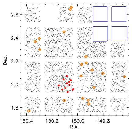
Using the VUDS spectroscopic data, we discovered a galaxy overdensity in the COSMOS field at $z=2.895$. It comprises 12 galaxies with reliable spectroscopic redshifts (1 galaxy with flag=2, 11 galaxies with flag 3 or 4) in a very narrow redshift bin ($\Delta z=0.016$, namely $2.8858\leq z\leq 2.9018$) in a region covered by a single VIMOS quadrant. The distribution in right ascension (RA) and declination (Dec) of the VUDS galaxies in the COSMOS field and, in particular, of those at $2.8858\leq z\leq 2.9018$ is shown in the top panel of Fig. 1. The panel also shows the VIMOS typical footprint, made by four quadrants. Namely, 11 out of 12 galaxies have been detected in quadrant Q1 of the pointing F51P002 (P2Q1 from now on), and 1 in the adjacent quadrant F51P005 Q4 (same $RA$ as P2Q1 but at higher $Dec$). The two quadrants overlap, so this twelfth galaxy is within the area covered by P2Q1. From now on, we consider this galaxy as part of P2Q1. One VIMOS quadrant covers a region of $\sim 7^{\prime}\times 8^{\prime}$, which corresponds, at $z\sim 2.9$, to $\sim 13\times 15$ Mpc² comoving, or $\sim 3.4\times 3.9$ Mpc² physical.

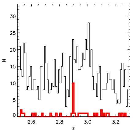
Figure 2 shows the VUDS redshift distribution in the COSMOS field and the one in P2Q1, both made using only reliable redshifts (flag=2, 3, 4, and 9), in redshift bins of $\Delta z=0.01$. There is an evident peak of ten galaxies in P2Q1 at $z=2.895$, with two other galaxies in the two adjacent redshift bins, for a total of 12 galaxies in $\Delta z=0.016$. In all the quadrants in the three VUDS fields, in the range $2.5<z<3.3$, the median number of spectroscopic galaxies with reliable redshifts falling in such narrow $z$ bins is 0. In only 1.5% of the cases these narrow bins comprise more than three galaxies, and always less than seven, with the exception of the structure described in this paper. The few cases with 5-6 spectroscopic galaxies within $\Delta z=0.016$ will be inspected in detail in a future work. Using the 12 galaxies in the overdensity, we measured a velocity dispersion along the line of sight of $\sigma_{los}=299\pm 70\,{\rm km\,s}^{-1}$, but we cannot assume that the galaxy velocities in our overdensity follow a Gaussian distribution. A more appropriate estimator of the dispersion of a non-Gaussian (or contaminated Gaussian) distribution is the “biweight method”, which has been proven to also be very robust in case of small number statistics (see case C in Beers et al. 1990, and references therein). With this method we estimate $\sigma_{los}=270\pm 80\,{\rm km\,s}^{-1}$. We retain this second estimation as the velocity dispersion of the galaxies in the overdensity.

We notice that we did not find any broad line AGN among the 12 VUDS galaxies. In the Chandra-COSMOS (Elvis et al. 2009) and XMM-COSMOS (Cappelluti et al. 2007) catalogues, it has not been detected any extended nor point-like source that matches the galaxies in the structure (Cappelluti, private communication), and we found only one match with the sources in the Herschel PEP (Lutz et al. 2011) catalogue.

We also explored whether the overdensity discovered in the VUDS spectroscopy survey is detectable using photometric redshifts, i.e. in the $RA$-$Dec$-$z_{p}$ space. To do this, we applied both the Voronoi Tessellation algorithm (Voronoi 1908) and the DEDICA algorithm (Bardelli et al. 1998). The two methods give equivalent results, so we discuss only the DEDICA results. DEDICA is an algorithm based on an adaptive kernel method estimate of the density field, also estimating the significance of the detected structures. We used the VUDS photometric parent catalogues, with the most recent photometric redshifts obtained by also using the YJHK bands of the UltraVista survey. To maximise the signal, we limited the analysis of the photometric redshift catalogue to the $i$-band range $[24-25]$ (the same range that comprises the 12 spectroscopic galaxies in the overdensity) and to the redshift range $[2.72-3.19]$. The choice of this redshift range is due to the mean difference between the photometric ($z_{p}$) and spectroscopic redshift ($z_{s}$) of the 12 galaxies in the overdensity. We found $\langle z_{p}-z_{s}\rangle=0.06\pm 0.12$. To choose the redshift range for the photometric redshifts, first we applied this shift of 0.06 to the redshift of the structure, then we considered a range of $\pm 1\sigma=\pm 0.12$ around this redshift. After running the algorithm on this photometric data set, we found no significant overdensities (at $90\%$) in the region of our structure. We obtained the same result by increasing the photometric redshift range up to $\pm 2\sigma$ and also without applying the shift.

We verified with a simple model whether our spectroscopic overdensity, given its characteristics, would be detectable in the parent photometric catalogue using photometric redshifts as described above. We assumed a sampling rate of $\sim 25$% in P2Q1 for the spectroscopic galaxies in the $i$-band range $[24-25]$ (see the following section). This would give us $\sim 50$ galaxy members in the overdensity in the full parent photometric catalogue. We modelled the $z_{s}$ of these 50 galaxies to be distributed with $\sigma_{los}=270\pm 80\,{\rm km\,s}^{-1}$, centred on $z=2.895$. To this $z_{s}$ distribution, we added a random photometric error extracted from a Gaussian distribution with $\sigma=0.12$ (found above). We repeated this computation 1000 times, and each time we counted the number of galaxies within the redshift range $[2.72-3.19]$, and computed the overdensity $\delta_{g}$ with respect to all the galaxies in the photometric catalogue in the same redshift range (and with $i$-band magnitude in the range $[24-25]$). We found $\delta_{g}=0.62\pm 0.1$, i.e. $\sim 20$ times lower than the value we find using spectroscopic redshift (see next section).

We conclude that, given the characteristics of the spectroscopic overdensity (number of member galaxies and measured velocity dispersion), it is unlikely to detect it using photometric redshifts with a typical error like the ones we used. In the recent works by Scoville et al. (2013) and Chiang et al. (2014), who identify overdensities in the COSMOS field using photometric redshifts, no overdensity at the position of P2Q1 at $z\sim 2.9$ is detected, but they both find a very close overdensity at about the same redshift. Namely, Chiang et al. (2014) have published a list of proto-cluster candidates in the COSMOS field (see their Table 1). Among these candidates, the closest in the $RA-Dec$ plane to our proto-cluster has ID=30, with $RA=150.009$ and $Dec=1.974$, so very close ($\sim 5$’) to the centre of our structure. They assign it a photometric redshift $z_{p}=2.77$. Their proto-cluster candidates are detected using a sample of galaxies limited in $K_{s}$-band ($K_{s}<23.4)$, with photometric redshifts with an uncertainty of $\sigma=0.025(1+z)$. The galaxy overdensity is computed in a redshift slice of depth $0.025(1+z)$. Considering this uncertainty on the redshift of their proto-cluster, its redshift would be compatible with ours ($z=2.895$) at $\gtrsim 1\sigma$.

3.1 The galaxy density contrast

An approximate estimate of the overdensity of this structure can be derived in the following way. Given the number of galaxies at $z\sim 2.9$ in the VUDS area in the COSMOS field and the ratio between such area and the area of one quadrant, the expected number of galaxies in a redshift bin $\Delta z=0.016$ in one quadrant is $\sim 0.71$. Thus, the estimated galaxy overdensity in this quadrant is $\delta_{g}\sim(12-0.71)/0.71\thickapprox 16$. To compute the uncertainty on $\delta_{g}$ given by the uncertainty in the counts in the field, we perform the same computation via bootstrapping, randomly selecting 31 quadrants (with repetitions allowed) for 5000 times, and each time computing the estimated overdensity with respect to the counts in the 31 selected quadrants. In this way, we obtain $\delta_{g}\sim 14\pm 2$. Finally, we again perform this computation, but weighting galaxies by the spectroscopic success rate (SSR) in each quadrant, to take into account the varying success rate in measuring the redshifts. With this weighting scheme, we obtain $\delta_{g}\sim 12\pm 2$. We assume that this value is our best estimate for the galaxy overdensity. It is reasonable that, by applying the quadrant-dependent weights, we obtain a lower overdensity than when not applying them, as P2Q1 has a spectroscopic success rate that is slightly higher than the mean.

The redshift bin $\Delta z=0.016$ that comprises our 12 galaxies is much smaller than the ones enclosing other overdensities at this redshift (see e.g. the summary table in Chiang et al. 2013, where the smallest $\Delta z$ is $\sim 0.03$). We verified that our value is not an effect of the low sampling rate of our survey, and that it corresponds to the expected maximum extension in redshift for galaxies at $z=2.9$ distributed with $\sigma_{los}=270\,{\rm km\,s}^{-1}$. Specifically, we proceeded by computing a rough estimate of the total galaxy sampling rate in P2Q1, estimated as the number of reliable redshifts over the total number of objects in the photometric catalogue. To compute the sampling rate we considered, in both the spectroscopic and photometric catalogues, only galaxies with $i\leq 25$, which is the faintest $i-$band magnitude reached by the galaxies in the overdensity, and only galaxies with $z\geq 2.5$ ($z_{s}$ or $z_{p}$, according to the catalogue). The result is a sampling rate of $\sim 25$%. We refer the reader to Le Fevre et al. 2014 for more details on the VUDS sampling rate. This means that we would expect $\sim 12\times 4=48$ galaxies in the overdensity. From a Gaussian distribution with $\sigma=270\,{\rm km\,s}^{-1}$, we selected 48 galaxies, converted their velocity in redshift (assuming the peak of the distribution is at $z=2.895$), and computed the maximum range spanned in redshift ($\Delta z_{max}$). We repeated this computation 1000 times. We averaged $\Delta z_{max}$ over the 1000 extractions and obtained a mean value of 0.0159. This indicates that the redshift bin of $\Delta z=0.016$ that we use for our analysis is consistent with the total extent in redshift of the total population (down to $i=25$) of this overdensity, in the assumption of $\sigma_{los}=270\,{\rm km\,s}^{-1}$. The redshift range 2.8858-2.9018 corresponds to $\sim 17$ Mpc comoving. From now on, we set the volume (in redshift space) containing the overdensity as $\sim 13\times 15\times 17=3340$ Mpc³.

3.2 The overdensity total mass

In this section, we estimate the total mass contained in the volume occupied by the overdensity. Assuming this overdensity will collapse in a cluster (see below for details), we also estimate the total mass that this cluster should have at $z=0$. We stress that we paid particular attention when determining the volume in which to compute the overdensity, especially when selecting the most appropriate $\Delta z$ (see the previous section). This accurate choice makes the following computations more robust, at least for what concerns the observed quantities to be used. The results of this section are discussed in Sect. 6.

3.2.1 The total mass at $z=2.9$

We estimate the total mass contained in the volume occupied by the overdensity, following Steidel et al. (1998). We used the relation

$$M=\rho_{m}V_{true}(1+\delta_{m}),$$ (1)

where $\rho_{m}$ is the matter density, $\delta_{m}$ the matter overdensity in our proto-cluster, and $V_{true}$ the volume in real space that encloses the proto-cluster. We computed $V_{true}$ and $\delta_{m}$ as follows. First, we use the relation between $\delta_{m}$ and the galaxy overdensity $\delta_{g}$:

$$1+b\delta_{m}=C(1+\delta_{g}),$$ (2)

where $\delta_{g}=12$, and $b$ is the bias factor. We assume $b=2.59$, as derived in Bielby et al. (2013) at $z\sim 3$ for galaxies similar to ours. The factor $C$, defined as $C=V_{app}/V_{true}$, takes the redshift space distortions due to peculiar velocities and the growth of perturbations into account. The variable $V_{app}$ is the volume in redshift space that encloses the proto-cluster. Assuming that the matter peak under study is undergoing an isotropic collapse, we have the simplified expression

$$C=1+f-f(1+\delta_{m})^{1/3}.$$ (3)

Here we use $f(z)=\Omega_{m}(z)^{0.6}$. Solving the system of Eqs. 2 and 3, we find $\delta_{m}=2.65$ and $C=0.60$. With these values and $V_{true}=V_{app}/C=3340/0.6$ Mpc³ in Eq. 1, we obtain $M\sim 8.1\times 10^{14}M_{\odot}$. A lower limit for the uncertainty on this value is around $\sim 30$%, computed by propagating the Poissonian error on the galaxy counts in the structure and in the field (used to compute the mean galaxy density). One should ideally include at least the error on the galaxy bias, but this crude estimate is enough for the purpose of this work. The same $\sim 30$% uncertainty is valid, with the same caveat, for all the mass estimations below. We can also compute a lower limit for the volume enclosed by the overdensity, using a depth along the line of sight that takes the typical error in the $z_{s}$ measurement into account (see Sec. 2). The resulting volume is $\sim 88$% of the nominal one, giving $M\sim 7.1\times 10^{14}M_{\odot}$.

3.2.2 The expected mass at $z=0$

We estimated the current mass $M_{z=0}$ of the cluster descending from our structure, as suggested in Chiang et al. (2013). As discussed by the authors, the computation of $M_{z=0}$ allows us to have a uniform parameter to classify the proto-clusters/structures found at higher redshift that currently constitute a rather heterogeneous sample. Chiang et al. (2013) used the Millennium Run (Springel et al. 2005) as the N-body dark matter simulation, with the semi-analytical model of galaxy formation and evolution by Guo et al. (2011). They studied the typical characteristics (dimension, galaxy and matter overdensity) of proto-clusters at $z\geq 2$, in relation to the total mass that these structures would have at $z=0$ ($M_{z=0}$), and they characterised their growth in size and mass with cosmic time. To quantify the spatial extent and the size of the structures, they defined an effective radius $R_{e}$ of proto-clusters, where $R_{e}$ is defined as the second moment of the member halo positions weighted by halo mass. Namely, they found that $M_{z=0}\simeq C_{e}(1+\delta_{m,e})\rho_{m}V_{e}$, where $V_{e}=(2R_{e})^{3}$ is the effective volume, and $\delta_{m,e}$ is the total matter overdensity computed within $V_{e}$. The quantities $R_{e}$, $\rho$, and $\delta_{m,e}$ are estimated at the redshift of the proto-cluster of interest. Here, $C_{e}$ is a correction factor of $\sim 2.5$, because they found that, irrespectively of $M_{z=0}$ and redshift (in the range that they explored, i.e. $2\lesssim z\lesssim 5$), $V_{e}$ encloses $\sim 40$% of $M_{z=0}$. They do not need any factor to correct for redshift space distortions, since they work in real space.

We computed $R_{e}$ using the galaxies of our structure (instead of using haloes), weighting them by their stellar mass (under the assumption that there is a constant ratio between the mass of the galaxies and the mass of the hosting haloes). We find a two-dimensional $R_{e}$ of $\sim 5.7$ comoving Mpc, which is a 3D $R_{e}$ of $\sim\sqrt{3/2}\,R_{e}\simeq 7$ Mpc. Our $V_{e}$ would then not be too different from the volume we used above to compute $\delta_{g}$ ($13\times 15\times 17$ Mpc³). Moreover, our $V_{e}$ is comparable to the one used by Chiang et al. (2013) for their analysis ($15^{3}$ Mpc³).

In our computation, the main difference with Chiang et al. (2013) is that our $V_{e}$ is in redshift space, while their analysis is in real space. This implies that, before applying their results to our data, we first have to transform an apparent volume ($V_{app}$) into a true volume ($V_{true}$) via the correction factor $C$, as done above following Steidel et al. (1998). In Chiang et al. (2013), $V_{e}$ is $V_{true}$, so we should compute our $\delta_{g}$ in an apparent volume corresponding to $V_{app}=C\,V_{true}=0.60\,V_{true}$, i.e. in a volume that is shrunk by a factor $1.0/0.6=1.66$ with respect to $V_{e}$. The choice of this smaller volume is about equivalent to computing $\delta_{g}$ in the same RA-Dec area defined by $R_{e}$, but in a redshift slice of $\Delta_{z}=0.01$ instead of $\Delta_{z}=0.016$. Using $\Delta_{z}=0.01$, we measure $\delta_{g}\sim 17$. We notice that in this case, $\delta_{g}$ is measured within an apparent volume that in real space would correspond exactly to $V_{e}$, so we derive $\delta_{m}$ using $b\delta_{m}=\delta_{g}$, as in Eq.2 but without factor $C$. Using $b=2.59$ as above, we obtain $\delta_{m}=6.56$. Using this new $\delta_{m}$ and $V_{app}/C=V_{e}=3340$ Mpc³, we obtain $M_{z=0}\sim 2.5\times 10^{15}M_{\odot}$, with an error of at least $\sim 30$% as discussed in Sect. 3.2.1.

We would like to point out that, according to Chiang et al. (2013), a structure with $\delta_{g}=12$-$17$ like ours at $z\sim 2.9$ has a 100% probability of evolving into a galaxy cluster at $z=0$.

Figure 3: Top. $R_{max}$ at $z\sim 2.9$ as a function of the total mass at $z=0$ of the cluster into which the proto-cluster will collapse. Each black diamond represents a proto-cluster at $z\sim 2.9$ in the Millennium light cones. See Sect. 3.3 for the definition of $R_{max}$. The green cross represents our overdensity; its $R_{max}$ has to be considered a lower limit (see text for details). Bottom. The same as in the top panel, but on the $y$-axis there is $R_{rms}$. See the text for the computation of $R_{rms}$.

Figure 4: Top. As in Fig. 3, but on the $y$-axis we show the velocity dispersion along the line of sight ($\sigma_{los}$). Black points are $\sigma_{los}$ at $z=0$ as stored in the Millennium Database; orange points are $\sigma_{los}$ computed using the redshift of the galaxies at $z\sim 2.9$ with the biweight method (see text for details); red symbols represent the median values of the orange points, in bin of 0.2 in $\log(M/M_{\odot})$, and their bars show the 25% and 75% of the distribution. The green cross represents the velocity dispersion of our overdensity, as computed at the beginning of Sect. 3. Bottom. The same as in the top panel, but on the $y$-axis there is the maximum separation in redshift at $z\sim 2.9$ of the galaxies in each proto-cluster. The green cross represents the $\Delta z_{max}$ of our overdensity (see Sect. 3).

3.3 Comparison with the Millennium Simulation

The contrast between the relatively small $\sigma_{los}\sim 270\,{\rm km\,s}^{-1}$ measured at $z\sim 2.9$ and the estimated $M_{z=0}\sim 2.5\times 10^{15}M_{\odot}$ is apparently striking, but Eke et al. (1998) showed that the velocity dispersion of a cluster increases as time goes by, especially at $z<1$, and this consideration relaxes the apparent inconsistency between $\sigma_{los,z=2.9}$ and $M_{z=0}$. Nevertheless, the expected velocity dispersion at $z\sim 2.9$ for a cluster with $M_{z=0}\sim 10^{15}M_{\odot}$ is around $400\,{\rm km\,s}^{-1}$, which is greater than our findings.

Eke et al. (1998) used N-body hydrodynamical simulations of clusters formation and evolution. To better compare our results with simulations, i.e. to study the galaxy distribution of proto-cluster members in redshift space at $z=2.9$, we use galaxy mock catalogues suited to fitting at least the basic observational characteristics of VUDS. In this section, by ‘proto-cluster’ we mean the set of galaxies that, according to the merger tree of their hosting haloes, will be part of the same galaxy cluster at $z=0$. This study has the double aim of i) verifying whether the galaxy distribution in our overdensity is comparable to the ones found in the simulation, and ii) verifying which is the best redshift bin to search for (will-be) bound structures in galaxy redshift surveys.

We used ten independent light cones, derived by applying the De Lucia & Blaizot (2007) semi-analytical model of galaxy evolution to the dark matter halo merging trees of the Millennium Simulation (Springel et al. 2005). These light cones are limited at $I_{AB}=25$, corresponding to the faintest magnitude of the galaxies in our overdensity, and cover an area of $2\times 2$deg² each. The galaxy position along the line of sight includes the cosmological redshift and the peculiar velocity.

In each of these light cones, we selected all galaxies in the same snapshot at $z\sim 2.9$. For these galaxies, it was possible to extract the ID of the cluster their descendants would have belonged to at $z=0$ from the Millennium Database. In this way, we grouped all galaxies at $z\sim 2.9$ according to the cluster membership at $z=0$ of their descendants. This means that, for each cluster at $z=0$, it is possible to study the 3D distribution and overdensity of the galaxies at $z\sim 2.9$ that will collapse in it by $z=0$.

We note that we did not apply any algorithm to identify clusters, but we simply used the identification (ID) provided in the Millennium Database to identify them (namely, their ‘friend-of-friend’ halo ID). The Millennium Database provides, for each cluster, its total mass and its 1D velocity dispersion. We will call this mass $M_{0,sim}$ and the 1D velocity dispersion $\sigma_{0,sim}^{1D}$. For this study we considered only clusters with $M_{0,sim}\gtrsim 10^{13.5}M_{\odot}$. The highest $M_{0,sim}$ reached in the used light cones is $M_{0,sim}\sim 1.2\times 10^{15}M_{\odot}$.

For each cluster, we counted its corresponding galaxies at $z\sim 2.9$ ($N_{z=2.9}^{gal}$) and measured their median $RA$ and $Dec$ position and their angular 2D distance ($R$) from this median point. For each cluster we retained the maximum value of $R$ ($R_{max}$) and the rms of $R$ ($R_{rms}$). We also computed the maximum extent in redshift ($\Delta z_{max}$) covered by the member galaxies. We verified that, for clusters with $M_{0,sim}\sim 10^{15}M_{\odot}$, we have $N_{z=2.9}^{gal}\sim 40-50$ (down to $I_{AB}=25$). This number is in good agreement with the number of spectroscopic galaxies in our structure (12), which corresponds to an expected total number of $\sim 50$ if the sampling rate is $\sim 25$%, as discussed in Sect. 3.1.

To avoid boundary effects on the computation of $R_{max}$ and $R_{rms}$, we used only the clusters for which the median $RA$ and $Dec$ of members at $z\sim 2.9$ is far at least 20 arcmin from the light cones boundaries.

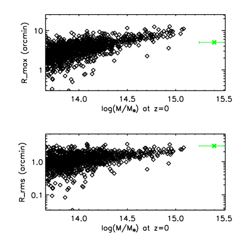
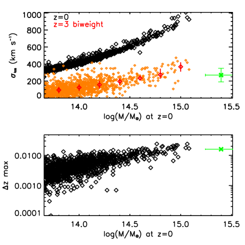
The quantities $R_{max}$ and $R_{rms}$ are shown in Fig. 3, as functions of $M_{0,sim}$, together with the values for our overdensity. The $R_{max}$ value of our overdensity (5 arcmin) has been computed using only the galaxies in P2Q1. Because of this, this value should be considered a lower limit. It is not possible to measure the real $R_{max}$, since we cannot know if the galaxies in the overall COSMOS field in the same $\Delta z$ as the overdensity (spanning the entire $RA$-$Dec$ range of the field) will collapse in one single cluster at $z=0$, because their density outside P2Q1 is consistent with the field. On the contrary, thanks to our analysis of the Millennium Simulation we expect that its $R_{max}$ will be around 10-12 arcmin (see top panel of Fig. 3), given its $M_{z=0}$. As a consequence, to derive the $R_{rms}$ of our structure we used all the galaxies within a radius of 12 arcmin from the median $RA$ and $Dec$ of the galaxies in the structure (very close to the centre of quadrant P2Q1).

The top panel of Fig. 4 shows the velocity dispersion along the line of sight ($\sigma_{los}$) as a function of the total cluster mass at $z=0$ for the clusters in the simulation. For each cluster, we plot both $\sigma_{0,sim}^{1D}$ and the $\sigma_{los}$ computed with the biweight method using the redshift of the galaxies at $z\sim 2.9$. When comparing black and orange points, it is evident that $\sigma_{los}$ increases as time goes by (as already shown in simulated clusters e.g. by Eke et al. 1998). The panel also shows that the measured velocity dispersion of our structure is below the typical $\sigma_{los}$ of proto-clusters in the simulation. In the plot, the values of $\sigma_{los}$ at $z\sim 2.9$ are computed with the biweight method using all the available galaxies. For the richest proto-clusters ($N_{z=2.9}^{gal}\geq 30$), we also measured the same $\sigma_{los}$ but using only 12 galaxies (as in our structure). We repeated this computation 1000 times per proto-cluster, and we verified that the median of the distribution of such 1000 $\sigma_{los}$ is always very close to the $\sigma_{los}$ computed using all the available galaxies, with a maximum difference of $\sim 20\,{\rm km\,s}^{-1}$.

The bottom panel of Fig. 4 is similar to the top panel in Fig. 3, but on the $y$-axis we plot $\Delta z_{max}$, i.e. the maximum range in redshift covered by the galaxies at $z\sim 2.9$. This plot is particularly useful for determining which is the more suitable redshift interval in which ‘proto-clusters’ should be searched for at $z\sim 3$. This figure suggests that searches for proto-clusters at $z\sim 3$ should be done in redshift bins of $\Delta z\lesssim 0.02$ (although this result is based on a small sample), to which the typical redshift measurement error of the given survey should be added in quadrature. In the case of VUDS, the redshift measurement error is small compared to $\Delta z\sim 0.02$ ($\sigma_{zs}=0.0005(1+z)$, see Sect. 2), so its effect is negligible.

Figure 5: HST-ACS images from the HST-COSMOS survey (Koekemoer et al. 2007), centred on the six ‘free-line-of-sight’ background galaxies (see text for details). The red circle has a radius of $6.4^{\prime\prime}$, corresponding to $50\,{\rm kpc}$ (physical) at $z=2.9$. All the other visible sources within the circle are spectroscopic galaxies with $z_{s}<2.8761$ or $z_{s}>2.9133$ or photometric galaxies with $z_{p}<2.895-0.17$ or $z_{p}>2.895+0.17$.

Table 1: Equivalent width (EW) measurements for the absorption feature at $\lambda=4736$Å, for different samples of background galaxies (all background galaxies, background galaxies with redshift flag=3 and 4, and ‘free-line-of-sight’ background galaxies). The EW is rest frame and expressed in Å. See Sect. 4 for details on the computation of the EW error and the definition of “measurement S/N” and “detection S/N”. All these quantities are computed for both the mean and median smoothed stacked spectrum.

Sample	Ngal	Mean			Median
		EW (r.f.)	S/N meas.	S/N det.	EW (r.f.)	S/N meas.	S/N det.
Bkg galaxies, flag=2,3,4	36	$4.0\pm 1.2$	3.3	3.4	$3.9\pm 1.4$	2.9	3.3
Bkg galaxies, flag=3,4	18	$5.1\pm 1.5$	3.3	3.9	$6\pm 1.8$	3.3	4.0
Bkg ‘free-line-of-sight’	6	$10\pm 2.2$	4.5	5.9	$10.8\pm 3.7$	2.9	3.9

4 Searching for diffuse cold gas

In this section we describe our search for the presence of (diffuse) cold gas within the proto-cluster. It has already been suggested that galaxies could be fed by cold gas streams. The detection and study of such gas, in the form of flows, blobs, or diffuse nebulas, would add precious pieces to the puzzle of galaxy evolution. Here, we try to give constraints on the presence of this gas by examining the absorption features in the spectra of galaxies in the background of our structure, as already done, for example, in Giavalisco et al. (2011) for an overdensity at $z=1.6$. We discuss our results in Sect. 6.

We inspected the spectra of the galaxies in the background of the structure, searching for an absorption feature at the wavelength of the Ly$\alpha$ at $z=2.895$, i.e. $\lambda=4736$Å. Our aim is to verify the presence of gas in the halo of the galaxies in the overdensity or diffuse gas in the IGM of the overdensity itself.

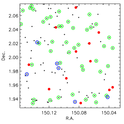
These background galaxies are selected to be at $3\leq z\leq 4.15$, with secure $z_{s}$ (flag=2, 3, 4, 9), and observed in the same VIMOS quadrant as the structure. The lower limit in $z_{s}$ is required to distinguish the possible absorption by Ly$\alpha$ at $z=2.895$ from the intrinsic absorption of the Ly$\alpha$ in the given background galaxy. The upper $z_{s}$ limit excludes galaxies for which the line at $\lambda=4736$Å  (observed) falls blue-wards of the Lyman limit at 912Å  (rest frame). For such galaxies, we would not have signal in the wavelength range of interest. With this selection, we found 36 background galaxies, amongst which 18, 12, and 6 with flag =2, 3, and 4 respectively. We also found one broad-line AGN with a secure redshift, which we do not use in our analysis.

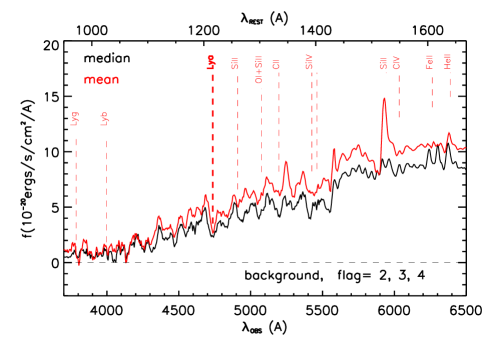
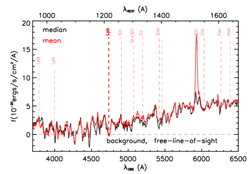
The top panel of Fig. 6 shows the mean and median stacked spectrum of all the 36 background galaxies at observed wavelengths. We compute the stacked spectrum in the following way. We interpolate each input spectrum on the same grid with a pixel scale of 5.3Å/pixel (i.e. the dispersion of the blue grism used for the observations). Even if the pixel scale is the same as in each single spectrum, each of the spectra is interpolated on this pixel scale before co-adding, and the flux rescaled to preserve the total flux after rescaling. For each of the spectra, we compute the median sky level, and we consider ‘good pixels’ to be those for which the sky flux is within 120% of the median sky level. In this way, in each spectrum, we exclude the regions contaminated by strong sky lines from the analysis. For each grid pixel at $\lambda_{i}$, the flux $f_{i}$ in the co-added spectrum is computed as the median (or mean) of the fluxes at $\lambda_{i}$ of the input spectra, where only spectra for which the pixel at $\lambda_{i}$ is a good pixel were considered. For each $\lambda_{i}$, we retain the information on the number of spectra that have been used for the stacking ($N_{s,i}$). The stacked spectrum is then smoothed on a scale comparable to the resolution of VUDS spectra at the line of interest. Given R=230 (see Sect. 2), we obtain a resolution element of $\Delta\lambda\sim 25$Å  at $\lambda=4736$Å. Spectra are neither normalised nor weighted before stacking.

In the spectra showed in Fig. 6 we do see an absorption feature at $\lambda=4736$Å. In the median spectrum, this absorption feature has a rest frame FWHM $\sim 9$Å  (not deconvolved with instrumental resolution) and rest frame equivalent width ${\rm EW}\sim 4\pm 1.4$Å, i.e. a measurement S/N of $\sim 3$. Its detection S/N is $\sim 3.3$. The error on the EW has been computed in a similar way to Tresse et al. (1999). For the mean spectrum we obtain very similar values (see Table 1). If we stack only the background galaxies with redshift flag=3 and 4 (mid panel in Fig. 6), we find slightly larger EW in both the mean and median spectra, but the values are compatible with the ones obtained by stacking all galaxies (see Table 1).

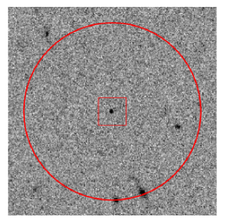
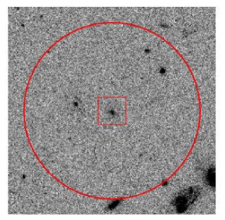
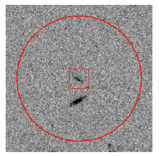
Given that this feature is detected in both the mean and median spectra with a reasonable S/N, this suggests that it is a common feature in the sample of background galaxies and not due to a minority of the spectra. This absorption feature is also visible (by eye) in some of the single spectra. Clearly, this absorption could be caused by the presence of an intervening galaxy in the structure and not to diffuse gas. For instance, inspecting the HST image of the galaxy where the absorption line at $\lambda=4736$Å  is the most evident, we notice that there are two faint objects close to the galaxy without any spectroscopic or photometric redshift, one of the two possibly belonging to the galaxy itself. In such a case it is not possible to say if the absorption at $\lambda=4736$Å  is due to diffuse gas at $z\sim 2.895$ or to one of the two faint objects, which could be at $z\sim 2.895$.

To have a better handle on the possibility of detecting diffuse gas, we removed this and similar cases from our background sample in the following way. We looked in a radius of $50\,{\rm kpc}$ (physical) around each background galaxy and removed the given background galaxy from our analysis if in that radius i) there was another VUDS galaxy with $2.8761\leq z_{s}\leq 2.9133$; ii) there was a galaxy with $z_{p}$ (primary or secondary peak) in the range $z=2.895\pm 0.17$; iii) there was one or more unidentified sources (not included in our photometric catalogue) in the HST image. A possible absorption found in a background galaxy at $\lambda=4736$Å, even if caused by gas at $z\sim 2.895$, would not be resolved from an absorption line due to a foreground galaxy in the range $2.8761\leq z_{s}\leq 2.9133$ (given the resolution of the grism), and this consideration gives us the restriction on spectroscopic galaxies assumed in point i). For galaxies with only $z_{p}$ (point ii), we computed the distribution of $z_{s}-z_{p}$ for galaxies with $2.5<z_{s}<3.5$, fitted it with a Gaussian function and found $\sigma\sim 0.17$, which we used as the redshift interval assumed in point ii).

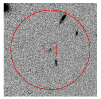
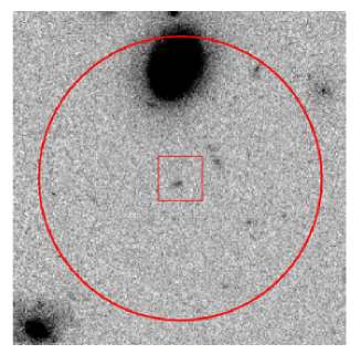
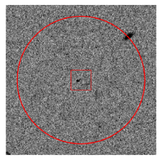
After removing the background galaxies satisfying these three criteria, we are left with six ‘free-line-of-sight’ background galaxies. They are in the range $3.1\lesssim z_{s}\lesssim 4.1$, and are distributed quite uniformly in $RA$-$Dec$, covering half of the entire sky area of the structure (see bottom panel of Fig. 1). Figure 5 shows the HST images centred on these six galaxies. Their median and mean coadded spectra are shown in the bottom panel of Fig. 6. In the median spectrum, the absorption line at $\lambda=4736$Å  has a flux detection S/N of about 4 and a rest frame ${\rm EW}\sim 11\pm 4$Å, i.e. an EW measurement S/N of $\sim 3$. The rest frame FWHM is $\sim 10$Å.

In the stacked spectrum of the six ‘free-line-of-sight’ galaxies there are no other absorption features with a meaningful EW corresponding to typical lines at $z=2.9$, but one. This exception is the (blended) doublet Si IV $\lambda\lambda 1393,1402$, with a rest frame EW of $5.5\pm 1.5$Å. This absorption feature is also visible in the two other panels of Fig. 6, but with a lower EW ($\sim 3\pm 1$Å). We also estimated the EW of the blends OI - Si II $\lambda\lambda 1302,1304$, and C II $\lambda 1334$ in the coadded spectrum of galaxies with redshift flag=3 and 4, and we find ${\rm EW}\sim 3\pm 1$ and ${\rm EW}\sim 2\pm 1$Å, respectively. Nevertheless, the lines are blended, and they become even less evident when also coadding flag 2 and 9.

We verified that the absorption line at $\lambda=4736$Å  in the observed frame coadded spectrum of the six ‘free-line-of-sight’ galaxies is not a spurious effect of the noise of the coadded spectra. We did this by comparing its EW with the EW of all the possible absorption features (real or not) in 1000 stacked spectra, obtained by stacking six galaxies chosen randomly amongst all the VUDS galaxies in the COSMOS field, with redshift quality flag equal to 2, 3, 4, and 9, and with $z_{s}\geq 3$. The result of this test does not change when the sets of six galaxies are built considered only galaxies in the same redshift range as the six galaxies with a free line of sight, i.e. $3.14\leq z\leq 4.12$.

Appendix A describes in detail how we computed the distribution of the observed-frame EWs of all the absorption features in these 1000 stacked spectra. We find that the $25^{th}$, $50^{th}$, and $75^{th}$ percentile of this distribution correspond to 3.6, 7.3, and 12.6Å. The observed frame EW of the absorption line in the median stacked spectrum of our six galaxies is 42Å. This value corresponds to the $99^{th}$ percentile of the distribution of all the absorption features in the 1000 stacked spectra. This result suggests that our measurement is unlikely to be due to noise fluctuations. Moreover, in this analysis we did not make any use of the additional information that the detected absorption line at $\lambda=4736$Å  is exactly at the wavelength corresponding to $Ly\alpha$ absorption at the redshift of the structure. This fact reduces the likelihood that this line is spurious even further. The physical interpretation of this significant feature is discussed in Sect. 6.2.

5 Galaxy properties

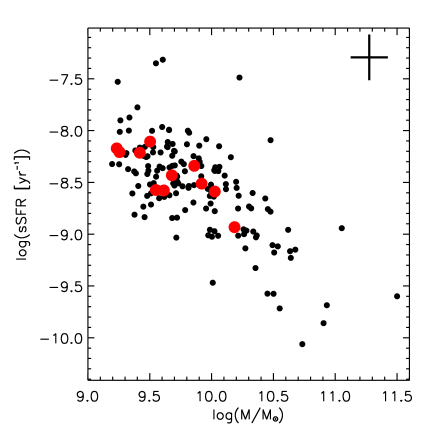
In this section we analyse the properties of the galaxies within the overdensity, and we compare them with a control sample at the same redshift but outside the overdensity. For this analysis, we use only galaxies with redshift quality flag=3 and 4, so in the overdensity we retain only 11 galaxies out of 12 (see Sect. 3). The control sample comprises all the VUDS galaxies with flag=3 and 4 in the range $2.8<z<3.0$, outside the structure. This sample includes 151 galaxies. In the following analysis, we include all the galaxies in the two samples, irrespective of their stellar mass $\mathcal{M}$. We verified that the results do not change if we use only galaxies above a given mass limit, common to the two samples (i.e. ${\rm log}_{10}(\mathcal{M}/M_{\odot})\geq 9.5$).

A more detailed analysis is deferred to a future work, when the VUDS selection function (Tasca et al, in prep.) will be fully assessed. A robust computation of the selection function will allow us to quantify the selection biases against specific population(s) due to the VUDS observational strategy (such as the most massive and passive galaxies, as described in Sect. 2.1). Nevertheless, we note that here we perform a differential comparison of two samples observed with the same strategy, and we do not attempt to compare our results here in an absolute way with other samples from the literature.

We also stress that, given the small sample (11 galaxies in the overdensity), the comparison of the galaxies in the overdensity with any control sample is prone to large uncertainties. This kind of analysis is better performed with larger samples of galaxies, but the analysis presented here has the advantage of being one of the few ever attempted at these high redshifts.

5.1 Stellar mass, star formation, and colours

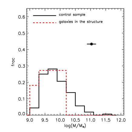
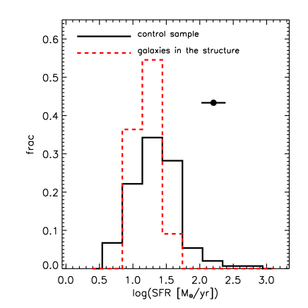
Figure 7 shows the distribution of $\mathcal{M}$ and SFR for the two samples. Both $\mathcal{M}$ and SFR are computed via SED fitting (see Sect. 2.1). On the basis of a KS test, in both cases, the two distributions are consistent with being drawn from the same $\mathcal{M}$ and SFR distributions. As a complementary test, we also verified the probability that a random sample of 11 galaxies, extracted from the control sample, could lack the high-mass tail, as we find in the proto-cluster (see the top panel of Fig. 7). We randomly extracted 11 galaxies 1000 times from the control sample, which has a maximum $\mathcal{M}$ of ${\rm log}_{10}(\mathcal{M}/M_{\odot})\sim 11.5$. We found that, over the 1000 extractions, the maximum $\mathcal{M}$ has a mean value of ${\rm log}_{10}(\mathcal{M}/M_{\odot})\sim 10.6$ with a dispersion of 0.35. This means that the maximum $\mathcal{M}$ found in the proto-cluster (${\rm log}_{10}(\mathcal{M}/M_{\odot})\sim 10.2$) is only $1.2\sigma$ lower than the typical extracted one, confirming the result of the KS test.

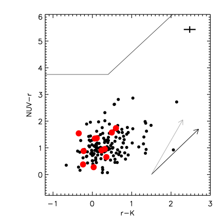
The top panel of Fig. 8 shows the $(NUV-r)$ vs $(r-K)$ rest frame colours. This plot is particularly useful for distinguishing between active and passive galaxies, since it is able to distinguish dusty active galaxies from truly red and passive ones (see e.g. Williams et al. 2009; Arnouts et al. 2013). Namely the $NUV-r$ colour is sensitive to specific star formation (sSFR: the higher the sSFR, the bluer the colour), because $NUV$ traces recent star formation and $r$ the old stellar populations. Dust attenuation can alter the $NUV-r$ colour, moving dusty star-forming galaxies towards redder colours. The $r-K$ colour does not vary much for different stellar populations, but is very sensitive to dust attenuation (see e.g. Fig. 3 in Arnouts et al. 2013). Using both colours, it is possible to partially disentangle red passive galaxies from dusty active ones. The top panel of Fig. 8 shows that possibly the galaxies in the structure have a bluer $r-K$ colour (perhaps meaning that are less attenuated by dust), but, given the lack of statistics, the difference in the $r-K$ distribution between the two samples is not significant on the basis of a KS test. We note that the locus of passive galaxies defined in Arnouts et al. (2013) is $(NUV-r)>3.75$ for $(r-K)<0.4$ and $(NUV-r)>1.37\times(r-K)+3.2$ for $(r-K)\geq 0.4$; i.e., it corresponds to $NUV-r$ colours that are much redder than we find in our sample.

The bottom panel of Fig. 8 shows the sSFR versus the stellar mass. Also in this case, the galaxies in the structure do not seem to have very different properties from those in the control sample. At most, they could show a less scattered relation between sSFR and $\mathcal{M}$, but given the error on the sSFR computation (see the cross in the top right corner of the panel), this difference is not significant.

We also analysed how galaxies are distributed in the plane $J-K$ vs $K$ (observed magnitudes). The filters $J$ and $K$ bracket the D4000Å  break at $z\sim 3$, so the $J-K$ colour can be used to identify passive galaxies (see e.g. Hatch et al. 2011). We found that galaxies within and outside the structure are distributed very similarly in the $J-K$ vs $K$ plane. The reddest galaxies do not belong to the overdensity, but to the field, and they do not seem to reside primarily in the proximity of the overdensity. Considering the two reddest spectroscopic galaxies in the structure, which have a very similar $J-K$, one is located in the middle of P2Q1, the other one close to its boundary.

In summary, we do not find any significant difference between the colours, stellar masses, SFR, and sSFR of the galaxies in the proto-cluster and in the control sample. While we cannot exclude that the lacking of any difference is real, it might also be due to the lack of statistics, or to the fact that we miss, in our sample, a particular galaxy population that environment could affect more strongly (see e.g. the most passive galaxies, as discussed at the end of Sect. 2.1). A more careful analysis of this possible selection bias is deferred to a future work.

Figure 6: Top. Median (black) and mean (red) stacked spectrum of all the background galaxies at observed wavelengths. Middle. Same as top panel, but stacking only background galaxies with redshift flag = 3 and 4. Bottom. Same as top panel, but stacking only the six ‘free line-of-sight’ background galaxies (see text for details).

5.2 Stacked spectra

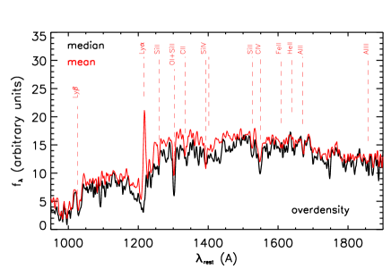
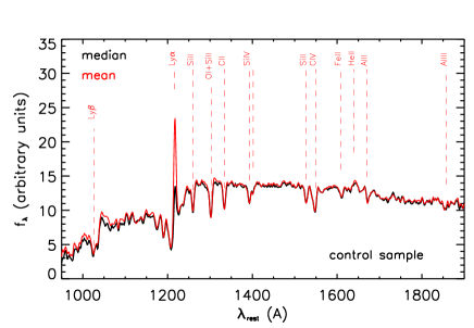
Figure 9 shows the stacked spectra of the two subsamples of galaxies, i.e. the 11 galaxies in the overdensity (top panel) and the 151 galaxies in the control sample (bottom panel). Spectra are stacked as in Sect. 4, but in this case they have been blue-shifted to rest frame wavelength before stacking, and the stacked spectrum is smoothed with a Gaussian filter with $\sigma$ equal to one pixel.

The two spectra show some differences. First, the median stacked spectrum of the control sample shows some Ly$\alpha$ in emission, indicating that at least half of the galaxies in the control sample have Ly$\alpha$ in emission, while this is not the case for the median spectrum of the galaxies in the overdensity. We verified that only 3 out of these 11 galaxies show an emission line at $\lambda=1216$Å  (rest frame). However, given the low statistics, this result does not give us any clue to the typical Ly$\alpha$ in the galaxies in the overdensity, given that the number of galaxies with Ly$\alpha$ in emission in the structure is compatible, at $2\sigma$ level, with being more than 50%. In more detail, the three Ly$\alpha$ emitters in the proto-cluster have an EW(Ly$\alpha)>25$Å  rest frame, which makes them strong emitters according to the definition in Cassata et al. (2014). This means that the strong emitters are $27\pm 13$% of the proto-cluster sample. In the control sample, we find $19\pm 3$% of strong Ly$\alpha$ emitters. The two fractions both agree, within the error bars, with the overall percentage of strong Ly$\alpha$ emitters at $z=3$ found in Cassata et al. (2014) for the entire VUDS sample.

In the control sample coadded spectrum all the ISM absorption lines are clearly visible: Si II $\lambda 1260$, the blend OI - Si II $\lambda\lambda 1302,1304$, C II $\lambda 1334$, the doublet Si IV $\lambda\lambda 1393,1402$, Si II $\lambda 1526$, the doublet C IV $\lambda\lambda 1548,1550$, Fe II $\lambda 1608$ and Al II $\lambda 1670$. Despite the higher noise, all these lines are also visible in the coadded spectrum of the overdensity galaxies, with the exception of Fe II $\lambda 1608$. The fact that we do not see a clear Fe II $\lambda 1608$ absorption is probably because it falls in a region where the observed frame spectrum is contaminated by sky lines: the 11 galaxies in the structure are almost at the same redshift, so the observed frame skylines in the 11 spectra always fall in the same rest-frame wavelength. This does not happen for the galaxies in the control sample, which span a larger extent in redshift. All the absorption lines in the proto-cluster coadded spectrum have EWs that are compatible, within the error bars, with those in the coadded spectrum of the control sample.

Figure 7: Top. Distribution of galaxy stellar masses in the control sample (black solid line) and in the structure (red dashed line). Bottom. Same as in the top panel, but for the distribution of SFR. In both panels, the solid point with the error bar shows the typical error on $\mathcal{M}$ and SFR. The possible systematic offset in the SFR computation due to the choice of different SFHs (see Sect. 2.1) is not included.

Figure 8: Top. $NUV-r$ vs $r-K$ rest frame colours. Black dots are the control sample, red filled circles are the galaxies in the structure. The solid thick lines comprise the locus of passive galaxies defined in Arnouts et al. (2013). The two arrows represent the attenuation vectors for starburst (dark arrow) and Small Magellanic Cloud (light arrow) attenuation curves assuming $E(B-V)=0.4$ as in Arnouts et al. (2013) (see their Fig.2). Bottom. sSFR versus stellar mass. Symbols as in the top panel. In both panels, the cross in the top right corner shows the typical error on the quantities plotted on the two axes. The possible systematic offset in the SFR computation due to the choice of different SFHs (see Sect. 2.1) is not included when deriving the error on the sSFR.

Figure 9: Top: coadded spectrum of the 11 galaxies in the structure with redshift quality flags 3 and 4. Bottom: coadded spectrum of the 151 galaxies in the control sample with redshift quality flags 3 and 4. Line and colour codes are as in Fig. 6.

6 Discussion

The overdensity that we found at $z\sim 2.9$ in the VUDS sample in the COSMOS field has two main characteristics that make it an extremely interesting case study: the high value of the galaxy overdensity and the evidence of the presence of cold gas in the IGM. In this section we discuss in more details these two points.

6.1 The overdensity

In Sect. 3, we estimated a galaxy overdensity of $\delta_{g}=12\pm 2$. This overdensity is much higher than the typical $\delta_{g}$ found in the literature at similar redshift (e.g. $\delta_{g}\sim 6$ at $z=3.09$ in Steidel et al. 2000, $\delta_{g}=2.3$ at $z=3.13$ in Venemans et al. 2007; see also Table 5 in Chiang et al. 2013 for a more complete list, and their more recent work shown in Chiang et al. 2014). Overdensities with $\delta_{g}$ similar to ours have been found, but they are very rare, and they seem to span a wide redshift range (e.g. $\delta_{g}\sim 8.3$ at $z=1.6$ in Kurk et al. 2009, $\delta_{g}\sim 16$ at $z\sim 6$ in Toshikawa et al. 2012). We also refer the reader to Lemaux et al. (2014), where we study a spectroscopic overdensity of $\delta_{g}=13.3\pm 6.6$ found at $z=3.3$ in the VVDS field using VUDS observations.

The study of such over-dense regions is particularly important because these structures are more likely to become clusters than are lower density structures (Chiang et al. 2013). This allows us to study how mass assembles along cosmic time. In our case, the high $\delta_{g}$ value is primarily due to the narrow $z$ range ($\Delta z=0.016$) in which the spectroscopic members reside compared with much larger redshift slices in which other overdensities have been found.

The large $\delta_{g}$ means a high total mass (given the typical bias between galaxies and matter at $z=2.9$). Specifically, we find that the total mass associated to the structure at $z=2.9$ is $\sim(8.1\pm 2.4)\times 10^{14}M_{\sun}$, which makes our overdensity one of the most massive found in the literature at high redshift. Following Chiang et al. (2013), we estimate that this structure will collapse in a cluster with $M_{z=0}\sim(2.5\pm 0.8)\times 10^{15}M_{\odot}$ at $z=0$. For both masses, the uncertainty represents $\sim 30$% of the nominal value (see Sect. 3.2). We verify how rare these structures might be and how many we should expect to find in the volume explored by VUDS in the COSMOS field. Considering the snapshot at $z=0$ of the Millennium Simulation, we find a density of $(1.1\pm 0.5)\times 10^{-8}$ clusters/Mpc³ for clusters with $M_{z=0}\sim(2.5\pm 0.8)\times 10^{15}M_{\odot}$. This result is in rough agreement with the cluster mass function at $z\sim 0$ in Vikhlinin et al. (2009) (see their Fig. 1): in their work, the density of clusters with mass $M_{z=0}\sim(2.5\pm 0.8)\times 10^{15}M_{\odot}$ (converting their M₅₀₀ in M₂₀₀, to be consistent with the mass in the Millennium Data Base) is $\sim(2.5\pm 0.9\times 10^{-8}$Mpc^-3. Given this density range ($\sim(1.1-2.5)\times 10^{-8}$Mpc^-3), we expect to find 0.1-0.3 proto-clusters with such $M_{z=0}$ in the volume covered by VUDS in the COSMOS field in the entire redshift extent $2<z<3.5$.

At face value, the measurement of a total mass of $\sim 8\times 10^{14}M_{\sun}$ at $z\sim 2.9$ and a total mass of $\sim 2.5\times 10^{15}M_{\sun}$ at $z=0$ seems to suggest a very small evolution in mass. This is not true, since the two masses are not directly comparable. The mass measured at $z=0$ is the mass bound in the cluster, while at $z\sim 2.9$ we measure the total mass that will collapse in that cluster and that at $z\sim 2.9$ is not necessarily bound in one single structure. The two masses should differ only by the factor $C_{e}$ described by Chiang et al. (2013), which links the total mass at $z\sim 2.9$ enclosed in a given volume with the final bound mass at $z=0$. The most evident evolution from the overdensity at $z\sim 2.9$ and its descendant cluster at $z=0$ is an evolution in overdensity and not in total mass.

A different discussion has to be devoted to the measured velocity dispersion. We measured $\sigma_{los}=270\pm 80\,{\rm km\,s}^{-1}$ with the biweight method, a method that is quite effective in measuring a dispersion of a contaminated Gaussian distribution. Indeed, it is not known which should be the shape of the velocity distribution of galaxies in a proto-cluster, if such structure is not already relaxed. We inspected the shape of the velocity distribution of the galaxies in the proto-clusters at $z=2.9$ in the galaxy mock catalogues that we used in Sect. 3.3, focusing our attention on the proto-clusters that will collapse in clusters with $M_{z=0}\gtrsim 10^{15}M_{\odot}$. We found that these velocity distributions can have a broad range of shapes, from Gaussian, to contaminated Gaussian, to almost flat distributions. Indeed, if our measured $\sigma_{los}$ is lower than the expected one (see Eke et al. 1998), there are cases in the literature where the measured $\sigma_{los}$ is too large with respect to expectations (see e.g. Toshikawa et al. 2012). We suggest that the important piece of information that we can retrieve from simulations is the maximum span in redshift space that the member galaxies can encompass, rather than their velocity dispersion. The first one is needed to tune the search for high-$z$ overdensities, while the second one might be less meaningful, depending on the evolutionary state of the proto-cluster under analysis.

6.2 The diffuse gas

The stacked spectrum of the background galaxies at $z>3.0$ shows an absorption consistent with Ly$\alpha$ at z = 2.895 ($\sim 4736\AA$). Its rest frame EW is $\sim 4-10$Å  according to the sample used for the stacking (see Table 1). These EWs correspond to N(HI) $\sim 3-20\times 10^{19}$cm^-2 (with large uncertainties and assuming a constant gas density over the transverse dimension of the structure). The angular size of the structure would imply a total mass of HI of a few $10^{12}-10^{13}M_{\odot}$ if the absorption were due to diffuse gas.

Several hypotheses can be suggested on the very nature of this absorption feature. The debate is open in the literature about the detectability of the signature of physical processes that could give rise to such a feature. The first hypothesis, already introduced above for the computation for the total HI mass, is that the Ly$\alpha$ in absorption is related to the diffuse gas (IGM) within the overdensity. This could be the case especially for the six ‘free-line-of-sight’ galaxies, because they are $>50\,{\rm kpc}$ (physical) away from all the identified sources in the structure.

The high column density that we infer could support a second hypothesis that the absorption is due to intervening cold streams of gas, which are falling into the potential well of the galaxies in the overdensity. This high column density is shown, for instance, in Goerdt et al. (2012). They use hydrodynamical simulations at $z\sim 3$ to create and trace such streams in the circumgalactic medium via Ly$\alpha$ absorption manifest in the spectra of background galaxies. In particular, their Fig. 15 shows that the projected HI column density of such absorption features can reach up to a few $10^{20}$cm^-2 at a distance of more than $50\,{\rm kpc}$ from the galaxy that is fed by cold streams. This N(HI) value is consistent with the N(HI) of the absorption line that we find in the stacked spectrum of the ‘free-line-of-sight’ background galaxies. Similarly, they show in their Fig. 20 that the Ly$\alpha$ rest frame EW can easily reach values of ${\rm EW}\sim 4-5$Å  along the line of sight of the cold flows up to $60-80\,{\rm kpc}$ from the centre of the galaxy.

The fraction of the area (or ‘covering factor’) around a galaxy that is covered by these cold streams with high enough density to produce a detectable absorption line is very low. For ${\rm EW}({\rm Ly}\alpha)\sim 4-5$Å, Goerdt et al. (2012) show that the covering factor is typically a few percent. Given these results for the covering factor, the fact that we see such a strong absorption not only in the mean stacked spectrum, but also in the median, strongly suggests that the absorption is due to a more widely extended source rather than to cold streams. On the other hand, the fact that we are studying an over-dense region would likely give rise to denser and/or more widely distributed filaments (see e.g. Kimm et al. 2011, who find that the covering fraction of filaments is larger in more massive haloes).

Very similar results for simulated cold streams extension, N(HI), and covering factor are shown in Fumagalli et al. (2011) (see e.g. their Fig 6). They also show that such cold flows are generally metal poor (as also shown in Goerdt et al. 2012 and Kimm et al. 2011). They suggest that any observational detection of metal lines is more probably due to outflows rather than infalls. We do not find any other significant absorption lines in the coadded spectrum of the ‘free-line-of-sight’ background galaxies except for the Si IV $\lambda\lambda 1393,1402$ (blended) doublet, with a rest frame EW of $5.5\pm 1.5$Å  (EW $=3\pm 1$Å  for the total sample of background galaxies). Such an EW could, however, be because this is a not resolved doublet. This detection, which does not directly support the infall scenario, will deserve further analysis.

7 Summary and conclusions

In this work, we have characterised a massive proto-cluster at $z=2.895$ that we found in the COSMOS field using the spectroscopic sample of the VUDS survey. Our results can be summarised as follows:

• The overdensity comprises 12 galaxies with secure spectroscopic redshift in an area of $\sim 7^{\prime}\times 8^{\prime}$, in a total redshift range of $\Delta z=0.016$. The measured galaxy overdensity is $\delta_{g}=12\pm 2$. According to simulations (Chiang et al. 2013), a structure with $\delta_{g}=12$ at $z\sim 2.9$ has a 100% probability of evolving into a galaxy cluster at $z=0$.

• We estimated that this overdensity has a total mass of $M\sim 8.1\times 10^{14}M_{\odot}$ in a volume $13\times 15\times 17$ Mpc³. According to Chiang et al. (2013), such an overdensity should collapse into a cluster of total mass $M_{z=0}\sim 2.5\times 10^{15}M_{\odot}$ at $z=0$. In the volume surveyed by VUDS at $2<z<3.5$ in the COSMOS field, we should have expected 0.12-0.3 proto-cluster of this kind.

• The velocity dispersion of the 12 members is $\sigma_{los}=270\pm 80\,{\rm km\,s}^{-1}$. We used light cones extracted from the Millennium Simulation to verify that this is lower (but consistent within $2\sigma$) than the typical velocity dispersion of the galaxies belonging to the same kind of proto-clusters at this redshift. This low value is consistent with the increase in $\sigma_{los}$ as time goes by (Eke et al. 1998).

• In the light cones that we examined, the typical span in redshift of the galaxies belonging to proto-clusters at $z\sim 2.9$, which will collapse into massive clusters at $z=0$, is $\Delta z\sim 0.02$. This value is much lower than the redshift bin often used to search for proto-clusters at this redshift.

• The stacked spectra of the galaxies in the background of the overdensity show a significant absorption feature at the observed wavelength corresponding to the Ly$\alpha$ at the redshift of the structure ($\lambda=4736$Å). We find that this absorption feature has a rest frame EW of $10.8\pm 3.7$Å, with a detection S/N of $\sim 4$, when stacking only background galaxies without intervening sources at $z\sim 2.9$ along their line of sight. We verified that this measurement is likely not to be due to noise fluctuations. Considering also the lower (but consistent) EW found using different samples of background galaxies (see Table 1), such an EW range corresponds to a column density N(HI) of the order of $3-20\times 10^{19}$cm^-2.

• We analysed the properties of the galaxies within the overdensity, and we compared them with a control sample at approximately the same redshift outside the overdensity. We could not find any statistically significant difference between the properties (stellar mass, SFR, sSFR, $NUV-r$, $r-K$) of the galaxies inside and outside the overdensity, but this result might be due to the lack of statistics, or possibly to the specific galaxy population sampled by VUDS, which could be less affected by environment than other populations not probed by the survey.

Simulations (Chiang et al. 2013) indicate that such an overdensity at $z\sim 2.9$ is indeed a proto-cluster that, given the measured galaxy overdensity, will collapse to a (massive) cluster at $z=0$. For this reason, the detailed analysis of this proto-cluster represents a fundamental step in the comprehension of galaxy formation and evolution.

For the properties of the galaxies within the proto-cluster, we plan to do a more detailed study when the VUDS selection function is assessed. A well-defined selection function will allow us to robustly quantify the average properties of the galaxies in such a dense environment and to compare them with the galaxies in the field at the same $z$ and with other overdensities found in the literature (e.g. Lemaux et al. 2014). The synergy of spectroscopy and multi-band photometry in next-generation surveys like Euclid will allow several proto-cluster structures to be identified thanks to combination of depth and large surveyed areas. In this respect, current surveys such as VUDS, are essential for characterising the properties of these structures and using them to predict their observability and optimal detection with future surveys.

On the side of the detection of cold gas, the EW of the absorption line corresponding to the Ly$\alpha$ at $z\sim 2.9$ implies a high column density (N(HI)$\sim 10^{20}$cm^-2). This N(HI) value would be compatible with the scenario where the absorption is due to intervening cold streams of gas, which are falling (and feeding) into the halo’s potential well of the galaxies in the proto-cluster (Fumagalli et al. 2011; Goerdt et al. 2012). In contrast, the stacked spectrum of the galaxies in the proto-cluster background also shows an absorption line corresponding to Si IV $\lambda\lambda 1393,1402$ (blended) doublet at the redshift of the proto-cluster, detection that does not agree with the prediction that the cold flows are metal poor. Surely, the scenario of gas accretion by cold gas stream needs to be more robustly assessed from additional observational evidence. An exciting prospect is to look for the Ly$\alpha$ emission produced by gravitational energy released by cold gas flowing into the potential wells of galaxies (see e.g. Goerdt et al. 2010).

Appendix A Testing the robustness of the absorption line

We implemented an automatic procedure to measure the EW of all the absorption features (real or not) in a homogeneous way in the 1000 stacked spectra mentioned at the end of Sect. 4. Specifically, we performed the following analysis at each pixel (at position $\lambda_{i}$) of the stacked spectrum. We define the continuum $f_{c,i}$ around $\lambda_{i}$ as the mean value of the flux of the coadded spectrum in the two intervals $\lambda_{i}-280<\lambda<\lambda_{i}-80$Å  and $\lambda_{i}+80<\lambda<\lambda_{i}+280$Å. To compute the mean, we use only the pixels where $N_{s,i}\geq 4$ (see Sect. 4 for the definition of $N_{s,i}$). If the flux $f_{i}$ at $\lambda_{i}$ is above $f_{c,i}$, there is no absorption line at that position, so we move to the next $\lambda_{i}$. If $f_{i}$ is below $f_{c,i}$, we compute the ${\rm EW}_{i}$ of the possible line centred at $\lambda_{i}$, considering as ‘line’ the spectrum in the range $\lambda_{i}-30<\lambda<\lambda_{i}+30$ Å.

The output of this procedure is a value of EW_i for each $\lambda_{i}$ with $f_{i}<f_{c,i}$ in the coadded spectrum. By definition, ${\rm EW}_{i}$ is positive for absorption features and negative for emission features. In our analysis, we keep only the ${\rm EW}{\rm s}_{i}$ that satisfy the following requirements:

• ${\rm EW}_{i}$ must be positive.

• The continuum around the line must be entirely included in the observed spectrum, so we need $(\lambda_{i}-280)>3600$Å  and $(\lambda_{i}+280)<9350$Å.

• The flux at $\lambda_{i}$ must be a local minimum, i.e. $f_{i}<f_{i-1}$ and $f_{i}<f_{i+1}$. In the majority of cases, $f_{i}$ is less than $f_{c,i}$ only because of noise fluctuations around the continuum, and most probably $f_{i-1}$ and $f_{i+1}$ will be above the continuum. We want to keep all these cases. In the case of absorption features larger than one pixel and centred at a given $\lambda_{c}$, $f_{i}$ will be below the continuum for $\lambda_{i}$ included in a given range $[\lambda_{c}-L,\lambda_{c}+L]$, where $2L$ is the width of the absorption feature at the level of the continuum. Our automatic procedure computes the EW centred at all possible $\lambda_{i}$ included in this range, and the output is a series of positive ${\rm EW}_{i}$ with (most probably) a (local) maximum EW at $\lambda_{c}$. We retain only ${\rm EW}_{i}$ values where $f_{i}$ is a local minimum, thus normally we keep the largest possible EW for each absorption feature.

• $N_{s,i}$ in the entire range $\lambda_{i}-30<\lambda<\lambda_{i}+30$ Å  must be $\geq 5$.

• The continuum flux $f_{c,i}$ must be computed in a range of at least 100Å. As described above, $f_{c,i}$ is measured using two intervals of $\sim 200$Å  each, but using only the fluxes $f_{i}$ where $N_{s,i}\geq 4$. In some case, this threshold shrinks the wavelength range on which $f_{c,i}$ is computed, especially at $\lambda>6000$, where the sky level in VUDS spectra is on average quite high because of fringing.

• The continuum measured on the left ($f_{c,i}^{l}$) and on the right ($f_{c,i}^{r}$) of $\lambda_{i}$ must be similar. Namely, max($f_{c,i}^{l}/f_{c,i}^{r}$, $f_{c,i}^{r}/f_{c,i}^{l}$) $\leq 1.5$. In this way we avoid absorption features that are too close to a break in the continuum, a situation difficult to be treated properly when measuring EW automatically for all features, without knowing their position and the shape of the continuum around them in advance.

The EW distribution used for the analysis at the end of Sec. 4 is computed using all the EWs in the 1000 coadded spectra that satisfy the conditions listed above. We verified that these conditions are also satisfied by the absorption line at $\lambda=4736$Å  in the stacked spectra shown in Fig. 6.