Spitzer IRS Observations of the XA Region in the Cygnus Loop Supernova Remnant

Abstract

We report on spectra of two positions in the XA region of the Cygnus Loop supernova remnant obtained with the InfraRed Spectrograph on the Spitzer Space Telescope. The spectra span the 10–35 $\mu$m wavelength range, which contains a number of collisionally excited forbidden lines. These data are supplemented by optical spectra obtained at the Whipple Observatory and an archival UV spectrum from the International Ultraviolet Explorer. Coverage from the UV through the IR provides tests of shock wave models and tight constraints on model parameters. Only lines from high ionization species are detected in the spectrum of a filament on the edge of the remnant. The filament traces a 180 km s^-1 shock that has just begun to cool, and the oxygen to neon abundance ratio lies in the normal range found for Galactic H II regions. Lines from both high and low ionization species are detected in the spectrum of the cusp of a shock-cloud interaction, which lies within the remnant boundary. The spectrum of the cusp region is matched by a shock of about 150 km s^-1 that has cooled and begun to recombine. The post-shock region has a swept-up column density of about $1.3\times 10^{18}$ cm^-2, and the gas has reached a temperature of 7000 to 8000 K. The spectrum of the Cusp indicates that roughly half of the refractory silicon and iron atoms have been liberated from the grains. Dust emission is not detected at either position.

1 Introduction

Supernova remnants (SNRs) play an important role in the life-cycle of dust in the interstellar medium (ISM). As SNR shock waves sweep up interstellar material they heat the gas and dust, and they destroy a significant fraction of the grains, whereby refractory elements are released back into the gas phase. The shock-heated dust emits strongly at infrared (IR) wavelengths and is the major contributor to the total IR flux from remnants (Arendt, 1989; Saken, Fesen & Shull, 1992). The IR wavelength regime also contains a number of collisionally excited lines that are emitted by radiative shocks. These lines provide diagnostics for the gas-phase elemental abundances, and a comparison of refractory and non-refractory species can yield a measurement of the efficiency of grain destruction. Thus, IR observations of SNR shocks are crucial for studying the dust destruction process in shocks, and useful for studying the shock properties. Most SNRs in the Galaxy are highly extincted and they cannot be detected at ultraviolet or even optical wavelengths, and in those cases the IR emission offers the only way to study the radiative shocks.

The Cygnus Loop, a middle-aged remnant, is an ideal object for the study of SNR shocks. It is bright and it is nearby, so the emitting regions can be studied at high spatial resolution. It is located away from the Galactic mid-plane and the foreground extinction is low, and is therefore observable in the ultraviolet and far-ultraviolet wavelength regimes.

The Cygnus Loop exhibits a classical shell morphology at all wavelengths. In the IR, this is clearly seen in images obtained by the Infrared Astronomical Satellite (IRAS) (Braun & Strom, 1986). Arendt, Dwek & Leisawitz (1992) carried out an analysis of the IRAS data, where they decomposed the IR emission into two components, one associated with the X-ray limb of the remnant and the other with the bright optical regions. The two components correspond to non-radiative and radiative shocks, respectively. Arendt, Dwek & Leisawitz (1992) concluded that the component associated with the X-ray limb was due to emission from thermal dust. For the component associated with the optical regions, they estimated that between 10% and 100% of the emission in the broad band IRAS images could be due to IR line emission, as opposed to dust continuum emission.

These bright optical regions in the Cygnus Loop provide the opportunity to study the IR emission lines of a radiative shock running into atomic gas. Most IR spectra of SNRs to date pertain to dust emission (Sankrit et al., 2010; Winkler et al., 2013), shocks in dense molecular clouds (Oliva et al., 1999a, b; Neufeld et al., 2007; Hewitt et al., 2009), or shocks in SN ejecta (Ghavamian et al., 2009; Rho et al., 2009; Temim et al., 2006, 2010). By observing the interaction regions in the Cygnus Loop, we can study the speeds, compositions and swept-up column densities of moderate speed (100–200 km s^-1 ) shock waves in interstellar regions.

In this paper, we focus on spectra of the well-studied “XA” region, obtained with the Spitzer Space Telescope (Spitzer). The XA region is an indentation in the X-ray shell along the southeast perimeter of the Cygnus Loop. It was so named by Hester & Cox (1986) who showed that it was an interaction region between the blast wave and a large cloud. Szentgyorgyi et al. (2000) obtained narrowband [Ne V] $\lambda$3426 images of the Cygnus Loop and in the XA region they identified a “boundary shock” - a long [Ne V] filament with very little associated H$\alpha$ emission. Danforth et al. (2001) analyzed optical and ultraviolet data of the XA region and suggested that it was a protrusion on the surface of a much larger cloud. In their picture, the boundary shock is the one traveling through the cavity wall, while a slower shock is being driven into the tip of the finger, and results in bright optical and X-ray emission. Based on spectra obtained with the Far Ultraviolet Spectroscopic Explorer (FUSE), Sankrit et al. (2007) showed that shocks with velocities spanning the range 120–200 km s^-1 are present in the XA region and that they are effective at liberating silicon from grains. They also showed that the boundary shock has a velocity of $\sim 180$ km s^-1.

We present Spitzer observations and supplementary ground-based optical spectroscopy obtained at the Whipple Observatory in §2. The IR results are presented in §3, and the optical results in §4. The analysis and discussion are presented in §5, and our conclusions are given in §6.

2 Observations

Spectra of the Cygnus Loop XA region were obtained with the Infrared Spectrograph (IRS) on Spitzer (Houck et al., 2004) in 2006 June as part of the Cycle 2 Guest Observer program 20743. The observations were taken in “stare” mode using the Short-High (SH) and Long-High (LH) modules. The exposure times at each location were about 480 s for the SH observations and 240 s for the LH observations. Table 1 provides a summary of the IRS observations presented in this paper.

A 24 $\mu$m image using the Multiband Imaging Photometer for Spitzer (MIPS) was obtained as part of the program. The XA region was observed for a total exposure time of about 720 s in December 2005. The fully reduced post-BCD data, downloaded from the Spitzer archive were of excellent quality, and are used in this paper.

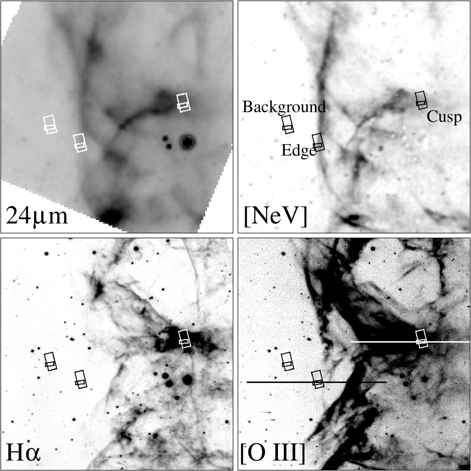
Figure 1: Images of the XA region, with IRS apertures overlaid. Left, top: Spitzer MIPS 24$\mu$m image, Right, top: [Ne V] $\lambda$3426 image, Left, bottom: H$\alpha$ image, and Right, bottom: [O III] image, stretched to show the faint emission. The boxes represent IRS apertures drawn to scale, Short-High $4.7\arcsec\times 11.3\arcsec$ and Long-High $11.1\arcsec\times 22.3\arcsec$. The positions are labeled on the [Ne V] image. The locations where long-slit spectra were obtained are shown on the [O III] image. (Note that the Western edge of the slit at the Cusp position extended beyond the image field of view.)

The MIPS 24 $\mu$m image of the XA region is shown in the top-left panel of Figure 1. Going clockwise, the remaining panels show [Ne V] $\lambda$3426, [O III] $\lambda$5007, and H$\alpha$ narrowband images obtained at the 1.2 m telescope at the Whipple Observatory, located on Mount Hopkins, Arizona. Overlaid on the images are boxes showing the locations of the IRS apertures. The smaller boxes represent the $4.7\arcsec\times 11.3\arcsec$ SH aperture and the larger boxes the $11.1\arcsec\times 22.3\arcsec$ LH aperture. The labels we use for the three positions, “Background”, “Edge”, and “Cusp” are shown on the [Ne V] image. Overlaid on the [O III] image are the locations of the slit positions through which optical spectra were obtained (in September 2012) using the 1.5 m Tillinghast telescope, also at the Whipple Observatory.

For the spectroscopic observations, we obtained the Basic Calibrated Data (BCD) and related “Level 1” files (AOR key 15087872) from the Spitzer archive. We used the “Spectroscopic Modeling Analysis and Reduction Tool” (SMART) version 8.1.2 (Higdon et al., 2004; Lebouteiller et al., 2010) to extract background-subtracted, one-dimensional, calibrated data. The observations of the Background region outside the remnant were used for background subtraction. In order to check for consistency, we used the Spitzer IRS Custom Extraction (SPICE) software to extract the spectra from the Cusp region. The extraction was performed on only one of the two nod positions. The background was subtracted, but there was no interactive removal of bad pixels. Due to the remaining bad pixels, the resulting spectra were noisier than the ones extracted using SMART, but the line positions and fluxes in the two spectra matched extremely well. In this paper, we use only the spectra that were extracted using SMART.

The long-slit optical spectra were obtained using the FAST spectrograph (Fabricant et al., 1998) through a 2″ wide slit. The slit length is about 3′ and the spatial axis was oriented in the E-W direction, and centered close to the Short-High aperture positions. The spectrophotometric standards BD+253941, BD+174708 and HD19445 were also observed, and used to calibrate the XA region data. The 2-D spectra have an angular scale of 0.57″/pixel and are binned by 2 pixels, and they have a wavelength scale of 1.472Å/pixel.

For the Cusp region, we also include an International Ultraviolet Explorer (IUE) spectrum reported by Danforth et al. (2001). Their position 1M coincides with the Spitzer SH position, although the 10″ by 20″ IUE aperture is much larger. We discuss the scaling of the fluxes in the different apertures below.

3 Results from the Infrared Spectra

The two positions selected for observation sample different shock interactions. The Edge is the shock at the outer perimeter of the remnant. The [Ne V] emission is strong, but the post-shock material has not yet recombined and therefore the H$\alpha$ emission is undetected (Figure 1). The Cusp is a region of complex morphology at the tip of a cloud protrusion, and both in [Ne V] and in H$\alpha$ emission line images.

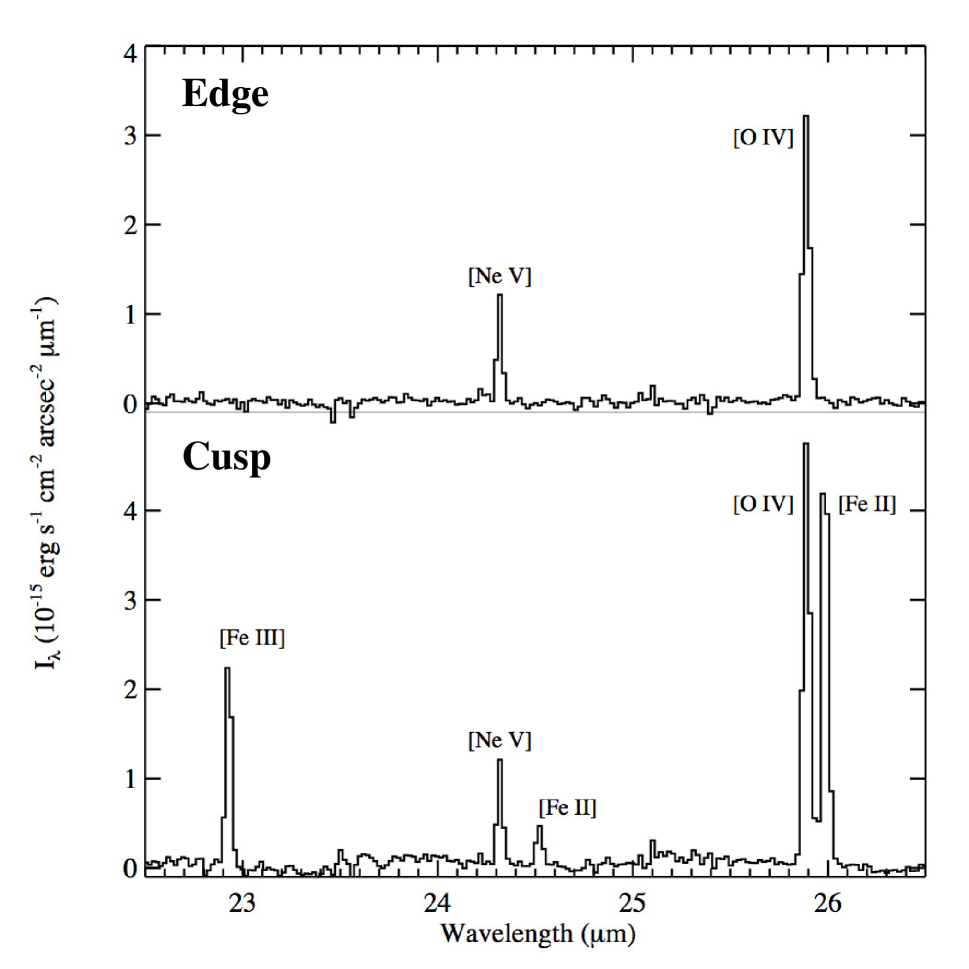
Figure 2: Background subtracted Long-High spectra of the Edge and Cusp shocks in the 22.5–26.5$\mu$m wavelength region. Note that [O IV] and [Fe II] lines are well resolved.

The Edge spectrum contains only [Ne V] and [O IV] lines, both of which are high ionization species. By contrast, the Cusp spectrum is rich in lines, and includes emission from high and low ionization species, such as [O IV], [Ne II], [Si II] and [Fe II]. Spectra in the 22.5–26.5 $\mu$m range are plotted for both locations in Figure 2, and the IR spectrum of the Cusp is shown in Figure 3.

The line strengths in each of the spectra were measured using both a simple integration under the curve and gaussian fitting; the two measurements are consistent to within the statistical errors, which we estimate to be about 5% for the strong lines and about 15% for the weak lines. In the Edge SH spectrum the intensity of [Ne V] 14.33 $\mu$m is $3.6\times 10^{-17}$ erg s^-1 cm^-2 arcsec^-2. In the LH spectrum, the intensity of [Ne V] 24.32 $\mu$m is $4.1\times 10^{-17}$ erg s^-1 cm^-2 arcsec^-2, and of [O IV] 25.88 $\mu$m is $14.0\times 10^{-17}$ erg s^-1 cm^-2 arcsec^-2.

The line intensities measured in the Cusp spectra are presented in Table 2 along with the UV line intensities from Danforth et al. (2001) and optical line fluxes from FAST. The values reported are from the gaussian fits.

The high resolution modes of the IRS are not optimal for detecting low-level continuum emission. In order to check for a possible contribution from the dust continuum, we compared the MIPS 24 $\mu$m image flux from each of the LH apertures (after subtracting the flux from the background aperture) with the fluxes from the IRS spectra convolved with the MIPS 24 $\mu$m filter response curve. We find that for both the Edge and the Cusp, the IRS value was about 80% of the MIPS value. The emission from the XA region is completely dominated by the collisionally excited lines, with at most 20% contribution from thermal dust.

4 Results from Optical Spectroscopy

4.1 [O III] Emission from the Edge

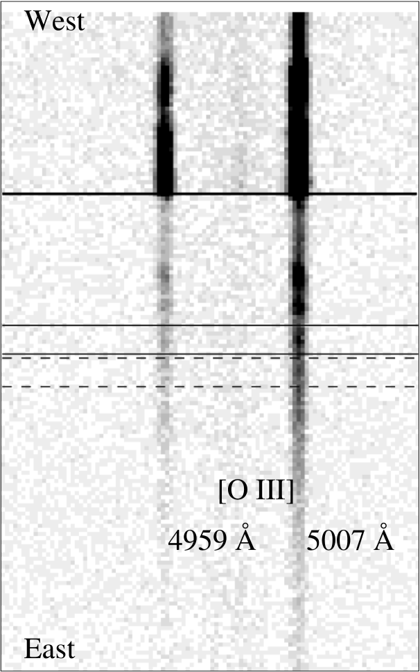
Figure 4: Two-dimensional long-slit spectrum across the Edge position showing the wavelength region around the [O III] $\lambda\lambda$4959,5007 doublet. The region corresponding to the Edge shock is shown between the two solid lines in the middle of the image. The region chosen for the background lies between the dashed lines. The thicker solid line indicates a position about 40″ towards the interior of the remnant demarcated by bright optical emission, evident in the [O III] image (Fig. 1).

Fig. 4 shows the 2-D spectrum of the slit lying across the Edge shock, in the wavelength region 4900–5050Å, which includes the [O III] doublet. The spatial axis is vertical, with East at the bottom and West at the top. The location of the Edge shock is between the pair of thin solid lines across the center of the image. The thick solid line about 3/4 the way up demarcates the boundary of the bright radiative filament, about 40″ West of the Edge shock. Faint [O III] emission extends beyond the location of the Edge shock. A few features corresponding to places where the slit crosses shock fronts are clearly seen. The Edge shock is easily identified, both because it is in the middle of the slit, and from its distance to the bright radiative shock, which is consistent with the separation seen in the [O III] image (Fig. 1).

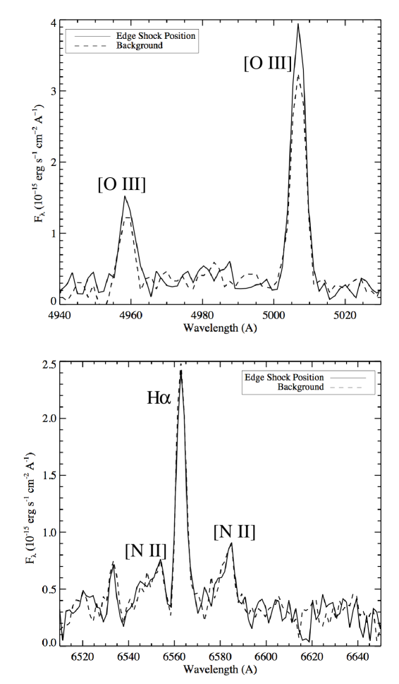
Figure 5: Flux-calibrated spectra of the Edge shock and of the background extracted from the regions shown in the 2D spectrum in Fig. 4. The top plot shows the [O III] lines, and the bottom plot shows the wavelength region around the H$\alpha$ and [N II] lines.

Spectra were extracted over 8 spatial pixels (9.12″) corresponding to the Edge shock position, and an adjacent region of the same width lying beyond the edge. These are shown by pairs of solid and dashed lines, respectively, on the image of the 2-D spectrum. The extracted, flux-calibrated spectra are shown in Fig. 5. The top plot shows the region around the [O III] lines, and the excess flux in the Edge shock position is clearly seen. The H$\alpha$ and [N II] are shown in the bottom plot - they are detected in both Edge and background spectra and of equal strengths. (The [S II] lines, not shown, are likewise detected at both positions with equal strengths.) We therefore ascribe the excess [O III] flux in the Edge shock position to emission from the shock itself, and the remaining as part of the background.

We obtained the fluxes in the [O III] $\lambda$5007 line in each of the spectra by fitting gaussians, and by integrating under the lines and subtracting the backgrounds. The methods yielded results within 3% of each other. We also found that the strength of the weaker line, [O III] $\lambda$4959 was 1/3 of the stronger line as expected.

The [O III] $\lambda$5007 fluxes are $1.84\times 10^{-14}$ erg s^-1 cm^-2 for the Edge position and $1.52\times 10^{-14}$ erg s^-1 cm^-2 for the background. The flux due to the Edge shock, which we take to be the difference between the two, is $3.2\times 10^{-15}$ erg s^-1 cm^-2 . Assuming that the emission fills the 2″ wide slit, and noting the angular region over which the spectrum was extracted, the observed [O III] $\lambda$5007 surface brightness of the Edge shock is $1.75\times 10^{-16}$ erg s^-1 cm^-2 arcsec^-2 .

4.2 Optical Spectrum of the Cusp

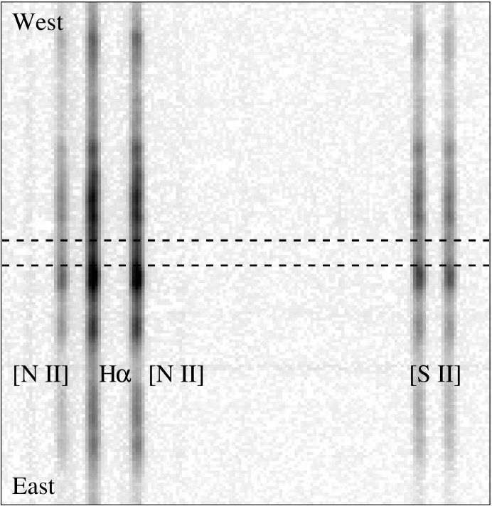
Figure 6: Two-dimensional long-slit spectrum across the Cusp position showing the wavelength region between 6520 Å and 6750 Å. The emission lines, [N II] $\lambda\lambda$6548,6584, H$\alpha$ $\lambda$6563 and [S II] $\lambda\lambda$6716,6731 are visible along the entire slit. The dashed lines demarcate the Cusp region targeted in the Spitzer spectra.

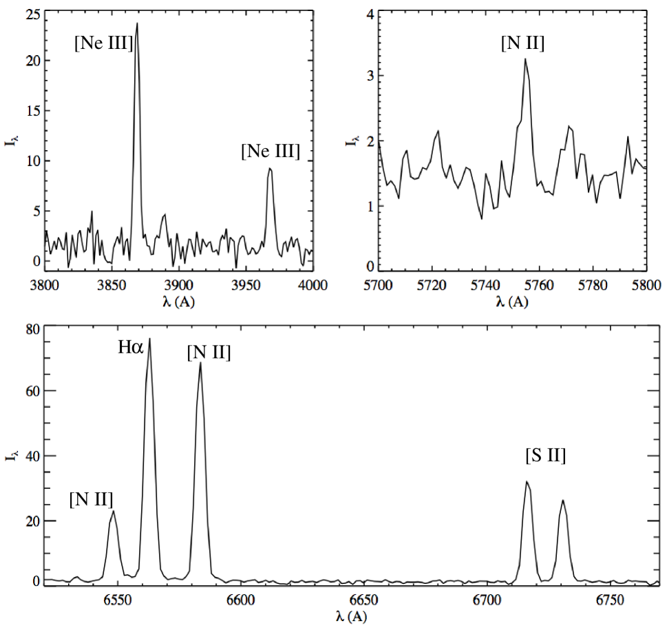
Figure 7: Selected wavelength regions of the Cusp spectrum, which was extracted along the region between the dashed lines shown in Fig. 6. The intensity units are $10^{-17}$ erg s^-1 cm^-2 arcsec^-2 Å^-1.

Fig. 6 shows the 2-D spectrum of the Cusp between 6520Å and 6750Å, which includes [N II], H$\alpha$ and [S II] lines (labeled on the image). The spatial axis is vertical with East at the bottom and West at the top. The region between the dashed lines in the figure is approximately that overlapping the IRS apertures. We extracted the 1-D spectrum from that region, 10.26″ wide, and measured the line fluxes, which are reported in Table 2. Selected regions of the spectrum, illustrating the range of line strengths measured, are plotted in Fig. 7. The statistical errors are $\leq 2$% for fluxes $\gtrsim 100\times 10^{-17}$ erg s^-1 cm^-2 arcsec^-2.

The Balmer decrement and the [O II] I₇₃₃₀/I₃₇₂₇ ratio from the optical spectrum of the Cusp indicate that E${}_{B-V}\sim 0.16$. The usual reddening assumed for the Cygnus Loop is E${}_{B-V}=0.08$, but Fesen, Blair & Kirshner (1982) have measured a range of Balmer decrements in optical spectra, and they suggest an additional 0.05–0.10 magnitudes of reddening towards certain filaments. In Table 2 we present the reddening corrected fluxes for E${}_{B-V}=0.16$.

In the Cusp spectrum, the ratio between the components of the [S II] doublet, F₆₇₁₆/F${}_{6731}=1.24\pm 0.03$. For temperatures in the range 5000–20,000 K, this implies electron densities in the range 100–250 cm^-3. (The calculations reported in this section were done using PyNeb Luridana, Morisset & Shaw (2012).)

[N II] $\lambda$5755 is detected in our Cusp spectrum at a level $\geq 3\sigma$ (Fig. 7). The temperature sensitive ratio I_[5755]/I_[6548+6584] equals $(10\pm 3)/429$ (Table 2), which implies that the temperature is about $14,200\pm\,2300$ K, consistent with the values used in the density calculation, above. The temperature-sensitive ratio [O III] I_[4363]/I_[5007+4949] is 0.08, which indicates that the [O III] emission arises at about 80,000 K, a much higher temperature than the typical average value of 25,000 K found in a complete radiative shock. That implies that the shock is incomplete, so that the swept-up column density is small enough that radiative cooling (Raymond et al., 1988) has only brought the temperature the gas shocked earliest to 7000 to 8000 K, and recombination is far from complete. This provides a constraint on the models, discussed below.

Fig. 6 shows that emission is detected across the entire slit, and variations in the line intensities are evident. In order to check how sensitive our results were to the exact region of extraction, we compared the Cusp spectrum with the spectrum of the brighter knot lying adjacent and to the East of the Cusp. The lines are brighter by a factor of $\sim$1.4 but the relative fluxes are approximately the same. In particular, the [S II], [N II] and [O III] density and temperature sensitive line-ratios are consistent within the error bars. Also, F${}_{{\rm{[S\,II]}}}$/F${}_{{\rm{H}}\alpha}\approx 0.8$ in both spectra.

5 Analysis and Discussion

For non-uniform extended emission observations with IRS the relative calibration of the SH and LH modules is highly uncertain (L. Armus, private communication). The absence of any continuum emission means that spectra from the two modules cannot be easily normalized. Additionally, since the SH aperture covers only about one-fifth the area of the LH aperture, the two sample different emitting regions. However, the ratio of the [Ne V] lines at 14.33$\mu$m and 24.32$\mu$m is determined solely by the excitation rates in the density and temperature range of interest, and we use that ratio to scale the fluxes (see below).

The shock models were calculated using the code originally described by Raymond (1979) with updates described in Raymond et al. (1997). We have further updated the code to use the recombination rates used by the CHIANTI package version 7.1 (Dere et al., 1997; Landi et al., 2013), which corrects errors in the rates for singly and doubly ionized species in version 6. We have also updated the collision strengths for the IR lines, many of which have strong contributions from resonances. The data used include Aggarwal & Keenan (2008) for [O IV], Witthoeft et al. (2007) for [Ne II], McLaughlin et al. (2011) for [Ne III], Dance et al. (2013) for [Ne V], Bautista et al. (2009) for [Si II], Grieve et al. (2013) for [S III] and Tayal (2000) for [S IV]. In addition, at the temperatures where O IV and Ne V are found in collisionally ionized plasmas, the contributions of excitation by proton collisions and of cascades from excitations to higher levels can be important. We used CHIANTI to include those effects. The [Fe II] line intensities were computed from the 52-level model of Bautista & Pradhan (1998), under the assumption of pure collisional excitation, and the [Fe III] line intensities were calculated using the 36-level model of Bautista, Ballance & Quinet (2010).

5.1 The Edge Shock

A far-ultraviolet spectrum of the Edge shock, obtained using FUSE, was analyzed by Sankrit et al. (2007). They found that the spectrum could be produced by a 180 km s^-1 shock and a swept-up column density $1.66\times 10^{18}$ cm^-2. At this stage of shock-completeness (swept-up column density at a given shock speed), the Ne⁴⁺ zone is nearly complete, while the O³⁺ zone is about 85% complete, and O²⁺ zone is just starting to develop. Thus the [O III] $\lambda$5007 to [O IV] ratio, which is independent of the oxygen abundance, is very sensitive to the swept-up column, while the [O IV] to [Ne V] flux ratio is less sensitive.

From §4.1 and §3, the observed [O III] to [O IV] flux ratio is 1.25. Corrected for interstellar extinction, using E_B-V=0.08 towards the Cygnus Loop (Parker, 1967), R${}_{V}=3.1$, and the prescription of Cardelli, Clayton & Mathis (1989) implemented in the IDL astronomy library of routines, the ratio is $\approx 1.6$. (Note that we have used E_B-V=0.16 for the Cusp region – this difference will be discussed further in §5.2, below.) The Edge shock does not fill the Long-High aperture, as is evident from the [Ne V] image shown in Fig. 1, and so the reported surface brightness is likely to be an underestimate. If we assume that the filling fraction is 0.5, then the resulting [O III] to [O IV] would be $\approx 0.8$.

In Fig. 8 the [O III] to [O IV] flux ratio is plotted as a function of swept-up column for a 180 km s^-1 shock. The dashed lines mark the two points bracketing the observed value – 0.8 and 1.6. At these points, for O=8.70 and Ne=8.09, the values of the [O IV] to [Ne V] flux ratio are 1.6 and 2.2, respectively. For a given shock velocity, and for a particular swept-up column this flux ratio is directly proportional to the abundance ratio, O/Ne. In the model, O/Ne = 4.1, and the observed value of [O IV] to [Ne V] is 3.4. Scaling the model to match the observed values at the two points, we find that the required values of O/Ne are 8.9 and 6.3 for the lower and higher swept-up columns.

The [Ne V] emissivity is sensitive to the shock velocity around the 180 km s^-1 region, with faster shocks producing brighter [Ne V] emission. The shock velocity is well constrained to be 180 km s^-1 by the Ne VI] to Ne V] ratio in the FUV spectrum (Sankrit et al., 2007). The observed Ne VI] emission would not be produced by slower shocks. Therefore, we performed the calculation described above only for a faster, 190 km s^-1, shock, and found that O/Ne in the range 9.1 to 13.2 are required.

Our choice of the oxygen to neon abundance ratio for the original model was based on its success in reproducing the FUV line strengths (Sankrit et al., 2007). However, updates to the atomic rates (see §5, above) have resulted in a revision of the ratio of abundances. Furthermore, the forbidden optical and IR lines are not susceptible to uncertainties due to resonance scattering, and therefore the results presented here are more robust than those from the earlier study. The abundance ratio O/Ne=6.3 is close to the median value of 5.89 found for a sample of 10 Galactic H II regions (Shaver et al., 1983). The maximum value of the ratio was 8.9 in the sample. Thus, the O/Ne we find for the 180 km s^-1 shock are in the normal range for H II regions, while the high values found for the 190 km s^-1 shock are implausible.

5.2 The Cusp Region

To compare the observations of the Cusp with theoretical models, we must apply a reddening correction and scale the fluxes from the different apertures to account for the variation in surface brightness within the larger apertures. The value for E_B-V obtained from the optical spectrum differs from the usual value for the Cygnus Loop (§4.2). As a check, we extracted the flux in the [Ne V] 3425 Å line in the region of the Spitzer SH aperture from the image presented by Szentgyorgyi et al. (2000) and compared it with the [Ne V] 14.33 $\mu$m flux, and the ratio agrees with the theoretical value and E${}_{B-V}=0.08$.

The difference in the values of E_B-V derived from the Balmer decrement and the [O II] lines on the one hand, and from the [Ne V] optical and IR lines on the other is consistent with the idea that on average the Balmer lines and low-ionization lines arise from deeper within the interaction region and the high-ionization lines from the outer, less extincted regions. The reddening, E${}_{B-V}=0.08$ is the normal foreground, and the excess is local. An extended component of high ionization emission has been observed in the XA region. FUSE spectra presented by Sankrit et al. (2007) shows the presence widespread O VI $\lambda\lambda$1032,1038 emission, and strong O VI emission, comparable in strength to the O IV] $\lambda$1400 line, was observed in the area by HUT (Danforth et al., 2001). These provide some evidence for a faster shock, or for a transition layer where cool gas evaporates to join the X-ray emitting plasma that envelopes the optical filaments. However, the 56″ HUT aperture encompasses a lot of material outside the region observed by the other instruments considered here, so there is no compelling evidence for a faster shock contributing specifically to the spectra we have observed. An alternative explanation of the discrepancy is that we have underestimated the error in the surface brightness measured from the narrowband image, both due to the calibration and due to the placement of the SH aperture FOV on the image, and the result is consistent with the higher value of reddening.

Faced with these possibly contradictory results, we calculated the corrected spectrum for both values of reddening, using the Cardelli, Clayton & Mathis (1989) extinction function with R${}_{V}=3.1$. After applying the reddening correction, we accounted for the large variations of intensity within the different apertures by scaling the fluxes to match theoretical intensity ratios. Ideally intensity ratios that depend only on the atomic rates, and are therefore insensitive to the model should be used. The ratio of the two IR lines of [Ne V] is one such ratio. To scale the LH aperture to the SH we use the [Ne V] 14.33 $\mu$m to 24.32 $\mu$m ratio=0.82. This means multiplying the LH values by a factor of 1.90, which is plausible because the average flux in the LH aperture is presumably lower than in the SH aperture, which was placed on the intensity peak as judged by the optical images. This scaling greatly improves the agreement of the [S III] 18.71 $\mu$m to 33.47 $\mu$m ratio. (We use the [Ne V] ratio rather then the [S III] ratio, because the latter depends on density in the range indicated by the [S II] optical lines.)

For the optical and UV fluxes, the only ratios available have some temperature sensitivity, so the scaling is less certain. To scale the optical flux to the SH flux we use the [Ne III] $\lambda\lambda$3870,3968 to 15.56 $\mu$m ratio of 3.87. Since that depends on the reddening correction, the scalings differ for the two reddenings chosen; 1.0 for E${}_{B-V}=0.08$ and 0.70 for E${}_{B-V}=0.16$. Next, we scale the UV fluxes by using the O III] 1665Å to [O III] 5007Å ratio of 0.52. That results in multiplying the UV fluxes by 1.90 for E${}_{B-V}=0.08$ and 1.0 for E${}_{B-V}=0.16$. The reddening-corrected [Ne V] $\lambda$3425 intensities were not scaled, because the flux was extracted from the region corresponding to the SH aperture. The uncertainty in the placement of the aperture on the image gives a 7% uncertainty, and Szentgyorgyi et al. (2000) quote a photometric uncertainty of 30%. Finally, we normalized the relative fluxes to H$\beta=100$, for comparison with the models.

The scaling for the different apertures largely cancels out the difference in reddening correction, so that for the two values of E_B-V, the scaled, normalized relative fluxes differed by less than 20% for all lines except [Ne V] $\lambda$3425. In Table 2 along with the observed fluxes, we present the reddening corrected fluxes only for the case of E${}_{B-V}=0.16$ because of its better agreement with the model Balmer decrement.

5.2.1 Shock Models

The line fluxes predicted by a set of shock models are presented in Table 2. We chose five models to illustrate the sensitivity to shock speed and density. These models use the following abundance set: H=12.00; He=10.93; C=8.52; N=7.96; O=8.70; Ne=8.09; Mg=7.52; Si=7.60; S=7.20; Ar=6.90; Ca=6.30; Fe=7.60 and Ni=6.30. Hydrogen was assumed ionized and the helium singly ionized in the pre-shock gas. The shock velocities, pre-shock densities and pre-shock magnetic fields used in these models are presented in Table 3, along with values of the swept-up column densities and temperatures where the models were truncated.

Shock Speed: The range of shock speeds 145–155 km s^-1 best reproduces the line fluxes from the wide range of ionization states that are observed. Shocks that are outside this velocity range produce far too little or far too much of high ionization lines such as N V, C IV, [O IV] and [Ne V] (although the permitted lines are so strongly attenuated by resonance scattering in the shocked gas and in the ISM that they only constrain the lower end of the range). The specific range was chosen to match the He II 1640 Å line under the assumption that Helium is singly ionized in the pre-shock medium.

Density and Magnetic Field: The observed ratio of $1.24\pm 0.03$ between the components of the [S II] doublet (§4.2) implies an electron density in the emitting gas in the range 100–250 cm^-3. The density in the [S II] zone depends upon the pre-shock density and on the maximum compression in the post-shock gas, which in turn depends on the driving pressure of the shock and on the pre-shock magnetic field and cosmic ray pressure. These non-thermal contributions to the pressure limit the compression of the gas as it cools from the post-shock temperature near 260,000 K to the [S II] formation temperature near 10,000 K (Raymond, 1979). The rather low values of the pre-shock magnetic field for most of the models were chosen in order to reach the observed density range with a pre-shock density and ram pressure comparable to those determined for other positions in the XA region. For the models shown, the predicted [S II] doublet ratio agrees with the observed value for M145, M150 and M155a. However, the predictions are too low for models M155b and M155c, indicating that the density is too high.

On the other hand, observed ratio of [Fe III] 22.92 $\mu$m to [Fe II] 25.98 $\mu$m is about 0.4, while the lower density models (M145, M150 and M155a) predict ratios of about 0.1. Even the higher density models (M155b and M155c) only predict ratios of 0.2, while their [S II] doublet ratios are clearly at odds with the observed value. The lower densities are consistent with those derived at other shocks in the Cygnus Loop, including several positions in the XA region, while the [Fe II] ratio would suggest a density of 2000 cm^-3, 10 to 20 times higher than found at other positions. The easiest explanation for the discrepancy is an error in atomic rates, but a physical explanation might be that the [Fe II] arises from a separate region, such as a slow shock that is heavily reddened and therefore contributes little to the [S II] lines.

Shock Completeness: The models in Table 2 are cut off at swept-up columns log $N_{H}$ = 18.0 to 18.1. The temperatures obtained at cut-off are between 7000 and 8000 K (Table 3), which is required by the temperature of the [O III] zone (§4.2). Although a somewhat larger range of cutoffs is allowable, too much of a deviation would lead to unacceptable values for line ratios such as [O II]/H$\beta$ and [O III]/H$\beta$. For the densities and magnetic fields used, the gas has cooled for between 500 and 1000 years. A 400 km s^-1 X-ray producing shock will travel ahead by the difference in velocities times that age, or about 100″ in a thousand years, which is consistent with the position of the Edge filament. The observed separation is 135″, which lies within the uncertainty in projection effects and the changing speeds of the shocks as they pass through regions of different density.

5.2.2 Comparing the IR spectra with Shock Models

The parameters in the shock model have been constrained largely by the UV and optical spectra. If we disregard the lines strongly affected by resonance scattering, and [Ne V] $\lambda$3425, for which the measurement and scaling is discrepant compared to the other lines, then the shock model predictions match the observations to within 50%, except for N III] $\lambda$1750 and [Ar III] $\lambda$7138, and in most cases to within 25%. Reducing the rather uncertain abundance of Ar by a factor of about two would bring the [Ar III] predictions into agreement with the observed value, without affecting any other line strengths.

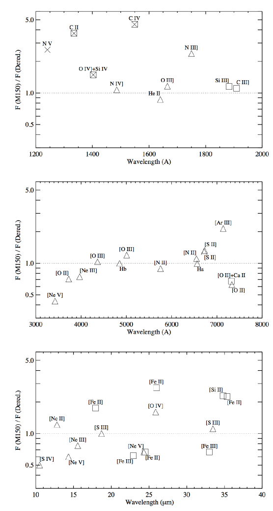
Figure 9: The ratio between the model M150 predicted flux and the observed (scaled, dereddened) value is plotted against wavelength for the lines listed in Table 2. In the case where the flux is a sum of two components, the first wavelength value reported in column 2 of the table is used in the plot. The top, middle and bottom plots show the UV, optical and IR lines, respectively. Squares indicate lines affected by depletion on to dust grains, and crosses indicate lines likely to be attenuated by resonance scattering. Crosses within squares are used for lines susceptible to both depletion and resonance scattering.

In Fig. 9, the ratio of the flux predicted by model M150 to the observed, dereddened value is plotted against wavelength for the lines listed in Table 2. The top, middle and bottom plots show the UV, optical and IR lines, respectively. It should be noted that no distinction is made between strong and weak lines in the plots. So, for instance, the match between models and observation for the weak [Fe III] lines in the IR spectrum is actually much better than the plot seems to imply, as can be seen by examining Table 2.

We now turn to an examination of the IR lines, focusing on models M145, M150 and M155a, since the other two (M155b and M155c) do not predict the observed optical [S II] doublet ratio. The [Ne V] lines are most sensitive to the shock velocity, and are best matched by the 155 km s^-1 shock. All models predict [O IV] fluxes that are higher than the observation – a factor of 1.3 for the 145 km s^-1 shock and 2.0 for the 155 km s^-1 shock. The models reproduce the correct [S III] line fluxes, with the 150 km s^-1 model providing the best match. In contrast, the models consistently predict only about half the observed [S IV] flux.

The [Si II] fluxes predicted by the model are significantly higher than the observed value. Reducing the Si abundance by a factor of about 2.5, as expected from depletion onto grains, would bring them into agreement. However, the line fluxes predicted by the models are also sensitive to the column density cut-off, since the [Si II] emission would extend far into the cooling zone.

The ratios among the [Fe II] lines predicted by the models are in agreement with the observed values, but the absolute fluxes are higher. As with silicon, the match between models and observation would be improved for the [Fe II] lines with Fe abundances reduced by a factor of about two. The models correctly predict the [Fe III] line fluxes, and therefore too low a ratio between [Fe III] and [Fe II] line strengths. The ratio is sensitive to the photoionization rate of Fe⁺, the recombination rate of Fe⁺⁺, and especially to the charge transfer rates, which we have taken from Neufeld & Dalgarno (1987) as well as to the cutoff column density.

The models assumed solar abundances for Si and Fe, while those elements should be almost entirely depleted onto dust grains in the ISM. Reductions by factors of 2.5 and 2, respectively, still imply that about 40–50% of these elements have been returned to the gas phase. The ratios of the UV lines of C III] and Si III] to the O III] line also indicate only modest depletion. This efficient liberation of refractory elements from grains is a little surprising, since only about 20–40% of the silicon and carbon are returned to the gas phase at a swept-up column of $2\times 10^{18}$ cm^-2 in the faster X-ray producing shock in the NE Cygnus Loop studied by Raymond et al. (2013). The sputtering rates are greatly reduced at the lower temperatures in 150 km s^-1 shocks, but grain-grain collisions shatter the dust particles, producing small grains that are more vulnerable to sputtering. Jones, Tielens, & Hollenbach (1996) find that 10% to 30% of the mass of graphite and silicates in grains is returned to the gas phase for shock speeds below 150 km s^-1, so the spectra imply a higher dust destruction efficiency. However, the behavior of grains in high speed collisions is uncertain.

The pair of lines [Ne II] and [Ne III] present an interesting puzzle, which may have some important consequences for our understanding of the XA region. Separately considered, the model predictions are in fairly good agreement with the observations. However, the [Ne III] to [Ne II] flux ratio is always less than 1. To match the predicted flux ratio of about 1.3, the models would need to be truncated at unacceptably low values of swept-up column density. The observed flux ratio can be explained if an additional source of photoionization is invoked. The extra photoionization would also be helpful in explaining the strength of the [S IV] line and possibly the [Fe III] to [Fe II] flux ratio as well.

5.2.3 Shock Driving Pressures

The driving pressures of the shocks M145, M150, M155a, M155b and M155c, n${}_{0}\times v_{shock}^{2}$, are $\approx$ $5.3\times 10^{4}$, $1.3\times 10^{5}$, $6.0\times 10^{4}$, $1.2\times 10^{5}$ and $1.9\times 10^{5}$ cm^-3 (km s^-1)², respectively. These values are 3 to 10 times higher than the driving pressure found for the Edge shock, $1.9\times 10^{4}$ cm^-3(km s^-1)², by Sankrit et al. (2007). The pressure derived is proportional to the pre-shock density, which in turn is proportional to the assumed distance to the Cygnus Loop. Sankrit et al. (2007) assumed 540 pc (Blair, Sankrit & Raymond, 2005), but the upper limit to the distance, 640 pc (Blair et al., 2009), or an even greater value, is supported by proper motion measurements of the non-radiative shocks in the NE Cygnus Loop (Salvesen, Raymond & Edgar, 2009). Furthermore, the reported errors on the density allow it to be about 30% higher. However, even if the driving pressure for the Edge shock is 2 times the value reported by Sankrit et al. (2007), that for the Cusp is higher by a factor between 1.5 and 5.

This may not be a problem since some pressure variations within the XA region due to the interaction of dense clouds are likely. We note that if the cosmic ray population in the Galaxy were simply compressed in the shock, it could provide a substantial fraction of the pressure support in the [S II] emitting region for densities (and therefore compression ratios) at the upper end of the range allowed by the [S II] line ratio. However, that assumes that the cosmic rays do not diffuse away during the cooling process.

5.2.4 Model Limitations

The comparison of the Cusp spectrum, from 1240 Å to 35 $\mu$m with models of radiative shocks, shown in Table 2 illustrates both the usefulness of the models and their limitations. There are many ways in which the models can be wrong. They assume steady flow as the gas cools until it reaches a sharp cutoff column density. That assumption can be violated by thermal instability in the cooling region (Innes, 1992), but that instability becomes strong at speeds above 150 km s^-1, and it takes more than one cooling time to develop. It is also violated if the density, and therefore shock speed, varies significantly over the distance in which the shock sweeps up the observed column, in this case about 0.1 pc, and that is very likely at the edge of a cloud. In that case the derived shock speed, which is determined by the highest ionization states observed, is near the current shock speed, while lower ionization species may have passed through a faster shock earlier in its evolution.

Other weaknesses of the simple model include the possibility of mixing with the high temperature gas that produces X-rays, the possible effects of thermal conduction, the neglect of dust and the gradual liberation of refractory elements, the uncertainties in atomic rates and the approximate treatment of radiative transfer. Weaknesses in the comparison to observations include the reddening correction uncertainty, and the scaling for the different apertures of the different instruments. We note that a single shock model could not be expected to match all the line intensities even if the apertures used in the different observations covered exactly the same area on the sky, because the echelle spectrum shown by Danforth et al. (2001) shows that there are two separate shocks along the line of sight, redshifted and blueshifted by about 30 km s^-1.

In spite of all the limitations described above, a simple model of a 145–155 km s^-1 shock is a reasonable explanation for the observations, since it matches all the observed lines to within a factor of 2 (except N III], where the discrepancy is slightly higher) and most to within about 25%. Although the match between observations and model predictions is reasonable, the agreement could be improved with some tweaking of model parameters, particularly elemental abundances and cutoff column densities. However, the parameter changes would probably lie within the uncertainties. The fact that such a simple model comes close to matching the observations may result from the fact that to first order it is simply conservation of energy in gas that cools radiatively from the shock temperature.

5.3 Comparison with other SNRs

The set of IR lines detected in the Cusp spectra are useful diagnostics of SNR shocks. This is particularly true of the lines from the singly and doubly ionized species, [Ne II], [Si II], [Fe II], [Ne III], [S III]and [Fe III], all of which can be produced in shocks with speeds as low as 80 km s^-1 (Hartigan, Raymond & Hartmann, 1987). We compare the IR line fluxes from the Cusp region with those measured in other SNRs. In Table Spitzer IRS Observations of the XA Region in the Cygnus Loop Supernova Remnant we have assembled measurements from the published literature. Our sample consists of Infrared Space Observatory spectra of IC443 (Oliva et al., 1999a) and RCW 103 (Oliva et al., 1999b), and Spitzer spectra of W44, W28, IC443C and 3C391 (Neufeld et al., 2007) and Kes 69, 3C396, Kes 17, G346.6-0.2, G348.5-0.0 and G349.7+0.2 (Hewitt et al., 2009).

The strongest lines in all the remnants are [Si II] 34.80 $\mu$m and [Ne II] 12.81$\mu$m. In Table Spitzer IRS Observations of the XA Region in the Cygnus Loop Supernova Remnant we have arranged the remnants in order of increasing surface brightness of the sum of these two lines. According to this measure, the Cygnus Loop XA region is the faintest of the sample. The remaining objects fall into three groups: at the faint end IC443C and G346.6-0.2 are about 3 times as bright as XA, the brightest remnants, RCW 103 and G349.7+0.2 are 70 and 180 times as bright as XA, respectively, and the remaining eight objects are between 7 and 30 times as bright.

The ratio of [Ne III] 15.56 $\mu$m to [Ne II] 12.81 $\mu$m in the XA region is 1.3, which is the highest value among all the remnants. The ratio is 1.2 in 3C396, 0.9 in RCW 103, and lies between 0.1 and 0.5 for all other remnants. Shocks with velocities in the 80–120 km s^-1 range produce [Ne III] to [Ne II] ratios between 0.1 and 0.3 when the pre-shock medium is in photoionization equilibrium, and between 0.5 and 0.9 when it is completely ionized (Hartigan, Raymond & Hartmann, 1987). We have explained the higher than predicted ratio in the Cusp spectrum by invoking an incomplete, $\sim 150$ km s^-1 shock. However, an alternative explanation is that faster shocks in the vicinity as well as the hot X-ray emitting plasma provide photoionizing radiation that increases the [Ne III] to [Ne II] flux ratio above the values expected for only shock excitation.

The [Fe III] 22.92 $\mu$m to [Fe II] 17.93 $\mu$m ratio is another potential diagnostic of the ionization state, though it can also depend on the density. (We do not use the [Fe II] 25.98 $\mu$m flux in the comparison since for the other remnants this line is not well resolved from the [O IV] 25.88 $\mu$m line.) The ratio of the intensities in the dereddened and scaled Cusp spectrum is 1.60, and in the uncorrected observed spectrum it is 0.91 (Table 2) The [Fe III] line is detected in four other remnants, RCW 103, W44, W28, and 3C391, and an upper limit is presented for IC443C. The [Fe III] to [Fe II] flux ratio ranges between 0.16 and 0.25, significantly lower than in the Cusp, and consistent with recombined shocks.

The [Ne III] and [S III] zones in the post-shock flow are nearly co-extensive and therefore the relative abundances of Ne and S influence the flux ratio of [Ne III] 15.56 $\mu$m and [S III] 18.71 $\mu$m. The ionization potential of S⁺⁺ (34.83 eV) is lower than that of Ne⁺ (40.96 eV) and therefore photoionization can also play a role in determining the flux ratio of [Ne III] to [S III]. This trend is detected in the sample of remnants. For the three objects with the lowest [Ne III] to [Ne II] ratios, i.e. $<0.16$, the [Ne III] to [S III] ratios lie between 0.5 and 1.4. For all the remaining objects, except one, where the [Ne III] to [Ne II] ratio span the range 0.2–1.3, the [Ne III] to [S III] ratios lie between 2.4 and 4.4. The exception is Kes 69, where the ratio is 8.2, indicating a higher Ne to S abundance in this remnant compared with the others.

The [S IV] line is detected in the XA region and in RCW 103, and in none of the other remnants. In RCW 103, the ratio [S IV] 10.51 $\mu$m to [S III] 18.71 $\mu$m is about 0.06, which is much lower than for the XA region, where the ratio is about 0.4. Overall, we conclude that the other spectra listed in Table 4 pertain to slower shocks, than the one at the Cusp, probably because the bright regions chosen for observation are shocks in denser clouds.

6 Concluding Remarks

The Cygnus Loop XA region provides a rich set of shock excited emission lines across a broad wavelength range. The analysis of the morphologically simple Edge shock can be accomplished with one-dimensional shock models. The emission line spectrum of the more complex interior Cusp shock can be reproduced approximately by a similar simple shock model. However, the limitations of the models imply a corresponding limitation in our interpretation of the shock interaction.

The proximity of the Cygnus Loop allows us to study the IR diagnostics of a radiative shock in detail. Our analysis of the XA emission lines will help in establishing robust diagnostics that can be applied to other SNRs, where, presumably, the IR spectra are obtained from regions even more heterogeneous and complex than the Cusp region.

Our data shows the lack of dust emission in the mid-IR wavelength range. Even the slower shocks are presumably effective at destroying the smaller grains likely to contribute at these wavelengths. To probe the dust and possible molecular content of the XA region, we will need observations at longer wavelengths. The complex morphology of the cloud shock interaction will be accompanied by comparably complicated kinematics. The identification and use of a kinematic tracer to map the velocity field in the XA region may be useful in disentangling the various shock components contributing to the emission.

By combining the IR spectrum of the Cusp with optical and UV spectra, we have obtained tight constraints on the shock speed, pre-shock density, elemental abundances and the column density cutoff, which corresponds to the age of the shock. We find that a speed of about 150 km s^-1 is needed to match the high ionization lines, rather efficient destruction of grains is required to match the abundances of refractory elements, and an age of about 1000 years matches the column density cut-off and separation between the Cusp and Edge regions.

Table 1: Summary of IRS observations

Label	$\alpha_{J2000}$	$\delta_{J2000}$	texp (SH)	texp (LH)
Cusp	$20^{\rm{h}}57^{\rm{m}}14\fs 82$	+31° 02′ 33$\farcs$4	481.7 s	241.8 s
Edge	$20^{\rm{h}}57^{\rm{m}}25\fs 42$	+31° 01′ 40$\farcs$5	481.7 s	241.8 s
Background	$20^{\rm{h}}57^{\rm{m}}28\fs 50$	+31° 02′ 04$\farcs$5	481.7 s	241.8 s

Table 2: Cusp Region: Observed and Model Fluxes

Ion	$\lambda$	Obs.	Dered.	M145	M150	M155a	M155b	M155c
Ultraviolet Lines
N V	1241	85	315	391	814	1230	1110	1050
C II	1335	33	103	456	382	481	448	433
O IV] +Si IV	1403	162	468	540	697	859	775	736
N IV]	1486	92	248	226	266	280	253	239
C IV	1549	183	476	2370	2150	2040	1800	1710
He II	1640	115	290	236	251	269	241	229
O III]	1665	145	363	378	421	492	446	425
N III]	1750	31	77	173	183	195	177	169
Si III]	1883	81	209	235	241	297	276	265
C III]	1909	232	611	701	675	801	731	698
Optical Lines
[Ne V]	3425	37	62	15	27	44	39	38
[O II]	3727	1298	1432	957	1012	1166	1073	1009
[Ne III]	3968+3870	165	176	120	131	152	139	134
[O III]	4363	59	60	56	62	72	65	62
H$\beta$	4850	105	100	100	100	100	100	100
[O III]	5007+4959	773	720	771	860	977	883	840
[N II]	5755	10	9	7	8	9	8	8
[N II]	6548+6584	429	345	349	382	380	378	379
H$\alpha$	6563	363	292	290	290	290	290	290
[S II]	6717	153	122	173	157	174	159	144
[S II]	6727	124	99	139	131	142	153	160
[Ar III]	7138	18	14	27	30	33	30	29
[O II] +Ca II	7320	64	49	34	33	39	41	38
[O II]	7330	42	32	19	20	24	25	26
Infrared Lines: Short-High Module
[S IV]	10.51	9.8	8	3	4	4	3	3
[Ne II]	12.81	46.9	37	50	45	43	47	49
[Ne V]	14.33	6.1	5	2	3	5	5	5
[Ne III]	15.56	59.5	47	30	36	35	30	29
[Fe II]	17.93	9.6	8	14	14	14	16	18
[S III]	18.71	24.3	19	16	19	14	14	14
Infrared Lines: Long-High Module
[Fe III]	22.92	8.7	13	8	8	11	9	9
[Ne V]	24.32	3.9	6	2	4	7	6	6
[Fe II]	24.51	1.9	3	2	2	2	3	3
[O IV]	25.88	21.7	33	42	53	65	58	55
[Fe II]	25.98	20.2	30	82	82	75	69	62
[Fe III]	33.00	2.2	3	2	2	3	2	2
[S III]	33.47	18.2	27	25	30	23	19	16
[Si II]	34.80	61.9	93	255	213	207	152	113
[Fe II]	35.34	5.1	8	18	18	16	15	14

Table 3: Shock Model Parameters

	M145	M150	M155a	M155b	M155c
Input Parameters
$v_{shock}$(km s-1)	145	150	155	155	155
n0(cm-3)	2.5	5.0	2.5	5.0	7.9
B0($\mu$G)	1.0	3.0	1.0	1.0	1.0
Value at Cutoff
log N(H)/(cm-2)	18.0	18.1	18.0	18.0	18.0
T(K)	7300	7700	7400	7300	7500

Note. — H ionized, He singly ionized in the pre-shock gas for all models.

Table 4: Selected IR flux and flux ratios of SNRs

SNR	[Ne II]+[Si II]	[Ne III]/[Ne II]	[Ne III]/[S III]	Ref.
CygLoop	110	1.27	2.4	1
IC443C	270	0.27	3.0	4
G346.6-0.2	290	0.07	1.4	5
W44	720	0.11	0.5	4
Kes 17	1090	0.35	4.4	5
3C396	1110	1.24	3.5	5
Kes 69	1150	0.24	8.2	5
IC443	1260	0.56	2.5	2
W28	1560	0.16	1.0	4
G348.5-0.0	3120	0.20	4.2	5
3C391	3230	0.38	2.6	4
RCW 103	7420	0.89	3.1	3
G349.7+0.2	19620	0.34	3.8	5

Note. — The lines reported are [Ne II] 12.81 $\mu$m, [Ne III] 15.56 $\mu$m, [S III] 18.71 $\mu$m and [Si II] 34.80 $\mu$m.

References. — 1. this work, 2. Oliva et al. 1999a, 3. Oliva et al. 1999b, 4. Neufeld et al. 2007, 5. Hewitt et al. 2009

Figure 3: IRS short-high (upper panel) and long-high (lower panel) spectra of the Cusp. The region between 19.5 $\mu$m and 22.5 $\mu$m contains no emission lines, and is not shown. Most of the low level spikes – positive and negative – are artefacts.

Figure 8: The plot shows the flux ratio between [O III] $\lambda$5007 and [O IV] 25.88$\mu$m as a function of swept-up column density for the fiducial model. The dashed lines indicate the points where the prediction matches the lower and upper bounds of the observed ratio. See §5.1 for details.

References

- Aggarwal & Keenan (2008) Aggarwal, K. M. & Keenan, F. P. 2008, A&A, 486, 1053.
- Arendt (1989) Arendt, R. G. 1989, ApJS, 70, 181.
- Arendt, Dwek & Leisawitz (1992) Arendt, R. G., Dwek, E., & Leisawitz, D. 1992, ApJ, 400, 562.
- Bautista & Pradhan (1998) Bautista, M. A., & Pradhan, A. K. 1998, ApJ, 492, 650.
- Bautista et al. (2009) Bautista, M. A., Quintet, P., Palmieri, P., Badnell, N. R., Dunn, J. & Arav, N. 2009, A&A. 508, 1527.
- Bautista, Ballance & Quinet (2010) Bautista, M. A., Ballance, C. P., & Quinet, P. 2010, ApJ, 718, L189.
- Blair, Sankrit & Raymond (2005) Blair, W. P., Sankrit, R., & Raymond, J. C. 2005, AJ, 129, 2268.
- Blair et al. (2009) Blair, W. P., Sankrit, R., Torres, S. I., Chayer, P., & Danforth, C. W. 2009, ApJ, 692, 335.
- Braun & Strom (1986) Braun, R., & Strom, R. G. 1986, A&A, 164, 208.
- Cardelli, Clayton & Mathis (1989) Cardelli, J. A., Clayton, G. C., & Mathis, J. S. 1989, ApJ, 345, 245.
- Dance et al. (2013) Dance, M., Palay, E., Nahar, S. N. & Pradhan, A. K. 2013, MNRAS, 435, 1576.
- Danforth et al. (2001) Danforth, C. W., Blair, W. P., & Raymond, J. C. 2001, AJ, 122, 938.
- Dere et al. (1997) Dere, K. P., Landi, E., Mason, H. E., Monsignori-Fossi, B. C. & Young, P. R. 1997, A&AS, 125, 149.
- Fabricant et al. (1998) Fabricant, D., Cheimets, P., Caldwell, N., & Geary, J. 1998, PASP, 110, 79.
- Fesen, Blair & Kirshner (1982) Fesen, R. A., Blair, W. P., & Kirshner, R. P. 1982, ApJ, 262, 171.
- Ghavamian et al. (2009) Ghavamian, P., Raymond, J. C., Blair, W. P., Long, K. S., Tappe, A., Park, S., & Winkler, P. F. 2009, ApJ, 696, 1307.
- Grieve et al. (2013) Grieve, M. F. R., Ramsbottom, C. A., Hudson, C. E. & Keenan, F. P. 2013, astroph-1308.1970.
- Hartigan, Raymond & Hartmann (1987) Hartigan, P., Raymond, J. C., & Hartmann, L. 1987, ApJ, 316, 323.
- Hester & Cox (1986) Hester, J. J., & Cox, D. P. 1986, ApJ, 300, 675.
- Hewitt et al. (2009) Hewitt, J. W., Rho, J., Andersen, M., & Reach, W. T. 2009, ApJ, 694, 1266.
- Higdon et al. (2004) Higdon, S. J. U., et al. 2004, PASP, 116, 975.
- Houck et al. (2004) Houck, J. R. et al. 2004, ApJS, 154, 18.
- Innes (1992) Innes, D. E. 1992, A&A, 256, 660.
- Jones, Tielens, & Hollenbach (1996) Jones, A. P., Tielens, A. G. G. M., & Hollenbach, D. J. 1996, ApJ, 469, 740.
- Landi et al. (2013) Landi, E., Young, P. R., Dere, K. P., Del Zanna, G. & Mason, H. E. 2013, ApJ, 763, 86.
- Lebouteiller et al. (2010) Lebouteiller, V., Bernard-Salas, J., Sloan, G. C., & Barry, D. J. 2010, PASP, 122, 231.
- Luridana, Morisset & Shaw (2012) Luridana, V., Morisset, C., & Shaw, R. A. 2012, IAU Symposium, 283, 422.
- McLaughlin et al. (2011) McLaughlin, B. M., Lee, T.-G., Ludlow, J. A., Landi, E., Loch, S. D., Pindzola, M. S. & Ballance, C. P. 2011, JPB, 44, 5206.
- Neufeld & Dalgarno (1987) Neufeld, D.A. & Dalgarno, A. 1987, PhRvA, 35, 3142.
- Neufeld et al. (2007) Neufeld, D. A., Hollenbach, D. J., Kaufman, M. J., Snell, R. L., Melnick, G. J., Bergin, E. A., & Sonnentrucker, P. 2007, ApJ, 664, 890.
- Oliva et al. (1999a) Oliva, E., Lutz, D., Drapatz, S., & Moorwood, A. F. M. 1999, A&A, 341, L75.
- Oliva et al. (1999b) Oliva, E., Moorwood, A. F. M., Drapatz, S., Lutz, D., & Sturm, E. 1999, A&A, 343, 943.
- Parker (1967) Parker, R. A. R. 1967, ApJ, 149, 363.
- Raymond (1979) Raymond, J. C. 1979, ApJS, 39, 1.
- Raymond et al. (1988) Raymond, J. C., Hester, J. J., Cox, D., Blair, W. P., Fesen, R. A. & Gull, T. R. 1988, ApJ, 324, 869.
- Raymond et al. (1997) Raymond, J. C., Blair, W. P., Long, K. S., Vancura, O., Edgar, R. J., Morse, J., Hartigan, P., & Sanders, W. T. 1997, ApJ, 482, 881.
- Raymond et al. (2013) Raymond, J. C., Ghavamian, P., Williams, B.J., Blair, W.P., Borkowski, K.J., Gaetz, T. J., & Sankrit, R. 2013, ApJ, 778, 161.
- Rho et al. (2009) Rho, J., Reach, W. T., Tappe, A., Hwang, U., Slavin, J. D., Kozasa, T., & Dunne, L. 2009, ApJ, 700, 579.
- Saken, Fesen & Shull (1992) Saken, J. M., Fesen, R. A., & Shull, J. M. 1992, ApJS, 81, 715.
- Salvesen, Raymond & Edgar (2009) Salvesen, G., Raymond, J. C., & Edgar, R. J. 2009. ApJ, 702, 327.
- Sankrit et al. (2007) Sankrit, R., Blair, W. P., Cheng, J. Y., Raymond, J. C., Gaetz, T. J., & Szentgyorgyi, A. 2007, AJ, 133, 1383.
- Sankrit et al. (2010) Sankrit, R., Williams, B. J., Borkowski, K. J., Gaetz, T. J., Raymond, J. C., Blair,W. P., Ghavamian, P., Long, K. S. & Reynolds, S. P. 2010, ApJ, 712, 1092.
- Shaver et al. (1983) Shaver, P. A., McGee, R. X., Newton, L. M., Danks, A. C., & Pottasch, S. R. 1983, MNRAS, 204, 53.
- Szentgyorgyi et al. (2000) Szentgyorgyi, A. H., Raymond, J. C., Hester, J. J., & Curiel, S. 2000, ApJ, 529, 279.
- Tayal (2000) Tayal, S. S. 2000, ApJ, 530, 1091.
- Temim et al. (2006) Temim, T. et al. 2006, AJ, 132, 1610.
- Temim et al. (2010) Temim, T., et al. 2010, ApJ, 710, 309.
- Winkler et al. (2013) Winkler, P. F., et al. 2013, ApJ, 764, 156.
- Witthoeft et al. (2007) Witthoeft, M. C., Whiteford, A. D. & Badnell, N. R. 2007, JPB, 40, 2969.