A time-splitting finite-element approximation for the Ericksen-Leslie equations

Abstract

In this paper we propose a time-splitting finite-element scheme for approximating solutions of the Ericksen-Leslie equations governing the flow of nematic liquid crystals. These equations are to be solved for a velocity vector field and a scalar pressure as well as a director vector field representing the direction along which the molecules of the liquid crystal are oriented.

The algorithm is designed at two levels. First, at the variational level, the velocity, pressure and director are computed separately, but the director field has to be computed together with an auxiliary variable in order to deduce a priori energy estimates. Second, at the algebraic level, one can avoid computing such an auxiliary variable if this is approximated by a piecewise constant finite-element space. Therefore, these two steps give rise to a numerical algorithm that computes separately only the primary variables. Moreover, we will use a pressure stabilization technique that allows an stable equal-order interpolation for the velocity and the pressure. Finally, some numerical simulations are performed in order to show the robustness and efficiency of the proposed numerical scheme and its accuracy.

Mathematics Subject Classification:Nematic liquid crystal; Finite elements; Projection method; Time-splitting method.

Keywords: 35Q35, 65M60, 76A15

1 Introduction

There has been a great interest in the finite-element numerical approximation of liquid crystal flows in recent years. The reason for this is that liquid crystals are not easy to be studied from experimental observations due to the effect of boundary conditions of the confining geometries. Thus, numerical simulations allow a clear insight into the behavior of liquid crystals and the understanding of their underlying physical properties. For instance, numerical simulations contribute to improve the design of practical devices.

Liquid crystals are materials that show intermediate transitions between a solid and a liquid called mesophases. It means that liquid crystals combine properties of both an isotropic liquid and a crystalline solid. These mesophases are due, in part, to the fact that liquid crystals are made of macromolecules of similar size, which are commonly represented like rods or plates. It is also known that the shape of the molecules play an important role in such mesophases. Moreover, liquid crystals depend on the temperature (thermotropic) and/or the concentration of a solute in a solvent (lyotropic) so that they can change from liquid to solid by means of varying the temperature and/or the concentration.

The mathematical theory describes liquid crystals attending to the different degrees of positional or orientational ordering of their molecules. Thus, the positional order alludes to the position of the molecules while the orientation order referred to the fact that the molecules to tend to be locally aligned towards certain preferred direction. Such a direction is described by a unit vector along the molecule if rod-shaped or perpendicular to the molecule if plate-shaped measuring the mean values of alignments.

The simplest phase of liquid crystals is called nematic which possesses an orientational ordering but not positional. That is, the molecules flow freely as in a disordered isotropic liquid phase while tend to be orientated along a direction which can be manipulated with mechanical (boundary conditions), magnetic or electric forces.

The simplest phenomenological description of spatial configurations in nematic liquid crystals is the Oseen-Frank theory [33, 16]. This approach consists in modeling equilibrium states as minima of a free-energy functional which is set up through symmetry and invariance principles, to capture some properties observed from experiments. Thus, the Oseen-Frank free energy is considered as a functional of the director vector ${\boldsymbol{d}}$. In its most basic form, the free energy functional is given by

$$E({\boldsymbol{d}})=\int_{\Omega}\left\{K_{1}|\nabla\cdot\nabla{\boldsymbol{d}}|^{2}+K_{2}({\boldsymbol{d}}\cdot(\nabla\times{\boldsymbol{d}}))^{2}+K_{3}({\boldsymbol{d}}\times(\nabla\times{\boldsymbol{d}}))^{2}\right\},$$

where $K_{1}$, $K_{2}$, and $K_{3}$ are the splay, twist, and bend elastic constants, respectively. Note that when these constants are equal, the Dirichlet energy becomes

$$E({\boldsymbol{d}})=K\int_{\Omega}|\nabla{\boldsymbol{d}}|^{2}.$$

Upon minimizing this energy subject to the sphere constraint $|{\boldsymbol{d}}|=1$, the following optimality system appears

$$-\Delta{\boldsymbol{d}}-|\nabla{\boldsymbol{d}}|^{2}{\boldsymbol{d}}=\boldsymbol{0}\quad\mbox{ in }\quad\Omega.$$

The limitation of the Oseen-Frank theory relies on the fact that it can only explain point defects in liquid crystal materials but not the more complicated line and surface defects that are also observed experimentally. The defect points or singularities in liquid crystals are regions where the anisotropic properties of molecules are broken. That is, the liquid crystal behaves as an isotropic fluid. Therefore, the director field cannot be defined. Mathematically, they are modeled by $|{\boldsymbol{d}}|=0$. One way of inducing defect points is with the help of the boundaries conditions.

The motion of defect points in liquid crystals can be studied via the long-time behavior of the harmonic map flow for which it is also interesting to incorporate the influence of the velocity. On the contrary, in many situations, the anisotropic local orientation of the director field influences the stress tensors that govern the fluid velocity. The hydrodynamic theory of nematic liquid crystals was established by Ericksen [14, 13] and Leslie [23, 24]. The fundamental system consists of a set of fully coupled, macroscopic equations, that contains the Oseen-Frank elastic theory governing the steady state, equilibrium solutions.

The remaining part of this paper is organized as follows. Section 2 starts by establishing some notation used throughout this paper. Then we follow with the differential formulation of the Ericksen-Leslie and the Ginzburg-Landau equations. To end the section, we sum up the main contributions on the finite-element approximation of the Ginzburg-Landau equations. In Section 3 we give some short-hand notation for finite-element spaces in order to be able to define the projection time-stepping algorithm and give a brief introduction to some key ideas leading to the proposed method. Next, in Section 4, we prove a priori estimates for the algorithm. Section 5 is devoted to some implementation improvements. Finally, we validate the numerical scheme with some simulations.

2 Statement of the problem

Let $\Omega\subset{\rm I}\hskip-2.41849pt{\rm R}^{M},M=2,3$ be any bounded open set with boundary $\partial\Omega$. For $1\leq p\leq\infty$, $L^{p}(\Omega)$ denote the space of $p$th-power integrable real-valued functions defined on $\Omega$ for the Lebesgue measure. This space is a Banach space endowed with the norm $\|v\|_{L^{p}(\Omega)}=(\int_{\Omega}|v({\boldsymbol{x}})|^{p}\,{\rm d}{\boldsymbol{x}})^{1/p}$ for $1\leq p<\infty$ or $\|v\|_{L^{\infty}(\Omega)}={\rm ess}\sup_{{\boldsymbol{x}}\in\Omega}|v({\boldsymbol{x}})|$ for $p=\infty$. In particular, $L^{2}(\Omega)$ is a Hilbert space with the inner product

$$\left(u,v\right)=\int_{\Omega}u({\boldsymbol{x}})v({\boldsymbol{x}}){\rm d}{\boldsymbol{x}},$$

and its norm is simply denoted by $\|\cdot\|$. For $m$ a non-negative integer, we define the classical Sobolev spaces as

$$H^{m}(\Omega)=\{v\in L^{p}(\Omega)\,;\,\partial^{k}v\in L^{p}(\Omega)\ \forall~{}|k|\leq m\},$$

associated to the norm

$$\|v\|_{H^{m}(\Omega)}=\left[\sum_{0\leq|k|\leq m}\|\partial^{k}v\|^{2}\right]^{\frac{1}{2}}\,,$$

where $k=(k_{1},\ldots,k_{M})\in{\mathds{N}^{M}}$ is a multi-index and $|k|=\sum_{i=1}^{M}k_{i}$, which is a Hilbert space with the obvious inner product. We will use boldfaced letters for spaces of vector functions and their elements, e.g. ${\boldsymbol{L}}^{2}(\Omega)$ in place of $L^{2}(\Omega)^{M}$.

Let $\mathcal{D}(\Omega)$ be the space of infinitely times differentiable functions with compact support on $\Omega$. The closure of ${\cal D}(\Omega)$ in $H^{m}(\Omega)$ is denoted by $H^{m}_{0}(\Omega)$. We will also make use of the following space of vector fields:

$$\boldsymbol{\mathcal{V}}=\{{\boldsymbol{v}}\in\boldsymbol{\mathcal{D}}(\Omega):\nabla\cdot{\boldsymbol{v}}=0\mbox{ in }\Omega\}.$$

We denote by ${\boldsymbol{H}}$ and ${\boldsymbol{V}}$, the closures of $\boldsymbol{\mathcal{V}}$, in the ${\boldsymbol{L}}^{2}(\Omega)$- and ${\boldsymbol{H}}^{1}(\Omega)$-norm, respectively, which are characterized by (see [38])

$${\boldsymbol{H}} = \{{\boldsymbol{u}}\in{\boldsymbol{L}}^{2}(\Omega):\nabla\cdot{\boldsymbol{u}}=0\mbox{ in }\Omega,{\boldsymbol{u}}\cdot\boldsymbol{n}=0\hbox{ on }\partial\Omega\},$$

$${\boldsymbol{V}} = \{{\boldsymbol{u}}\in{\boldsymbol{H}}^{1}(\Omega):\nabla\cdot{\boldsymbol{u}}=0\mbox{ in }\Omega,{\boldsymbol{u}}=\boldsymbol{0}\hbox{ on }\partial\Omega\},$$

where ${\boldsymbol{n}}$ is the outward normal to $\Omega$ on $\partial\Omega$. This characterization is valid for $\Omega$ being Lipschitzian. Finally, we consider

$$L^{2}_{0}(\Omega)=\{p\in L^{2}(\Omega):\ \int_{\Omega}p({\boldsymbol{x}})\,d{\boldsymbol{x}}=0\}.$$

2.1 The Ericksen-Leslie problem

Let $T>0$ be a fixed time. We will use the notation $Q=\Omega\times(0,T)$ and $\Sigma=\partial\Omega\times(0,T)$. The Ericksen-Leslie equations are written as

$$\partial_{t}{\boldsymbol{d}}+({\boldsymbol{u}}\cdot\nabla){\boldsymbol{d}}-\gamma\Delta{\boldsymbol{d}}-\gamma|\nabla{\boldsymbol{d}}|^{2}{\boldsymbol{d}} =\mathbf{0}\quad\mbox{ in $Q$},$$ (1a)

$$|{\boldsymbol{d}}| =1\quad\mbox{ in $Q$},$$ (1b)

$$\partial_{t}{\boldsymbol{u}}+({\boldsymbol{u}}\cdot\nabla){\boldsymbol{u}}-\nu\Delta{\boldsymbol{u}}+\nabla p+\lambda\nabla\cdot((\nabla{\boldsymbol{d}})^{T}\nabla{\boldsymbol{d}}) =\mathbf{0}\quad\mbox{ in $Q$,}$$ (1c)

$${\nabla\cdot}\,{\boldsymbol{u}} =0\quad\mbox{ in $Q$},$$ (1d)

where ${\boldsymbol{u}}:\overline{Q}\to{\rm I}\hskip-2.41849pt{\rm R}^{M}$ is the fluid velocity, $p:\overline{Q}\to{\rm I}\hskip-2.41849pt{\rm R}$ is the fluid pressure, and ${\boldsymbol{d}}:\overline{Q}\to{\rm I}\hskip-2.41849pt{\rm R}^{M}$ is the orientation of the molecules. The parameter $\nu>0$ is a constant depending on the fluid viscosity, $\lambda>0$ is an elasticity constant, and $\gamma>0$ is a relaxation time constant. The operators involve in system (1) are described as follows. The Laplacian operator $\Delta{\boldsymbol{u}}=\sum_{i=1}^{M}\partial_{ii}{\boldsymbol{u}}$, the convective operator $({\boldsymbol{u}}\cdot\nabla){\boldsymbol{w}}=\sum_{i=1}^{M}u_{i}\partial_{i}{\boldsymbol{w}}$, and the divergence operator $\nabla\cdot{\boldsymbol{u}}=\sum_{i=1}^{M}\partial_{i}u_{i}$. Moreover, $(\nabla{\boldsymbol{d}})^{T}$ denotes the transposed matrix of $\nabla{\boldsymbol{d}}=(\partial_{j}d_{i})_{i,j}$ and $|{\boldsymbol{d}}|=|{\boldsymbol{d}}({\boldsymbol{x}},t)|$ is the Euclidean norm in ${\rm I}\hskip-2.41849pt{\rm R}^{M}$.

The system (1) provides a phenomenological description for the hydrodynamics of nematic liquid crystals from the macroscopic point of view. It was reduced to essentials by Lin [25] from the fundamental set of fully, coupled, macroscopic equations derived by Ericksen [14, 13] and Leslie [23, 24], that contains the Oseen-Frank elastic energy governing the steady state, equilibrium solutions of nematic liquid crystals.

Equation $\eqref{ELP1}$ is the equation for the conservation of the angular momentum; in particular, it is a convective harmonic heat map flow equation into spheres together with equation $\eqref{ELP2}$. This latter indicates that ${\boldsymbol{d}}$ is not a state variable, it only describes the orientation of the nematic liquid crystal molecules. Equations $\eqref{ELP3}$ and $\eqref{ELP4}$ are the Navier-Stokes equations related to the conservation of the linear momentum. The molecules add (elastic) stress to the fluid via the term $\lambda\nabla\cdot((\nabla{\boldsymbol{d}})^{T}\nabla{\boldsymbol{d}})$ and the fluid carries the molecules via the term $({\boldsymbol{u}}\cdot\nabla){\boldsymbol{d}}$.

To these equations we will add homogeneous Dirichlet conditions for the velocity field and homogeneous Neumann boundary conditions for the director field:

$${\boldsymbol{u}}({\boldsymbol{x}},t)=\boldsymbol{0},\quad\partial_{{\boldsymbol{n}}}{\boldsymbol{d}}({\boldsymbol{x}},t)=\boldsymbol{0}\quad\mbox{ for $({\boldsymbol{x}},t)\in\Sigma$,}$$ (2)

and the initial conditions

$${\boldsymbol{d}}(\textit{{x}},0)={\boldsymbol{d}}_{0}(\textit{{x}}),\quad\quad{\boldsymbol{u}}(\textit{{x}},0)={\boldsymbol{u}}_{0}(\textit{{x}})\quad\mbox{ for ${\boldsymbol{x}}\in{\Omega}$.}$$ (3)

Here ${\boldsymbol{u}}_{0}:\Omega\to{\rm I}\hskip-2.41849pt{\rm R}^{M}$, with ${\boldsymbol{u}}_{0}\in{\boldsymbol{H}}$, and ${\boldsymbol{d}}_{0}:\Omega\to{\rm I}\hskip-2.41849pt{\rm R}^{M}$, with ${\boldsymbol{d}}\in{\boldsymbol{H}}^{1}(\Omega)$ satisfying $|{\boldsymbol{d}}|=1$ in $\Omega$, are given functions. One can prove the following energy law for system (1):

$$\frac{d}{dt}\left(\frac{1}{2}\|{\boldsymbol{u}}\|^{2}+\frac{\lambda}{2}\|\nabla{\boldsymbol{d}}\|^{2}\right)+\nu\|\nabla{\boldsymbol{u}}\|^{2}+\lambda\gamma\|\Delta{\boldsymbol{d}}+|\nabla{\boldsymbol{d}}|^{2}{\boldsymbol{d}}\|^{2}=0,$$ (4)

but it requires that ${\boldsymbol{d}}$ must have the unit length, i.e., $|{\boldsymbol{d}}|=1$ almost everywhere in $Q$. It makes system (1) difficult to manage from the numerical point of view since the satisfaction of the sphere constraint at the nodes does not imply at any other points via interpolation. For this reason, two approaches have been considered for dealing with it: a penalty method and a saddle-point method. These techniques provide numerical schemes with an associated energy law without the need of satisfying the sphere constraint for ${\boldsymbol{d}}$. The penalty method has intensively studied over the saddle-point strategy since this latter is more challenging to perform the numerical analysis rigorously. The difficulty lies in proving an inf-sup condition for the Lagrangian multiplier related to the sphere constraint. In order for such an inf-sup condition [22] to hold, a stronger regularity than the one provided by (4) is needed; therefore establishing an inf-sup condition under the regularity stemmed from (1) is still an interesting, open problem.

2.2 The Ginzburg-Landau problem

The penalization argument is typically based on the Ginzburg-Landau penalty function [25]. Thus, system (1) in its penalty version reads as:

$$\partial_{t}{\boldsymbol{d}}+{\boldsymbol{u}}\cdot\nabla{\boldsymbol{d}}+\gamma({\boldsymbol{f}}_{\varepsilon}({\boldsymbol{d}})-\Delta{\boldsymbol{d}}) =\mathbf{0}\quad\mbox{ in $Q$,}$$ (5a)

$$\partial_{t}{\boldsymbol{u}}+{\boldsymbol{u}}\cdot\nabla{\boldsymbol{u}}-\nu\Delta{\boldsymbol{u}}+\nabla p+\lambda\nabla\cdot((\nabla{\boldsymbol{d}})^{T}\nabla{\boldsymbol{d}}) =\boldsymbol{0}\quad\mbox{ in $Q$,}$$ (5b)

$$\nabla\cdot\,{\boldsymbol{u}} =0\quad\mbox{ in $Q$,}$$ (5c)

where

$${\boldsymbol{f}}_{\varepsilon}({\boldsymbol{d}})=\frac{1}{\varepsilon^{2}}\left(|{\boldsymbol{d}}|^{2}-1\right){\boldsymbol{d}},$$ (6)

is the penalty function related to the constraint $|{\boldsymbol{d}}|=1$, and $\varepsilon>0$ is the penalty parameter. It is important to observe that ${\boldsymbol{f}}_{\varepsilon}$ is the gradient of the scalar potential function

$$F_{\varepsilon}({\boldsymbol{d}})=\frac{1}{4\varepsilon^{2}}(|{\boldsymbol{d}}|^{2}-1)^{2},$$

that is, ${\boldsymbol{f}}_{\varepsilon}({\boldsymbol{d}})=\nabla_{\boldsymbol{d}}F_{\varepsilon}({\boldsymbol{d}})$ for all ${\boldsymbol{d}}\in{\rm I}\hskip-2.41849pt{\rm R}^{M}$. The virtue of system (5) is that its solutions satisfy an energy law without assuming any restriction on ${\boldsymbol{d}}$ as was mentioned above. We give here a sketch of the proof of the energy estimate obtained in [6] based on that of [26] in order to have a clear picture of how our numerical scheme is designed. First, note that

$$\lambda\nabla\cdot((\nabla{\boldsymbol{d}})^{T}\nabla{\boldsymbol{d}})=\lambda\nabla\left(\frac{1}{2}|\nabla{\boldsymbol{d}}|^{2}+F_{\varepsilon}({\boldsymbol{d}})\right)-\lambda(\nabla{\boldsymbol{d}})^{T}(-\Delta{\boldsymbol{d}}+{\boldsymbol{f}}_{\varepsilon}({\boldsymbol{d}})),$$

and

$$({\boldsymbol{u}}\cdot\nabla){\boldsymbol{d}}\cdot(-\Delta{\boldsymbol{d}}+{\boldsymbol{f}}_{\varepsilon}({\boldsymbol{d}}))=(\nabla{\boldsymbol{d}})^{T}(-\Delta{\boldsymbol{d}}-{\boldsymbol{f}}_{\varepsilon}({\boldsymbol{d}}))\cdot{\boldsymbol{u}}.$$

Next, multiplying equations $\eqref{GLP1}$ and $\eqref{GLP2}$ by $-\Delta{\boldsymbol{d}}+{\boldsymbol{f}}_{\varepsilon}({\boldsymbol{d}})$ and ${\boldsymbol{u}}$, respectively, and integrating over $\Omega$, we obtain, after some integrations by parts:

$$\frac{d}{dt}\left(\frac{1}{2}\|{\boldsymbol{u}}\|^{2}+\frac{\lambda}{2}\|\nabla{\boldsymbol{d}}\|^{2}+\lambda\int_{\Omega}F_{\varepsilon}({\boldsymbol{d}})\right)+\nu\|\nabla{\boldsymbol{u}}\|^{2}+\lambda\gamma\|-\Delta{\boldsymbol{d}}+{\boldsymbol{f}}_{\varepsilon}({\boldsymbol{d}})\|^{2}=0.$$ (7)

Following the ideas presented in Sections 3 and 4, one could design a time-splitting scheme for the penalization function (6) which has a priori energy estimates; even though a slightly more complicated arguments must be given. However, this scheme would lead to a stronger constraint for the space, time and penalty parameters than what we will obtain if we use the following truncated potential function [20]:

$$\widetilde{F}_{\varepsilon}({\boldsymbol{d}})=\begin{cases}\displaystyle\frac{1}{4\varepsilon^{2}}(|{\boldsymbol{d}}|^{2}-1)^{2},&\mbox{ if }|{\boldsymbol{d}}|\leq 1,\\ &\\ \displaystyle\frac{1}{\varepsilon^{2}}(|{\boldsymbol{d}}|-1)^{2},&\mbox{ if }|{\boldsymbol{d}}|>1,\end{cases}$$ (8)

for which

$$\nabla_{\boldsymbol{d}}\widetilde{F}({\boldsymbol{d}})=\widetilde{\boldsymbol{f}}_{\varepsilon}({\boldsymbol{d}})=\begin{cases}\displaystyle\frac{1}{\varepsilon^{2}}(|{\boldsymbol{d}}|^{2}-1){\boldsymbol{d}},&\mbox{ if }|{\boldsymbol{d}}|\leq 1,\\ &\\ \displaystyle\frac{2}{\varepsilon^{2}}(|{\boldsymbol{d}}|-1)\frac{{\boldsymbol{d}}}{|{\boldsymbol{d}}|},&\mbox{ if }|{\boldsymbol{d}}|>1.\end{cases}$$

Therefore, system (5) reminds as

$$\partial_{t}{\boldsymbol{d}}+{\boldsymbol{u}}\cdot\nabla{\boldsymbol{d}}+\gamma(\widetilde{\boldsymbol{f}}_{\varepsilon}({\boldsymbol{d}})-\Delta{\boldsymbol{d}}) =\mathbf{0}\quad\mbox{ in $Q$,}$$ (9a)

$$\partial_{t}{\boldsymbol{u}}+{\boldsymbol{u}}\cdot\nabla{\boldsymbol{u}}-\nu\Delta{\boldsymbol{u}}+\nabla p+\lambda\nabla\cdot((\nabla{\boldsymbol{d}})^{T}\nabla{\boldsymbol{d}}) =\mathbf{0}\quad\mbox{ in $Q$,}$$ (9b)

$$\nabla\cdot\,{\boldsymbol{u}} =0\quad\mbox{ in $Q$.}$$ (9c)

The first question to be set out is whether system (9) has a priori estimates equivalent to (4). The energy for system (9) is followed in the same way we did to obtain the energy law (7):

$$\frac{d}{dt}\bigg{(}\frac{1}{2}\|{\boldsymbol{u}}\|^{2}+\frac{\lambda}{2}\|\nabla{\boldsymbol{d}}\|^{2}+\lambda\int_{\Omega}\widetilde{F}_{\varepsilon}({\boldsymbol{d}})\bigg{)}+\nu\|\nabla{\boldsymbol{u}}\|^{2}_{{\boldsymbol{L}}^{2}(\Omega)}+\lambda\gamma\|-\Delta{\boldsymbol{d}}+\widetilde{\boldsymbol{f}}_{\varepsilon}({\boldsymbol{d}})\|^{2}=0.$$

The second question to be asked is the relationship between systems (5) and (9). The following lemma clarifies this situation. A detailed proof can be found in [5].

Lemma 1

If $|{\boldsymbol{d}}_{0}|\leq 1$ a.e. in $\Omega$ holds, then $|{\boldsymbol{d}}|\leq 1$ a.e. in $\Omega$ for both systems (5) and (9). Then these systems are equivalent.

The Ginzburg-Landau equations (5) or (9) can be viewed as being a regularization of the Ericken-Leslie equations (1) since one can prove the extra regularity estimate [6]:

$$\int_{0}^{T}\|\Delta{\boldsymbol{d}}(t)\|^{2}\,dt\leq C\varepsilon^{-2}.$$

Obviously, such an estimate has no meaning as the penalization parameter $\varepsilon$ goes to zero.

2.3 Known results

We discuss briefly the previous numerical schemes on the Ginzburg-Landau problem. The first two numerical schemes for problem (5) were the works of Liu and Walkington [31, 30]. The former used an implicit Euler time-stepping scheme together with LBB-stable finite elements for velocity and pressure and Hermite bicubic $C^{1}$ finite elements for director. Nevertheless, the numerical resolution was limited by the number of degrees of freedom per rectangle together with the fact that the performance is not an easy task, due to the set of finite element basis functions that connected derivatives up to second order. The latter used the same time discretization but now took advantage of using the auxiliary variable ${\boldsymbol{w}}=\nabla{\boldsymbol{d}}$ in order to rule out the complexity of using $C^{1}$-finite element; even though the number of new unknowns made the algorithm inefficient for large scale simulations due to the amount of computational work involved in the process of resolution. Afterwards came the work of Lin and Liu [28] who utilized a semi-explicit Euler time-stepping algorithm, where the stress tensor $\nabla\cdot((\nabla{\boldsymbol{d}})^{T}\nabla{\boldsymbol{d}})$ was explicitly discretized, separating the computation of the velocity and pressure from that of the director. Girault and Guillén-González[17] introduced the auxiliary variable ${\boldsymbol{w}}=-\Delta{\boldsymbol{d}}$ in order to design a semi-explicit numerical scheme where the Ginzburg-Landau function was explicitly discretized. It is clear that the use of the Laplacian operator in place of the gradient operator reduced considerable the number of global unknowns. One common features of all these numerical schemes described above is that no discrete energy law equivalent to (7) was proven independent of $\varepsilon$.

The only numerical scheme [6] that preserved a discrete version of (7) made use of the auxiliary variable ${\boldsymbol{w}}=-\Delta{\boldsymbol{d}}+{\boldsymbol{f}}_{\varepsilon}({\boldsymbol{d}})$ along with an explicitly time discretization of the linear part of the Ginzburg-Landau function. Following the same ideas as in [6], a semi-explicit Euler time-stepping scheme have been considered in [20], but this time taking the time discretization of the truncated Ginzburg-Landau function (8) to be fully explicit. The algorithm presented in this paper is based on that in [20] being crucial the fully explicit time integration of the Ginzburg-Landau function.

Recently, in [4], a saddle-point strategy has been suggested for both the Ericksen-Leslie and the Ginzburg-Laundau equations arising numerical algorithms which maintain an energy equality comparable to (7). The reader is referred to [5] for a survey of numerical methods on the Ginzburg-Landau approximation.

2.4 The main contribution of this paper

An important observation concerning numerical schemes which embody energy estimates from the original problem is that the time integration couples all the unknowns; therefore, the computational work required to solve a time step makes them intensively expensive for approximating the Ginzburg-Landau equations. Therefore, the difficulty in designing an efficient numerical approximation for the Ginzburg-Landau equations lies in choosing a time discretization that, as well as providing energy estimates independent of the penalization parameter, decouples all the variables being computed. But it is also highly desirable to compute only the primary variables steering clear of any auxiliary variable. Observe that the Ginzburg-Landau equations consist of the Navier-Stokes equations with an extra viscous stress tensor to govern the velocity and the pressure, and a convective harmonic map heat flow equation to govern the dynamics of the director field.

Projection time-stepping strategies are used in the context of Navier-Stokes as efficient time integrations. The starting point of most projection time-stepping algorithms is Chorin’s [9] and Temam’s [37] projection method which consists in decoupling the computation of the velocity field from that of the pressure; in other words, separating the incompressibility constraint from the momentum equation. However, such a strategy needs some elaborations to be applied to the Ginzburg-Landau equations in order to segregate the equation for the director field as well. The same difficulty arises in the context of magnetohydrodymanics (MHD) fluids for which Armero and Simo [1] designed an algorithm which decoupled the computation of the velocity field from the magnetic field. We refer the reader to [3] where the ideas of Chorin and Temam are combined with the ones of Armero and Simo for the MHD equations. It is in this spirit that the algorithm presented in [32] is designed for a triphasic Navier-Stokes-Cahn-Hilliard problem, decoupling the Navier-Stokes subproblem from the Cahn-Hilliard one.

The goal of this paper is then to extend these types of strategies for developing a numerical scheme for the Ginzburg-Landau equations so that we can decouple the angular, the momentum, and the incompressibility equation.

3 Finite element approximation

3.1 Preliminaries

Herein we introduce the hypotheses that will be required along this work.

1. Let $\Omega$ be bounded domain of ${\rm I}\hskip-2.41849pt{\rm R}^{M}$ with a polygonal (when $M=2$) or polyhedral (when $M=3$) Lipschitz-continuous boundary.

2. Let $\{{\cal T}_{h}\}_{h>0}$ be a family of quasi-uniform triangulations of $\overline{{\Omega}}$ made up of triangles or quadrilaterals in two dimensions and tetrahedra or hexahedra in three dimensions, so that $\overline{\Omega}=\cup_{K\in{\cal T}_{h}}K$. Further, let ${\cal N}_{h}=\{{\boldsymbol{a}}_{l}\}_{l\in L}$ denote the set of all nodes of ${\cal T}_{h}$.

3. Conforming finite-element spaces associated with ${\cal T}_{h}$ are assumed. In particular, let $\mathcal{P}_{1}(K)$ be the set of linear polynomials on a finite element $K$. Thus the space of continuous, piecewise polynomial functions associated with ${\cal T}_{h}$ is denoted as

   $$X_{h}=\left\{v_{h}\in{C}^{0}(\overline{\Omega})\;:\;v_{h}|_{K}\in\mathcal{P}_{1}(K),\ \forall K\in\mathcal{T}_{h}\right\},$$

   where $\{\phi_{i}\}_{i=1}^{I}$ stands for its nodal basis associated with ${\cal N}_{h}$. Therefore, any element $v_{h}\in X_{h}$ can be characterized as a vector $V=(V_{i})_{i=1}^{I}\in\mathbb{R}^{I}$ defined as

   $$v_{h}=\sum_{i=1}^{I}V_{i}\phi_{i}.$$

   Moreover, we denote as

   $$Z_{h}=\left\{v_{h}\in L^{\infty}(\Omega){\rm\;such\;that\;}x_{h}|_{K}\in\mathcal{P}^{1}(K)\;\forall K\in{\cal T}_{h}\right\}$$

   and

   $$Y_{h}=\{w_{h}\in L^{\infty}(\Omega)\;:\;w_{h}|_{K}\in\mathbb{R},\ \forall K\in{\cal T}_{h}\},$$

   where $\{\psi_{l}=\chi|_{K_{l}}\}_{l=1}^{L}$ stands for the basis of $Y_{h}$ associated with ${\cal T}_{h}$ and $\chi|_{K_{l}}$ is the characteristic function of the element $K_{l}$. Therefore, any element $w_{h}\in Y_{h}$ can be characterized as a vector $W=(W_{l})_{l=1}^{L}\in\mathbb{R}^{L}$ defined as

   $$w_{h}=\sum_{l=1}^{L}W_{l}\psi_{l}.$$

   The finite-element spaces ${\boldsymbol{D}}_{h}={\boldsymbol{X}}_{h}$, ${\boldsymbol{V}}_{h}={\boldsymbol{X}}_{h}\cap{\boldsymbol{H}}^{1}_{0}(\Omega)$ and $P_{h}=X_{h}\cap L^{2}_{0}(\Omega)$, are used for approximating the director, the velocity and the pressure, respectively. Additionally, we select ${\boldsymbol{W}}_{h}={\boldsymbol{Y}}_{h}$ to be an extra finite-element space for an auxiliary variable needed to prove a priori energy estimates for Scheme 1 given below.

4. Let $0=t_{0}<t_{1}<\cdots<t_{N}=T$ be a uniform partition of the time interval $[0,T]$ so that $k=T/N$ with $N\in\mathds{N}$. We suppose that there exist three positive constants $\delta_{1}$, $\delta_{2}$ and $\delta_{3}$, independent of $(h,k,\varepsilon)$, such that

   $$C\frac{k}{h\varepsilon^{2}}\leq\delta_{1},$$ (10)

   $$C\frac{k}{h^{3/2}\varepsilon}\leq\delta_{2},$$ (11)

   and

   $$C\frac{h}{\varepsilon}\leq\delta_{2},$$ (12)

   where $C>0$ is a constant depending on the data problem but otherwise independent of $(h,k,\varepsilon)$.

5. We suppose that $({\boldsymbol{u}}_{0},{\boldsymbol{d}}_{0})\in{\boldsymbol{H}}\times{\boldsymbol{H}}^{1}(\Omega)$ with $|{\boldsymbol{d}}_{0}|=1$ a.e. in $\Omega$.

Hypothesis $\rm(H3)$ is extremely flexible and allows equal-order finite-element spaces for velocity and pressure. Observe that our choice of the finite-element spaces for velocity and pressure does not satisfy the discrete inf-sup condition

$$\|p_{h}\|_{L^{2}_{0}({\Omega})}\leq\alpha\sup_{{\boldsymbol{v}}_{h}\in{\boldsymbol{V}}_{h}\setminus\{0\}}\frac{\Big{(}q_{h},\nabla\cdot{\boldsymbol{v}}_{h}\Big{)}}{\|{\boldsymbol{v}}_{h}\|_{H^{1}({\Omega})}}\quad\forall\,p_{h}\in P_{h},$$ (13)

for $\alpha>0$ independent of $h$.

Some inverse inequalities are established in the next proposition (see [7]).

Proposition 2

Assuming hypotheses $\rm(H1)$-$\rm(H3)$, the following inverse inequalities hold:

$$\|{\boldsymbol{v}}_{h}\|_{L^{\infty}(\Omega)} \leq C_{inv}\,h^{-3/2}\|{\boldsymbol{v}}_{h}\|,\quad{\boldsymbol{v}}_{h}\in\nabla Z_{h},$$ (14)

$$\|{\boldsymbol{v}}_{h}\|_{L^{\infty}(\Omega)} \leq C_{inv}\,h^{-1/2}\|\nabla{\boldsymbol{v}}_{h}\|,\quad{\boldsymbol{v}}_{h}\in{\boldsymbol{V}}_{h},$$ (15)

where $C_{inv}>0$ is a constant independent of $h$.

The following proposition is concerned with an interpolation operator $I_{h}$ associated with the space ${\boldsymbol{D}}_{h}$. In fact, we can think of $I_{h}$ as the Scott-Zhang interpolation operator, see [35].

Proposition 3

Assuming hypotheses $\rm(H1)$-$\rm(H3)$, there exists $I_{h}:{\boldsymbol{H}}^{1}(\Omega)\to{\boldsymbol{D}}_{h}$ an interpolation operator satisfying

$$\|{\boldsymbol{d}}-I_{h}{\boldsymbol{d}}\|\leq C_{int}\,h\|\nabla{\boldsymbol{d}}\|\quad\forall\,{\boldsymbol{d}}\in{\boldsymbol{H}}^{1}(\Omega),$$ (16)

and

$$\|I_{h}{\boldsymbol{d}}\|_{{\boldsymbol{L}}^{\infty}(\Omega)}\leq C_{sta}\|{\boldsymbol{d}}\|_{{\boldsymbol{L}}^{\infty}(\Omega)}\quad\forall\,{\boldsymbol{d}}\in{\boldsymbol{L}}^{\infty}(\Omega),$$ (17)

$$\|I_{h}{\boldsymbol{d}}\|_{{\boldsymbol{H}}^{1}(\Omega)}\leq C_{sta}\|{\boldsymbol{d}}\|_{{\boldsymbol{H}}^{1}(\Omega)}\quad\forall\,{\boldsymbol{d}}\in{\boldsymbol{H}}^{1}(\Omega),$$ (18)

where $C_{int}>0$ and $C_{sta}>0$ are constants independent of $h$.

If $\Pi_{0}$ is the $L^{2}$-orthogonal projection operator onto ${\boldsymbol{Y}}_{h}$, the following corollary can be deduced from the previous proposition.

Corollary 4

Assuming hypotheses $\rm(H1)$-$\rm(H3)$, the operator $\Pi_{0}$ satisfies

$$\|{\boldsymbol{d}}-\Pi_{0}{\boldsymbol{d}}\|\leq C_{int}\,h\|\nabla{\boldsymbol{d}}\|\quad\forall\,{\boldsymbol{d}}\in{\boldsymbol{H}}^{1}(\Omega),$$ (19)

where $C_{int}$ is a constant independent of $h$.

3.2 The projection time-stepping method

Next we introduce the ideas that lead to design the numerical scheme presented in this work. To obtain a first version of the algorithm for solving (9), we split all the differential operator appearing in equation (9b).

Scheme 1. Let ${\boldsymbol{u}}^{n},{\widetilde{\boldsymbol{u}}}^{n}$ and ${\boldsymbol{d}}^{n}$ be given. For $n+1$, do the following:

1. Find ${\boldsymbol{d}}^{n+1}$, ${\boldsymbol{w}}^{n+1}$, $\widehat{\boldsymbol{u}}^{n+1}$ satisfying

   $$\frac{{\boldsymbol{d}}^{n+1}-{\boldsymbol{d}}^{n}}{k}+(\widehat{\boldsymbol{u}}^{n+1}\cdot\nabla){\boldsymbol{d}}^{n}+\gamma{\boldsymbol{w}}^{n+1} =0\mbox{ in }\Omega,$$ (20a)

   $$-\Delta{\boldsymbol{d}}^{n+1}+\widetilde{\boldsymbol{f}}_{\varepsilon}({\boldsymbol{d}}^{n})-{\boldsymbol{w}}^{n+1} =0\mbox{ in }\Omega,$$ (20b)

   $$\displaystyle\frac{\widehat{\boldsymbol{u}}^{n+1}-{\boldsymbol{u}}^{n}}{k}-\lambda(\nabla{\boldsymbol{d}}^{n})^{T}{\boldsymbol{w}}^{n+1} =0\mbox{ in }\Omega,$$ (20c)

   $$\partial_{\boldsymbol{n}}{\boldsymbol{d}}^{n+1} =0\mbox{ on }\partial\Omega.$$ (20d)

2. Find $\widetilde{\boldsymbol{u}}^{n+1}$ satisfying

   $$\displaystyle\frac{\widetilde{\boldsymbol{u}}^{n+1}-\widehat{\boldsymbol{u}}^{n+1}}{k}+(\widetilde{\boldsymbol{u}}^{n}\cdot\nabla)\widetilde{\boldsymbol{u}}^{n+1}-\nu\Delta\widetilde{\boldsymbol{u}}^{n+1} =0\mbox{ in }\Omega,$$ (21a)

   $$\widetilde{\boldsymbol{u}}^{n+1} =0\mbox{ on }\partial\Omega.$$ (21b)

3. Find ${\boldsymbol{u}}^{n+1}$ and $p^{n+1}$ satisfying

   $$\displaystyle\frac{{\boldsymbol{u}}^{n+1}-\widetilde{\boldsymbol{u}}^{n+1}}{k}+\nabla p^{n+1} =0\mbox{ in }\Omega,$$ (22a)

   $$\nabla\cdot{\boldsymbol{u}}^{n+1} =0\mbox{ in }\Omega,$$ (22b)

   $${\boldsymbol{u}}^{n+1}\cdot{\boldsymbol{n}} =0\mbox{ on }\partial\Omega.$$ (22c)

The time discretization of the nonlinear terms is exactly the same as the one implemented in [20] which is on spirit of a linearization. Observe that $\widehat{\boldsymbol{u}}^{n+1}$ depends only on ${\boldsymbol{u}}^{n}$, $\nabla{\boldsymbol{d}}^{n}$ and ${\boldsymbol{w}}^{n+1}$ so we can avoid computing it if we add equation $\eqref{scheme1eq1a}$ and equation $\eqref{scheme1eq1c}$. Moreover, as usual for developing projection algorithms, the divergence operator is applied to equation $\eqref{scheme1eq3a}$ in order to decouple the computations of ${\widetilde{\boldsymbol{u}}}^{n+1}$ and $p^{n+1}$. Thus Scheme 1 remains as follows.

Scheme 2. Let ${\boldsymbol{u}}^{n}$ and ${\boldsymbol{d}}^{n}$ be given. For $n+1$, do the following steps:

1. Find ${\boldsymbol{d}}^{n+1}$, ${\boldsymbol{w}}^{n+1}$ satisfying

   $$\displaystyle\frac{{\boldsymbol{d}}^{n+1}-{\boldsymbol{d}}^{n}}{k}+([{\boldsymbol{u}}^{n}+k\lambda(\nabla{\boldsymbol{d}}^{n})^{T}{\boldsymbol{w}}^{n+1}]\cdot\nabla){\boldsymbol{d}}^{n}+\gamma{\boldsymbol{w}}^{n+1} =0\mbox{ in }\Omega,$$ (23a)

   $$-\Delta{\boldsymbol{d}}^{n+1}+\widetilde{\boldsymbol{f}}_{\varepsilon}({\boldsymbol{d}}^{n})-{\boldsymbol{w}}^{n+1} =0\mbox{ in }\Omega,$$ (23b)

   $$\partial_{\boldsymbol{n}}{\boldsymbol{d}}^{n+1} =0\mbox{ on }\partial\Omega.$$ (23c)

2. Find $\widetilde{\boldsymbol{u}}^{n+1}$ satisfying

   $$\displaystyle\frac{{\widetilde{\boldsymbol{u}}}^{n+1}-{\boldsymbol{u}}^{n}}{k}+({\widetilde{\boldsymbol{u}}}^{n}\cdot\nabla){\widetilde{\boldsymbol{u}}}^{n+1}-\nu\Delta{\widetilde{\boldsymbol{u}}}^{n+1} =\lambda(\nabla{\boldsymbol{d}}^{n})^{T}{\boldsymbol{w}}^{n+1}\mbox{ in }\Omega,$$ (24a)

   $${\widetilde{\boldsymbol{u}}}^{n+1} =0\mbox{ on }\partial\Omega.$$ (24b)

3. Find $p^{n+1}$ satisfying

   $$\displaystyle-\Delta p^{n+1} =-\displaystyle\frac{1}{k}\nabla\cdot{\widetilde{\boldsymbol{u}}}^{n+1}\mbox{ in }\Omega,$$ (25a)

   $$\partial_{\boldsymbol{n}}p^{n+1} =0\mbox{ on }\partial\Omega.$$ (25b)

4. Compute ${\boldsymbol{u}}^{n+1}$ as

   $${\boldsymbol{u}}^{n+1}={\widetilde{\boldsymbol{u}}}^{n+1}-k\nabla p^{n+1}\mbox{ in }\Omega.$$ (26)

It is well to point out at this level that Scheme 2 decouples the computation of the pair $({\boldsymbol{d}}^{n+1},{\boldsymbol{w}}^{n+1})$, the intermediate velocity $\widetilde{\boldsymbol{u}}^{n+1}$, the pressure $p^{n+1}$ and the end-of-step velocity ${\boldsymbol{u}}^{n+1}$. The auxiliary variable ${\boldsymbol{w}}^{n+1}$ is totally artificial and is only introduced to help us to prove a priori energy estimates. This issue will treat in detail in Section 5 when we set up the algebraic version for Scheme 2, once its finite-element counterpart is performed just below. Analogously, the end-of-step velocity ${\boldsymbol{u}}^{n+1}$ can be entirely brought out from Scheme 2 by simple computations but it again is desirable to leave it in order to establish energy bounds.

The numerical scheme under consideration is based on the weak formulation of Scheme 2 by using the finite-element spaces defined in Hypothesis (H3) and a spatial stabilization technique in order to use the same interpolation for velocity and pressure. Thus we have:

Scheme 3

Let $({\boldsymbol{d}}^{n}_{h},{\boldsymbol{u}}^{n}_{h})\in{\boldsymbol{D}}_{h}\times{\boldsymbol{V}}_{h}$ be given. For $n+1$, do the following steps:

1. Find $({\boldsymbol{d}}^{n+1}_{h},{\boldsymbol{w}}^{n+1}_{h})\in{\boldsymbol{D}}_{h}\times{\boldsymbol{W}}_{h}$ satisfying

   $$\displaystyle\left(\frac{{\boldsymbol{d}}^{n+1}_{h}-{\boldsymbol{d}}^{n}_{h}}{k},\bar{\boldsymbol{w}}_{h}\right)+(({\widehat{\boldsymbol{u}}}_{h}\cdot\nabla){\boldsymbol{d}}^{n}_{h},\bar{\boldsymbol{w}}_{h})+\gamma({\boldsymbol{w}}^{n+1}_{h},\bar{\boldsymbol{w}}_{h})=0,$$ (27a)

   $$(\nabla{\boldsymbol{d}}^{n+1}_{h},\nabla\bar{\boldsymbol{d}}_{h})+(\widetilde{\boldsymbol{f}}_{\varepsilon}({\boldsymbol{d}}^{n}_{h}),\bar{\boldsymbol{d}}_{h})-({\boldsymbol{w}}^{n+1}_{h},\bar{\boldsymbol{d}}_{h})=0,$$ (27b)

   for all $(\bar{\boldsymbol{d}}_{h},\bar{\boldsymbol{w}}_{h})\in{\boldsymbol{D}}_{h}\times{\boldsymbol{W}}_{h}$, where

   $${\widehat{\boldsymbol{u}}}_{h}={\boldsymbol{u}}^{n}_{h}+\lambda\,k(\nabla{\boldsymbol{d}}_{h}^{n})^{T}{\boldsymbol{w}}^{n+1}_{h}.$$ (28)

2. Find $\widetilde{\boldsymbol{u}}_{n}^{n+1}\in{\boldsymbol{V}}_{h}$ satisfying

   $$\left(\frac{{\widetilde{\boldsymbol{u}}}^{n+1}_{h}-{\boldsymbol{u}}^{n}_{h}}{k},\bar{\boldsymbol{u}}_{h}\right)+c({\widetilde{\boldsymbol{u}}}^{n}_{h},{\widetilde{\boldsymbol{u}}}^{n+1}_{h},\bar{\boldsymbol{u}}_{h})+\nu(\nabla{\widetilde{\boldsymbol{u}}}^{n+1}_{h},\nabla\bar{\boldsymbol{u}}_{h})-\lambda((\nabla{\boldsymbol{d}}^{n}_{h})^{T}{\boldsymbol{w}}^{n+1}_{h},\bar{\boldsymbol{u}}_{h})=0,$$ (29)

   for all $\bar{\boldsymbol{u}}_{h}\in{\boldsymbol{V}}_{h}.$

3. Find $p^{n+1}_{h}\in P_{h}$ satisfying

   $$k(\nabla p^{n+1}_{h},\nabla\bar{p}_{h})+j(p^{n+1}_{h},\bar{p}_{h})+(\nabla\cdot\widetilde{\boldsymbol{u}}^{n+1}_{h},\bar{p}_{h})=0,$$ (30)

   for all $\bar{p}_{h}\in P_{h}$, with

   $$j(p^{n+1}_{h},\bar{p}_{h})=\left\{\begin{array}[]{rcl}\tau(\nabla p^{n+1}_{h}-\Pi_{1}(\nabla p^{n+1}_{h}),\nabla\bar{p}_{h}-\Pi_{1}(\nabla\bar{p}_{h})),&\mbox{ with }&\displaystyle\tau=S\frac{h^{2}}{\nu},\\ \\ \tau(p^{n+1}_{h}-\Pi_{0}(p^{n+1}_{h}),\bar{p}_{h}-\Pi_{0}(\bar{p}_{h})),&\mbox{ with }&\displaystyle\tau=S\frac{1}{\nu},\end{array}\right.$$ (31)

   where $S$ is an algorithmic constant, and $\Pi_{1}$ and $\Pi_{0}$ are the $L^{2}$-orthogonal projection operator onto ${\boldsymbol{X}}_{h}$ and ${\boldsymbol{Y}}_{h}$, respectively.

4. Compute ${\boldsymbol{u}}^{n+1}_{h}\in{\boldsymbol{V}}_{h}+\nabla P_{h}$ as

   $${\boldsymbol{u}}^{n+1}_{h}=\widetilde{\boldsymbol{u}}^{n+1}_{h}-k\nabla p^{n+1}_{h}.$$ (32)

To ensure the skew-symmetric of the trilinear convective term in (29), we have defined

$$c({\boldsymbol{u}}_{h},{\boldsymbol{v}}_{h},{\boldsymbol{w}}_{h})=(({\boldsymbol{u}}_{h}\cdot\nabla{\boldsymbol{v}}_{h}),{\boldsymbol{w}}_{h})+\frac{1}{2}(\nabla\cdot{\boldsymbol{u}}_{h},{\boldsymbol{v}}_{h}\cdot{\boldsymbol{w}}_{h})$$

for all ${\boldsymbol{u}}_{h},{\boldsymbol{v}}_{h},{\boldsymbol{w}}_{h}\in{\boldsymbol{V}}_{h}$. Thus $c({\boldsymbol{u}}_{h},{\boldsymbol{v}}_{h},{\boldsymbol{v}}_{h})=0$ for all ${\boldsymbol{u}}_{h},{\boldsymbol{v}}_{h}\in{\boldsymbol{V}}_{h}$.

The idea for the stabilization term $j(\cdot,\cdot)$ in (31) is to penalize either the difference between the pressure gradient and its projection onto the space of piecewise linear, continuous functions or the difference between the pressure and its projection onto the space of piecewise constant functions. The former was initially proposed in [10] for the Stokes problem and extended later for the Navier-Stokes problem in [11] together with a projection time-stepping method. The latter was instead proposed for the Stokes problem in [12]. They both can be motivated since the pressure stability provides for the crude projection time-stepping method depends on the time-step size $k$ so that lost of pressure stability is expected under Hypothesis $\rm{(H4)}$ since $k$ must be considerably small. The reader can refer to [8] for a general description of the stabilization technique.

For suitable initial approximations $({\boldsymbol{u}}_{0h},{\boldsymbol{d}}_{0h})$ of $({\boldsymbol{u}}_{0},{\boldsymbol{d}}_{0})$, we consider ${\boldsymbol{d}}_{0h}\in{\boldsymbol{D}}_{h}$ such that

$${\boldsymbol{d}}_{0h}=I_{h}{\boldsymbol{d}}_{0}$$ (33)

and $({\boldsymbol{u}}_{0h},p_{0h})\in{\boldsymbol{V}}_{h}\times P_{h}$ such that

$$({\boldsymbol{u}}_{0h},\bar{\boldsymbol{u}}_{h})+(\nabla p_{0h},\bar{\boldsymbol{u}}_{h}) =({\boldsymbol{u}}_{0},\bar{\boldsymbol{u}}_{h}),$$ (34a)

$$(\nabla\cdot{\boldsymbol{u}}_{h},\bar{p}_{h})+j(p_{0h},\bar{p}_{h}) =0,$$ (34b)

for all $(\bar{\boldsymbol{u}}_{h},\bar{p}_{h})\in{\boldsymbol{V}}_{h}\times P_{h}$.

In what follows we prove the existence and uniqueness of a solution to Scheme 3. Since Scheme 3 is a finite dimensional system having the same number of unknowns as equations, existence and uniqueness are equivalent. Let $\delta{\boldsymbol{d}}_{h}^{n+1}$ and $\delta{\boldsymbol{w}}^{n+1}_{h}$ denote the difference between two possible solutions to (27). It not hard to check that $\delta{\boldsymbol{d}}^{n+1}_{h}$ and $\delta{\boldsymbol{w}}^{n+1}_{h}$ satisfy

$$\displaystyle\frac{1}{k}(\delta{\boldsymbol{d}}^{n+1}_{h},\bar{\boldsymbol{w}}_{h})+((\nabla{\boldsymbol{d}}^{n}_{h})^{T}\delta{\boldsymbol{w}}^{n+1}_{h},(\nabla{\boldsymbol{d}}^{n}_{h})^{T}\bar{\boldsymbol{w}}_{h})+\gamma(\delta{\boldsymbol{w}}^{n+1}_{h},\bar{\boldsymbol{w}}_{h})=0,$$ (35a)

$$(\nabla\delta{\boldsymbol{d}}^{n+1}_{h},\nabla\bar{\boldsymbol{d}}_{h})-(\delta{\boldsymbol{w}}^{n+1}_{h},\bar{\boldsymbol{d}}_{h})=0,$$ (35b)

for all $(\bar{\boldsymbol{d}}_{h},\bar{\boldsymbol{w}}_{h})\in{\boldsymbol{D}}_{h}\times{\boldsymbol{W}}_{h}$. Taking $\bar{\boldsymbol{w}}_{h}=\delta{\boldsymbol{w}}^{n+1}_{h}$ and $\bar{\boldsymbol{d}}_{h}=\delta{\boldsymbol{d}}^{n+1}_{h}$ into (35a) and (35b), respectively, we have

$$\frac{1}{k}\|\nabla\delta{\boldsymbol{d}}^{n+1}_{h}\|^{2}+\|(\gamma+\|(\nabla{\boldsymbol{d}}^{n}_{h})^{T}\|^{2})\delta{\boldsymbol{w}}^{n+1}_{h}\|^{2}=0.$$

This implies that $\delta{\boldsymbol{w}}^{n+1}_{h}=\boldsymbol{0}$ and $\delta{\boldsymbol{d}}^{n+1}_{h}={\boldsymbol{d}}$ with ${\boldsymbol{d}}=(d_{1},\cdots,d_{M})^{T}\in{\rm I}\hskip-2.41849pt{\rm R}^{M}$. As now $\delta{\boldsymbol{d}}^{n+1}_{h}={\boldsymbol{d}}\in{\boldsymbol{W}}_{h}$, we are allowed to take $\bar{\boldsymbol{w}}_{h}=\delta{\boldsymbol{d}}_{h}^{n+1}$ in (35a) to find $\|\delta{\boldsymbol{d}}^{n+1}_{h}\|^{2}=0$. Therefore $\delta{\boldsymbol{d}}^{n+1}_{h}=\boldsymbol{0}$. Thus we have proved uniqueness of a solution to (27). Analogously, we can prove the existence and uniqueness of a solution to (29), (30), and (32).

4 A priori energy estimates

This section is devoted to proving, by induction on $n$, a priori energy estimates for Scheme 3. Let us denote

$${\cal E}({\boldsymbol{u}}_{h},{\boldsymbol{d}}_{h})=\frac{1}{2}\|{\boldsymbol{u}}_{h}\|^{2}+\frac{\lambda}{2}\|\nabla{\boldsymbol{d}}_{h}\|^{2}+\lambda\int_{\Omega}\widetilde{F}_{\varepsilon}({\boldsymbol{d}}_{h}),$$

for any $({\boldsymbol{u}}_{h},{\boldsymbol{d}}_{h})\in{\boldsymbol{V}}_{h}\times{\boldsymbol{D}}_{h}$. The term ${\cal E}({\boldsymbol{u}}_{h},{\boldsymbol{d}}_{h})$ represents the total energy involving in Scheme 3 which are the kinetic energy $\displaystyle\frac{1}{2}\|{\boldsymbol{u}}_{h}\|^{2}$, the elastic energy $\displaystyle\frac{\lambda}{2}\|\nabla{\boldsymbol{d}}_{h}\|^{2}$ and the penalty energy $\displaystyle\lambda\int_{\Omega}F_{\varepsilon}({\boldsymbol{d}}_{h})$.

Lemma 5

Assume that hypotheses $\rm(H1)$-$\rm(H4)$ hold and that there exists a constant $C_{0}>0$, independent of $h$, $k$, and $\varepsilon$, such that

$${\cal E}({\boldsymbol{u}}^{n}_{h},{\boldsymbol{d}}^{n}_{h})\leq C_{0}.$$ (36)

Then, for $k$, $h$ and $\varepsilon$ small enough (depending on $C_{0}$ and independent of $n$), the corresponding solution $({\boldsymbol{u}}^{n+1}_{h},{\boldsymbol{d}}^{n+1}_{h},{\boldsymbol{w}}^{n+1}_{h})$ to Scheme 3 satisfies the following inequality:

$${\cal E}({\boldsymbol{u}}^{n+1}_{h},{\boldsymbol{d}}^{n+1}_{h})-{\cal E}({\boldsymbol{u}}^{n}_{h},{\boldsymbol{d}}^{n}_{h})+\frac{k}{2}\left(\nu\|\nabla\widetilde{\boldsymbol{u}}_{h}^{n+1}\|^{2}+\lambda\gamma\|{\boldsymbol{w}}^{n+1}_{h}\|^{2}\right)\leq 0.$$ (37)

Proof. By taking $\bar{p}_{h}=p^{n+1}_{h}$ as a test function into (30) and taking into account (32), we have

$$j(p^{n+1}_{h},p^{n+1}_{h})=(\widetilde{\boldsymbol{u}}^{n+1}_{h}-k\nabla p^{n+1}_{h},\nabla p^{n+1}_{h})=({\boldsymbol{u}}^{n+1}_{h},\nabla p^{n+1}_{h}).$$

Hence, from (32), we obtain

$$\frac{1}{2}\|\widetilde{\boldsymbol{u}}^{n+1}_{h}\|^{2}=\frac{1}{2}\|{\boldsymbol{u}}^{n+1}_{h}\|^{2}+\frac{k^{2}}{2}\|\nabla p^{n+1}_{h}\|^{2}+k\,j(p^{n+1}_{h},p^{n+1}_{h}).$$

Next, by replacing ${\boldsymbol{u}}^{n}_{h}$, from (28), into (29) and taking $\bar{\boldsymbol{u}}_{h}=2\,k\,\widetilde{\boldsymbol{u}}^{n+1}_{h}$ as a test function into (29), we obtain

$$\frac{1}{2}\|{\widetilde{\boldsymbol{u}}}^{n+1}_{h}\|^{2}-\frac{1}{2}\|{\widehat{\boldsymbol{u}}}_{h}\|^{2}+\frac{1}{2}\|{\widetilde{\boldsymbol{u}}}_{h}^{n+1}-{\widehat{\boldsymbol{u}}}_{h}\|^{2}+\nu\,k\|\nabla{\widetilde{\boldsymbol{u}}}_{h}^{n+1}\|^{2}=0.$$ (38)

By combining these last two equations, we find

$$\frac{1}{2}\|{\boldsymbol{u}}^{n+1}_{h}\|^{2}-\frac{1}{2}\|{\widehat{\boldsymbol{u}}}_{h}\|^{2}+\nu\,k\|\nabla{\widetilde{\boldsymbol{u}}}_{h}^{n+1}\|^{2}+\frac{1}{2}\|{\widetilde{\boldsymbol{u}}}_{h}^{n+1}-{\widehat{\boldsymbol{u}}}^{n}_{h}\|^{2}+\frac{k^{2}}{2}\|\nabla p^{n+1}_{h}\|^{2}+k\,j(p^{n+1}_{h},p^{n+1}_{h})=0.$$ (39)

Now, if we consider $\bar{\boldsymbol{w}}_{h}=\lambda\,k\,{\boldsymbol{w}}^{n+1}_{h}$ into (27a) jointly with $\bar{\boldsymbol{d}}_{h}=\lambda({\boldsymbol{d}}^{n+1}_{h}-{\boldsymbol{d}}^{n}_{h})$ into (27b), we arrive at

$$\begin{array}[]{l}\displaystyle\frac{\lambda}{2}\left(\|\nabla{\boldsymbol{d}}^{n+1}_{h}\|^{2}-\|\nabla{\boldsymbol{d}}^{n}_{h}\|^{2}+\|\nabla({\boldsymbol{d}}^{n+1}_{h}-{\boldsymbol{d}}^{n}_{h})\|^{2}\right)+\lambda\,\gamma\,k\|{\boldsymbol{w}}^{n+1}_{h}\|^{2}\\ \hskip 56.9055pt+\lambda({\boldsymbol{d}}^{n+1}_{h}-{\boldsymbol{d}}^{n}_{h},\widetilde{\boldsymbol{f}}_{\varepsilon}({\boldsymbol{d}}^{n}_{h}))+\lambda\,k(({\widehat{\boldsymbol{u}}}_{h}\cdot\nabla){\boldsymbol{d}}^{n}_{h},{\boldsymbol{w}}^{n+1}_{h})=0.\end{array}$$ (40)

In view of (28), a simple calculation shows that

$$\frac{1}{2}\|{\widehat{\boldsymbol{u}}}_{h}\|^{2}-\frac{1}{2}\|{\boldsymbol{u}}^{n}_{h}\|^{2}+\frac{1}{2}\|{\widehat{\boldsymbol{u}}}_{h}-{\boldsymbol{u}}^{n}_{h}\|^{2}-\lambda\,k((\nabla{\boldsymbol{d}}_{h}^{n})^{T}{\boldsymbol{w}}^{n+1}_{h},{\widehat{\boldsymbol{u}}}_{h})=0.$$

This equality together with (38), (40), and the fact that

$$-((\nabla{\boldsymbol{d}}^{n}_{h})^{T}{\boldsymbol{w}}^{n+1}_{h},{\widehat{\boldsymbol{u}}}_{h})+(({\widehat{\boldsymbol{u}}}_{h}\cdot\nabla){\boldsymbol{d}}^{n}_{h},{\boldsymbol{w}}^{n+1}_{h})=0$$

implies that

$$\displaystyle\frac{1}{2}\left(\|{\boldsymbol{u}}^{n+1}_{h}\|^{2}+\lambda\|\nabla{\boldsymbol{d}}_{h}^{n+1}\|^{2}\right)-\frac{1}{2}(\|{\boldsymbol{u}}^{n}_{h}\|^{2}+\lambda\|\nabla{\boldsymbol{d}}^{n}_{h}\|^{2})+k(\nu\|\nabla\widetilde{\boldsymbol{u}}^{n+1}_{h}\|^{2}+\gamma\lambda\|{\boldsymbol{w}}^{n+1}_{h}\|^{2})$$

$$\hskip 56.9055pt\displaystyle+\frac{1}{2}\|{\widetilde{\boldsymbol{u}}}_{h}^{n+1}-{\widehat{\boldsymbol{u}}}^{n}_{h}\|^{2}+\frac{1}{2}\|{\widehat{\boldsymbol{u}}}_{h}-{\boldsymbol{u}}^{n}_{h}\|^{2}+\frac{\lambda\,k^{2}}{2}\|\nabla\delta_{t}{\boldsymbol{d}}^{n+1}\|^{2}+\frac{k^{2}}{2}\|\nabla p^{n+1}_{h}\|^{2}$$ (41)

$$\hskip 113.81102pt+k\,j(p^{n+1}_{h},p^{n+1}_{h})+\lambda({\boldsymbol{d}}^{n+1}_{h}-{\boldsymbol{d}}^{n}_{h},\widetilde{\boldsymbol{f}}_{\varepsilon}({\boldsymbol{d}}^{n}_{h})) = 0.$$

What remains is to control the term $\lambda({\boldsymbol{d}}^{n+1}_{h}-{\boldsymbol{d}}^{n}_{h},\widetilde{\boldsymbol{f}}_{\varepsilon}({\boldsymbol{d}}^{n}_{h}))$. By using the Taylor polynomial of order $2$ of $\widetilde{F}_{\varepsilon}$ with respect to ${\boldsymbol{d}}^{n}_{h}$ evaluated at ${\boldsymbol{d}}^{n+1}_{h}$, it gives

$$\widetilde{F}_{\varepsilon}({\boldsymbol{d}}^{n+1}_{h})-\widetilde{F}_{\varepsilon}({\boldsymbol{d}}^{n}_{h})=\nabla_{\boldsymbol{d}}\widetilde{F}_{\varepsilon}({\boldsymbol{d}}^{n}_{h})({\boldsymbol{d}}_{h}^{n+1}-{\boldsymbol{d}}^{n}_{h})+({\boldsymbol{d}}_{h}^{n+1}-{\boldsymbol{d}}^{n}_{h})^{T}H_{\boldsymbol{d}}\widetilde{F}_{\varepsilon}({\boldsymbol{d}}^{n}_{h,\theta})({\boldsymbol{d}}_{h}^{n+1}-{\boldsymbol{d}}^{n}_{h}),$$

where ${\boldsymbol{d}}^{n}_{h,\theta}=\theta{\boldsymbol{d}}^{n+1}_{h}+(1-\theta){\boldsymbol{d}}^{n}_{h}$ for some $\theta\in(0,1)$, and $H_{\boldsymbol{d}}\widetilde{F}_{\varepsilon}$ stands for the Hessian matrix of $\widetilde{F}_{\varepsilon}$ with respect to ${\boldsymbol{d}}$. It is important to emphasize that $\|H_{\boldsymbol{d}}\widetilde{F}_{\varepsilon}({\boldsymbol{d}}^{n}_{h,\theta})\|_{L^{\infty}(\Omega)}\leq C/\varepsilon^{2}$. Thus, integrating over $\Omega$ and inserting it into (38), we obtain

$${\cal E}({\boldsymbol{u}}^{n+1}_{h},{\boldsymbol{d}}^{n+1}_{h})-{\cal E}({\boldsymbol{u}}^{n}_{h},{\boldsymbol{d}}^{n}_{h})+k(\nu\|\nabla{\widetilde{\boldsymbol{u}}}_{h}^{n+1}\|^{2}+\lambda\gamma\|{\boldsymbol{w}}^{n+1}_{h}\|^{2})+\frac{1}{2}\|{\widetilde{\boldsymbol{u}}}_{h}^{n+1}-{\widehat{\boldsymbol{u}}}_{h}\|^{2}+\frac{1}{2}\|{\widehat{\boldsymbol{u}}}_{h}-{\boldsymbol{u}}^{n}_{h}\|^{2}$$

$$+\frac{\lambda\,k^{2}}{2}\|\nabla\delta_{t}{\boldsymbol{d}}^{n+1}_{h}\|^{2}+\frac{k^{2}}{2}\|\nabla p^{n+1}_{h}\|^{2}+k\,j(p^{n+1}_{h},p^{n+1}_{h})\leq C\frac{\lambda}{\varepsilon^{2}}k^{2}\|\delta_{t}{\boldsymbol{d}}^{n+1}_{h}\|^{2}:=I.$$ (42)

Next we take $\bar{\boldsymbol{w}}_{h}=\Pi_{0}(\bar{\boldsymbol{w}})$ as a test function into (27a) with $\bar{\boldsymbol{w}}\in{\boldsymbol{L}}^{2}(\Omega)$:

$$\left(\delta_{t}{\boldsymbol{d}}^{n+1}_{h},\Pi_{0}(\bar{\boldsymbol{w}})\right)=-(({\widehat{\boldsymbol{u}}}_{h}\cdot\nabla){\boldsymbol{d}}^{n}_{h},\Pi_{0}(\bar{\boldsymbol{w}}))-\gamma({\boldsymbol{w}}^{n+1}_{h},\bar{\boldsymbol{w}}).$$ (43)

Note that $\Pi_{0}$ has been neglected from the second term on the right-hand side of (43). Using (36), which implies $\frac{\lambda}{2}\|\nabla{\boldsymbol{d}}^{n}_{h}\|^{2}\leq C_{0}$, we estimate the right-hand side of (43) as

$$(({\widehat{\boldsymbol{u}}}_{h}\cdot\nabla){\boldsymbol{d}}^{n}_{h},\Pi_{0}(\bar{\boldsymbol{w}}))\leq\|{\widehat{\boldsymbol{u}}}_{h}\|_{{\boldsymbol{L}}^{\infty}(\Omega)}\|\nabla{\boldsymbol{d}}^{n}_{h}\|\|\Pi_{0}(\bar{\boldsymbol{w}})\|\leq\sqrt{\frac{2C_{0}}{\lambda}}\|{\widehat{\boldsymbol{u}}}_{h}^{n}\|_{{\boldsymbol{L}}^{\infty}(\Omega)}\|\bar{\boldsymbol{w}}\|$$

and

$$({\boldsymbol{w}}^{n+1}_{h},\bar{\boldsymbol{w}})\leq\|{\boldsymbol{w}}^{n+1}_{h}\|\|\bar{\boldsymbol{w}}\|.$$

We find, after applying a duality argument, that

$$\|\Pi_{0}(\delta_{t}{\boldsymbol{d}}^{n+1}_{h})\|\leq C(\|{\widehat{\boldsymbol{u}}}_{h}\|_{{\boldsymbol{L}}^{\infty}(\Omega)}+\gamma\|{\boldsymbol{w}}^{n+1}_{h}\|).$$

The triangle inequality together with (19) gives

$$\begin{array}[]{rcl}\|\delta_{t}{\boldsymbol{d}}^{n+1}_{h}\|&\leq&\|\Pi_{0}(\delta_{t}{\boldsymbol{d}}^{n+1}_{h})\|+\|\delta_{t}{\boldsymbol{d}}^{n+1}_{h}-\Pi_{0}(\delta_{t}{\boldsymbol{d}}^{n+1}_{h})\|\\ &\leq&C(\|{\widehat{\boldsymbol{u}}}_{h}\|_{{\boldsymbol{L}}^{\infty}(\Omega)}+\gamma\|{\boldsymbol{w}}^{n+1}_{h}\|)+h\|\nabla(\delta_{t}{\boldsymbol{d}}^{n+1}_{h})\|.\end{array}$$

Therefore, the bound of $I$ remains as

$$I\leq C\frac{\lambda}{\varepsilon^{2}}k^{2}\left(\|{\widehat{\boldsymbol{u}}}_{h}\|^{2}_{{\boldsymbol{L}}^{\infty}(\Omega)}+\gamma\|{\boldsymbol{w}}^{n+1}_{h}\|^{2}\right)+C\lambda\frac{k^{2}h^{2}}{\varepsilon^{2}}\|\nabla\delta_{t}{\boldsymbol{d}}^{n+1}\|^{2}.$$

The triangle inequality gives

$$\|{\widehat{\boldsymbol{u}}}_{h}\|_{{\boldsymbol{L}}^{\infty}(\Omega)}\leq\|{\widetilde{\boldsymbol{u}}}^{n+1}_{h}\|_{{\boldsymbol{L}}^{\infty}(\Omega)}+\|{\widetilde{\boldsymbol{u}}}^{n+1}_{h}-{\widehat{\boldsymbol{u}}}_{h}\|_{{\boldsymbol{L}}^{\infty}(\Omega)},$$

which combined with the two inverse inequalities (14) and (15) provides

$$\|{\widehat{\boldsymbol{u}}}_{h}\|_{{\boldsymbol{L}}^{\infty}(\Omega)}\leq\frac{C}{h^{1/2}}\|\nabla{\widetilde{\boldsymbol{u}}}^{n+1}_{h}\|+\frac{C}{h^{3/2}}\|{\widetilde{\boldsymbol{u}}}^{n+1}_{h}-{\widehat{\boldsymbol{u}}}_{h}\|.$$

Finally, $I$ remains bounded as

$$I\leq C\frac{k^{2}}{\varepsilon^{2}}\left(\frac{1}{h}\|\nabla{\widetilde{\boldsymbol{u}}}^{n+1}_{h}\|^{2}+\frac{1}{h^{3}}\|{\widetilde{\boldsymbol{u}}}^{n+1}_{h}-{\widehat{\boldsymbol{u}}}_{h}\|^{2}+\lambda\,\gamma\|{\boldsymbol{w}}^{n+1}_{h}\|^{2}\right)+C\lambda\frac{k^{2}h^{2}}{\varepsilon^{2}}\|\nabla\delta_{t}{\boldsymbol{d}}^{n+1}_{h}\|^{2}.$$

Adjusting the constants $\delta_{1}$ and $\delta_{1}$ from constraints (10) and (11), we get

$$I\leq\frac{k}{2}\left(\nu\|\nabla{\widetilde{\boldsymbol{u}}}^{n+1}_{h}\|^{2}+\lambda\,\gamma\,\|{\boldsymbol{w}}^{n+1}_{h}\|^{2}\right)+\frac{1}{2}\|{\widetilde{\boldsymbol{u}}}^{n+1}_{h}-{\widehat{\boldsymbol{u}}}_{h}\|^{2}+\lambda\frac{k^{2}}{4}\|\nabla\delta_{t}{\boldsymbol{d}}^{n+1}_{h}\|^{2}.$$

To conclude, we obtain inequality (37) by using the above estimate in (42). $\square$

In order to initialize the induction argument on $n$ we need to insure the existence of $C_{0}>0$ in the requirement (36) for $n=0$.

Lemma 6

Assuming hypotheses $\rm(H1)$-$\rm(H5)$, then there exists a constant $C_{0}>0$, independent of $h$, $k$, and $\varepsilon$, such that

$${\cal E}({\boldsymbol{u}}_{0h},{\boldsymbol{d}}_{0h})\leq C_{0}$$ (44)

for the initial approximations $({\boldsymbol{u}}_{0h},{\boldsymbol{d}}_{0h})$ defined in (33) and (34).

Proof. We take $\bar{\boldsymbol{u}}={\boldsymbol{u}}_{0h}$ and $\bar{p}_{h}=p_{0h}$ as test functions into (34) to obtain

$$\frac{1}{2}\|{\boldsymbol{u}}_{0h}\|^{2}+j(p_{0h},p_{0h})\leq\frac{1}{2}\|{\boldsymbol{u}}_{0}\|^{2}.$$ (45)

Moreover, from (18), we have

$$\|{\boldsymbol{d}}_{0h}\|_{{\boldsymbol{H}}^{1}(\Omega)}\leq\|{\boldsymbol{d}}_{0}\|_{{\boldsymbol{H}}^{1}(\Omega)}.$$ (46)

Observe that $\widetilde{F}_{\varepsilon}({\boldsymbol{d}})\leq F_{\varepsilon}({\boldsymbol{d}})$ holds. Now, we bound as in [20],

$$\displaystyle\int_{\Omega}\widetilde{F}_{\varepsilon}({\boldsymbol{d}}_{0h})\leq\int_{\Omega}F_{\varepsilon}({\boldsymbol{d}}_{0h}) \leq \displaystyle\frac{1}{\varepsilon^{2}}\int_{\Omega}(|{\boldsymbol{d}}_{0h}|^{2}-|{\boldsymbol{d}}_{0}|^{2})^{2}=\frac{1}{\varepsilon^{2}}\int_{\Omega}(|{\boldsymbol{d}}_{0h}+{\boldsymbol{d}}_{0}||{\boldsymbol{d}}_{0h}-{\boldsymbol{d}}_{0}|)^{2}$$ (47)

$$\leq \displaystyle\frac{1}{\varepsilon^{2}}\|{\boldsymbol{d}}_{0h}+{\boldsymbol{d}}_{0}\|^{2}_{{\boldsymbol{L}}^{\infty}(\Omega)}\|{\boldsymbol{d}}_{0h}-{\boldsymbol{d}}_{0}\|^{2}\leq C\frac{h^{2}}{\varepsilon^{2}}\|{\boldsymbol{d}}_{0}\|^{2}_{{\boldsymbol{H}}^{1}(\Omega)},$$

where (17), (16) and constraint (12) has been applied. Combining (47) with (45) and (46), we obtain (44). $\square$

We are now ready to prove the a priori global-in-time energy estimates for Scheme 3.

Theorem 7

Assume that $\rm(H1)$-$\rm(H5)$ hold. Then there exist $h_{0}$, $k_{0}$, and $\varepsilon_{0}$ small enough so that the corresponding solution to Scheme 3 satisfies the following global-in-time discrete energy inequality:

$$\max_{r\in\{0,\cdots,N-1\}}\left\{{\cal E}({\boldsymbol{u}}^{r+1}_{h},{\boldsymbol{d}}^{r+1}_{h},p_{h}^{r+1})+\frac{k}{2}\sum_{n=0}^{r}\left(\nu\|\nabla\widetilde{\boldsymbol{u}}_{h}^{n+1}\|^{2}+\lambda\gamma\|{\boldsymbol{w}}^{n+1}_{h}\|^{2}\right)\right\}\leq{\cal E}({\boldsymbol{u}}_{0h},{\boldsymbol{d}}_{0h},p_{0h}).$$ (48)

Proof. For $r=0$, inequality (48) holds from (37) in Lemma 5 since (36) holds by Lemma 6. Next we suppose that inequality (48) holds for $r=n-1$. Then we have that

$${\cal E}({\boldsymbol{u}}_{h}^{n},{\boldsymbol{d}}^{n}_{h})\leq{\cal E}({\boldsymbol{u}}_{0h},{\boldsymbol{d}}_{0h})\leq C_{0}.$$

Thus, inequality (48) holds for $r=n$ from (37) in Lemma 5. $\square$

5 Implementation strategy

Our goal of this section is to discuss some efficient numerical implementations of Scheme 3. Basically, we want to avoid computing the end-of-step velocity ${\widetilde{\boldsymbol{u}}}_{h}^{n}$ [18, 19] and the auxiliary director variable ${\boldsymbol{w}}^{n+1}_{h}$. The alternative realization of Scheme 3 will be carried out in three steps as follows.

Firstly, Scheme 3 is rewritten in terms of the intermediate velocity ${\widetilde{\boldsymbol{u}}}_{h}^{n}$ only by eliminating the end-of-step velocity ${\boldsymbol{u}}_{h}^{n}$, by means of equation (32). Thus we arrive at the following modified version of Scheme 3:

Scheme 4.

Let $({\boldsymbol{d}}^{n}_{h},{\widetilde{\boldsymbol{u}}}^{n}_{h})\in{\boldsymbol{D}}_{h}\times{\boldsymbol{V}}_{h}$ be given. For $n+1$, do the following steps:

1. Find $({\boldsymbol{d}}^{n+1}_{h},{\boldsymbol{w}}^{n+1}_{h})\in{\boldsymbol{D}}_{h}\times{\boldsymbol{W}}_{h}$ satisfying

   $$\displaystyle\left(\frac{{\boldsymbol{d}}^{n+1}_{h}-{\boldsymbol{d}}^{n}_{h}}{k},\bar{\boldsymbol{w}}_{h}\right)+\lambda\,k\,(((\nabla{\boldsymbol{d}}_{h}^{n})^{T}{\boldsymbol{w}}^{n+1}_{h}\cdot\nabla){\boldsymbol{d}}^{n}_{h},\bar{\boldsymbol{w}}_{h})$$

   $$+\gamma({\boldsymbol{w}}^{n+1}_{h},\bar{\boldsymbol{w}}_{h})=-((({\widetilde{\boldsymbol{u}}}^{n}_{h}-k\nabla p_{h}^{n})\cdot\nabla){\boldsymbol{d}}^{n}_{h},\bar{\boldsymbol{w}}_{h}),$$ (49a)

   $$(\nabla{\boldsymbol{d}}^{n+1}_{h},\nabla\bar{\boldsymbol{d}}_{h})+({\boldsymbol{w}}^{n+1}_{h},\bar{\boldsymbol{d}}_{h})=-(\widetilde{\boldsymbol{f}}_{\varepsilon}({\boldsymbol{d}}^{n}_{h}),\bar{\boldsymbol{d}}_{h}),$$ (49b)

   for all $(\bar{\boldsymbol{d}}_{h},\bar{\boldsymbol{w}}_{h})\in{\boldsymbol{D}}_{h}\times{\boldsymbol{W}}_{h}$.

2. Find $\widetilde{\boldsymbol{u}}_{n}^{n+1}\in{\boldsymbol{V}}_{h}$ satisfying

   $$\left(\frac{{\widetilde{\boldsymbol{u}}}^{n+1}_{h}-{\widetilde{\boldsymbol{u}}}^{n}_{h}}{k},\bar{\boldsymbol{u}}_{h}\right)+c(\widetilde{\boldsymbol{u}}^{n}_{h},\widetilde{\boldsymbol{u}}^{n+1}_{h},\bar{\boldsymbol{u}}_{h})+\nu(\nabla{\widetilde{\boldsymbol{u}}}^{n+1}_{h},\nabla\bar{\boldsymbol{u}}_{h})=-(\nabla p_{h}^{n},\bar{\boldsymbol{u}}_{h})+\lambda((\nabla{\boldsymbol{d}}^{n}_{h})^{T}{\boldsymbol{w}}^{n+1}_{h},\bar{\boldsymbol{u}}_{h}),$$ (50)

   for all $\bar{\boldsymbol{u}}_{h}\in{\boldsymbol{V}}_{h}.$ Due to the semi-explicit treatment of the convective term, each velocity component can be computed in a parallel machine. Thus, a large amount of computer memory and time can be saved.

3. Find $p^{n+1}_{h}\in P_{h}$ satisfying

   $$k(\nabla p^{n+1}_{h},\nabla\bar{p}_{h})+j(p^{n+1}_{h},\bar{p}_{h})=-(\nabla\cdot\widetilde{\boldsymbol{u}}^{n+1}_{h},\bar{p}_{h}),$$ (51)

   for all $\bar{p}_{h}\in P_{h}$, where $j(p_{h},\bar{p}_{h})$ is defined in (31).

Secondly, let $N_{u}=\dim({\boldsymbol{V}}_{h})$, $N_{p}=\dim(P_{h})$, $N_{d}=\dim({\boldsymbol{D}}_{h})$, and $N_{w}=\dim({\boldsymbol{W}}_{h})$ and let $\{\phi^{u}_{i}\}_{i=1}^{N_{u}}$, $\{\phi^{p}_{i}\}_{i=1}^{N_{p}}$, $\{\phi^{d}_{i}\}_{i=1}^{N_{d}}$, $\{\psi^{w}_{i}\}_{i=1}^{N_{w}}$ be finite-element bases for ${\boldsymbol{V}}_{h}$, $P_{h}$, ${\boldsymbol{D}}_{h}$, and ${\boldsymbol{W}}_{h}$, respectively, constructed from $\{\phi_{i}\}_{i=1}^{I}$ and $\{\psi_{l}\}_{l=1}^{L}$ for $X_{h}$ and $Y_{h}$, respectively, given in $\rm(H3)$. Thus, define the following matrices. For ${\boldsymbol{W}}_{h}$, we have:

$${\boldsymbol{\mathsf{M}}}_{d,w}=\left(\int_{\Omega}\phi_{i}^{d}\cdot\phi_{j}^{w}\right),\quad\displaystyle{\boldsymbol{\mathsf{C}}}_{w}=\left(\int_{\Omega}((\nabla{\boldsymbol{d}}_{h}^{n})^{T}\phi_{i}^{w}\cdot\nabla){\boldsymbol{d}}^{n}_{h}\cdot\phi_{j}^{w}\right),\quad{\boldsymbol{\mathsf{M}}}_{w}=\left(\int_{\Omega}\phi_{i}^{w}\cdot\phi_{j}^{w}\right).$$

For ${\boldsymbol{D}}_{h}$, we have:

$${\boldsymbol{\mathsf{M}}}_{w,d}=\left(\int_{\Omega}\phi_{i}^{w}\cdot\phi_{j}^{d}\right),\quad{\boldsymbol{\mathsf{L}}}_{d}=\left(\int_{\Omega}\nabla\phi_{i}^{d}\cdot\nabla\phi_{j}^{d}\right).$$

For ${\boldsymbol{V}}_{h}$, we have:

$${\boldsymbol{\mathsf{M}}}_{u}=\left(\int_{\Omega}\phi_{i}^{u}\cdot\phi_{j}^{u}\right),\quad{\boldsymbol{\mathsf{L}}}_{u}=\left(\int_{\Omega}\nabla\phi_{i}^{u}\cdot\nabla\phi_{j}^{u}\right),\quad{\boldsymbol{\mathsf{E}}}_{u}=\left(\int_{\Omega}(\nabla{\boldsymbol{d}}_{h}^{n})^{T}\psi_{i}^{w}\cdot\phi_{j}^{u}\right),$$

$${\boldsymbol{\mathsf{C}}}_{u}=\left(\int_{\Omega}({\boldsymbol{u}}_{h}^{n}\cdot\nabla)\phi_{i}^{u}\cdot\phi_{j}^{u}+\frac{1}{2}\int_{\Omega}(\nabla\cdot{\boldsymbol{u}}_{h}^{n})\phi_{i}^{u}\cdot\phi_{j}^{u}\right).$$

For $P_{h}$, we have:

$${\boldsymbol{\mathsf{L}}}_{p}=\left(\int_{\Omega}\nabla\phi_{i}^{p}\cdot\nabla\phi_{j}^{p}\right),\quad{\boldsymbol{\mathsf{J}}}_{p}=j(\phi_{i}^{p},\phi_{j}^{p}).$$

Moreover, let us denote by $\mathsf{W}\in\mathbb{R}^{N_{w}}$, $\mathsf{D}\in\mathbb{R}^{N_{d}}$, $\widetilde{\mathsf{U}}\in\mathbb{R}^{N_{u}}$, and $\mathsf{P}\in\mathbb{R}^{N_{p}}$ the coordinate vectors of the finite-element functions ${\boldsymbol{w}}\in{\boldsymbol{W}}_{h}$, ${\boldsymbol{d}}\in{\boldsymbol{D}}_{h}$, ${\boldsymbol{u}}\in{\boldsymbol{V}}_{h}$, and $p\in P_{h}$, respectively.

By using these ingredients, we can write the matrix form of Scheme 4 as follows.

Matrix version of Scheme 4

Let $\mathsf{D}^{n}\in{\rm I}\hskip-2.41849pt{\rm R}^{N_{d}}$ and $\widetilde{\mathsf{U}}^{n}\in{\rm I}\hskip-2.41849pt{\rm R}^{N_{u}}$ be given. For $n+1$, compute the following steps:

1. Find $\mathsf{D}^{n+1}\in{\rm I}\hskip-2.41849pt{\rm R}^{N_{d}}$ and $\mathsf{W}^{n+1}\in{\rm I}\hskip-2.41849pt{\rm R}^{N_{w}}$ by solving

   $$\displaystyle\frac{1}{k}{\boldsymbol{\mathsf{M}}}_{d,w}\mathsf{D}^{n+1}+\left(\lambda k{\boldsymbol{\mathsf{C}}}_{w}+\gamma{\boldsymbol{\mathsf{M}}}_{w}\right)\mathsf{W}^{n+1} =\frac{1}{k}{\boldsymbol{\mathsf{M}}}_{d,w}\mathsf{D}^{n}-\mathsf{F}_{w},$$ (52a)

   $$-{\boldsymbol{\mathsf{L}}}_{d}\mathsf{D}^{n+1}+{\boldsymbol{\mathsf{M}}}_{w,d}\mathsf{W}^{n+1} =\mathsf{F}_{\varepsilon},$$ (52b)

   where $\displaystyle\mathsf{F}_{w}\in{\rm I}\hskip-2.41849pt{\rm R}^{N_{d}}$ and $\mathsf{F}_{\varepsilon}\in{\rm I}\hskip-2.41849pt{\rm R}^{N_{w}}$ defined, respectively, as

   $$\mathsf{F}_{w}=\left(\int_{\Omega}(({\widetilde{\boldsymbol{u}}}_{h}^{n}-k\nabla p_{h}^{n})\cdot\nabla){\boldsymbol{d}}^{n}_{h}\cdot\psi_{j}^{w}\right),\quad\mbox{ and }\quad\displaystyle\mathsf{F}_{\varepsilon}=\left(\int_{\Omega}\widetilde{\boldsymbol{f}}_{\varepsilon}({\boldsymbol{d}}^{n}_{h})\cdot\phi_{j}^{d}\right).$$ (53)

2. Find $\widetilde{\mathsf{U}}^{n+1}\in{\rm I}\hskip-2.41849pt{\rm R}^{N_{u}}$ by solving

   $$\begin{array}[]{l}\displaystyle\left(\frac{1}{k}{\boldsymbol{\mathsf{M}}}_{u}+{\boldsymbol{\mathsf{C}}}_{u}+\nu{\boldsymbol{\mathsf{L}}}_{u}\right)\widetilde{\mathsf{U}}^{n+1}=\frac{1}{k}{\boldsymbol{\mathsf{M}}}\widetilde{\mathsf{U}}^{n}-\mathsf{F}_{u}+\lambda{\boldsymbol{\mathsf{E}}}_{u}\mathsf{W}^{n+1},\end{array}$$ (54)

   where $\displaystyle\mathsf{F}_{u}\in{\rm I}\hskip-2.41849pt{\rm R}^{N_{u}}$ is defined as

   $$\mathsf{F}_{u}=\left(\int_{\Omega}\nabla p_{h}^{n}\cdot\phi_{j}^{u}\right).$$ (55)

3. Find $\mathsf{P}^{n+1}\in{\rm I}\hskip-2.41849pt{\rm R}^{N_{p}}$ by solving

   $$({\boldsymbol{\mathsf{L}}}_{p}+{\boldsymbol{\mathsf{J}}}_{p})\mathsf{P}^{n+1}=-\frac{1}{k}\mathsf{F}_{p},$$ (56)

   where $\displaystyle\mathsf{F}_{\mathsf{P}}\in{\rm I}\hskip-2.41849pt{\rm R}^{N_{p}}$ is defined as

   $$\mathsf{F}_{p}=\left(\int_{\Omega}(\nabla\cdot{\widetilde{\boldsymbol{u}}}_{h}^{n+1})\phi_{j}^{p}\right).$$ (57)

From (52a), we have

$$\mathsf{W}^{n+1}={\boldsymbol{\mathsf{E}}}_{w}^{-1}\left[\frac{1}{k}{\boldsymbol{\mathsf{M}}}_{d,w}\left(\mathsf{D}^{n}-\mathsf{D}^{n+1}\right)-\mathsf{F}_{w}\right],$$

where ${\boldsymbol{\mathsf{E}}}_{w}=\lambda k{\boldsymbol{\mathsf{C}}}_{w}+\gamma{\boldsymbol{\mathsf{M}}}_{w}$ is a block-diagonal, 2-by-2 matrix, which is easy to invert by using block Gauss-Jordan elimination. If now we replace the above equality in equations (52b) and (54), and after some simple calculations, the resulting algorithm reads as:

Scheme 5: Simplified version of Scheme 4.

1. Find $\mathsf{D}^{n+1}\in{\rm I}\hskip-2.41849pt{\rm R}^{N_{d}}$ by solving

   $$\left({\boldsymbol{\mathsf{L}}}_{d}+\frac{1}{k}{\boldsymbol{\mathsf{M}}}_{w,d}{\boldsymbol{\mathsf{E}}}_{w}^{-1}{\boldsymbol{\mathsf{M}}}_{d,w}\right)\mathsf{D}^{n+1}={\boldsymbol{\mathsf{M}}}_{w,d}{\boldsymbol{\mathsf{E}}}_{w}^{-1}\left[\frac{1}{k}{\boldsymbol{\mathsf{M}}}_{d,w}\mathsf{D}^{n}-\mathsf{F}_{w}\right]-\mathsf{F}_{\varepsilon},$$ (58)

   where $\displaystyle\mathsf{F}_{w}\in{\rm I}\hskip-2.41849pt{\rm R}^{N_{w}}$ and $\mathsf{F}_{\varepsilon}\in\mathbb{R}^{N_{d}}$ are defined in (53).

2. Find $\widetilde{\mathsf{U}}^{n+1}\in\mathbb{R}^{N_{u}}$ by solving

   $$\begin{array}[]{l}\displaystyle\left(\frac{1}{k}{\boldsymbol{\mathsf{M}}}_{u}+\nu{\boldsymbol{\mathsf{L}}}_{u}+{\boldsymbol{\mathsf{C}}}_{u}\right)\widetilde{\mathsf{U}}^{n+1}=\frac{1}{k}{\boldsymbol{\mathsf{M}}}_{u}\widetilde{\mathsf{U}}^{n}-\mathsf{F}_{u}+\lambda{\boldsymbol{\mathsf{E}}}_{u}{\boldsymbol{\mathsf{E}}}_{w}^{-1}\left[\frac{1}{k}{\boldsymbol{\mathsf{M}}}_{d,w}\left(\mathsf{D}^{n}-\mathsf{D}^{n+1}\right)-\mathsf{F}_{w}\right],\end{array}$$ (59)

   where $\displaystyle\mathsf{F}_{u}\in{\rm I}\hskip-2.41849pt{\rm R}^{N_{u}}$ is defined in (55).

3. Find $\mathsf{P}^{n+1}\in{\rm I}\hskip-2.41849pt{\rm R}^{N_{p}}$ by solving

   $$({\boldsymbol{\mathsf{L}}}_{p}+{\boldsymbol{\mathsf{J}}}_{p})\mathsf{P}^{n+1}=-\frac{1}{k}\mathsf{F}_{p},$$ (60)

   where $\displaystyle\mathsf{F}_{p}\in{\rm I}\hskip-2.41849pt{\rm R}^{N_{p}}$ is defined in (57).

Observe that the matrix ${\boldsymbol{\mathsf{L}}}_{d}+\frac{1}{k}{\boldsymbol{\mathsf{M}}}_{w,d}{\boldsymbol{\mathsf{E}}}_{w}^{-1}{\boldsymbol{\mathsf{M}}}_{d,w}$ is the Schur complement of system (52) with respect to the ${\boldsymbol{\mathsf{E}}}_{w}$.

6 Numerical results

In this section we present some numerical experiences that illustrate the stability, accuracy, efficiency and reliability of Scheme 5. First, we test our numerical approximation simulating annihilation of singularities from the paper of Liu and Walkington [31]. Next we will investigate the numerical accuracy with respect to time. In particular, we will see that the splitting error for the director vector does not deteriorate the convergence rate of the velocity and pressure from the non-incremental projection method for the Navier-Stokes equations [34, 36, 19]. Finally, we will check that the violation of the stability conditions given in $\rm(H4)$ will lead to unstable behaviors of the numerical approximations.

For all simulations, we have only used Scheme 5 for $j(p_{h},q_{h})=\tau(p_{h}-\Pi_{0}(p_{h}),\bar{p}_{h}-\Pi_{0}(\bar{p}_{h}))$, with $\tau=S/\nu$. The reason is that the implementation of the gradient version of $j(p_{h},q_{h})$ given in $\eqref{scheme3eq3b}_{2}$ needs to be carried out together with an extra variable to compute $\Pi_{1}(\nabla p^{n+1}_{h})$, which requires an extra computational cost. We decided to include it in this paper because the numerical analysis is the same for both stabilization terms in (31). This drawback can be solved by replacing the global projection operator $\Pi_{1}$ by a local Scott-Zhang projection operator but its stability analysis is quite different from those developed in this paper and the implementation requires some extra manipulations [2].

We take the approximating spaces ${\boldsymbol{D}}_{h},{\boldsymbol{V}}_{h}$ and $P_{h}$ as described in $\rm(H3)$. The numerical solutions are implemented with the help of FreeFem++ [21].

6.1 Annihilation

This numerical example is concerned with the phenomenon of annihilation of singularities. It was originally proposed in [31] for a Dirichlet boundary condition for the director field and also performed in [6] for a Neumann boundary condition as considered herein. It is computed on the domain $\Omega=(-1,1)\times(-1,1)$ with the initial conditions being

$${\boldsymbol{u}}_{0}=\boldsymbol{0},\quad{\boldsymbol{d}}_{0}=\frac{\tilde{\boldsymbol{d}}}{\sqrt{|\tilde{\boldsymbol{d}}|^{2}+0.05^{2}}},\mbox{ where }\tilde{\boldsymbol{d}}=(x^{2}+y^{2}-0.025,y),$$

and the physical parameters being $\nu=\lambda=\gamma=1$. The discretization and penalization parameters are set as $(k,h,\varepsilon)=(0.001,0.068986,0.05)$. In Figures 1 and 2, we show how the two singularities are carried to the origin by the velocity field forming four vortices. Snapshots of the director and velocity fields have been displayed at times t = $0.1$, $0.2$, $0.3$ and $0.6$ in Figures 1 and 2, respectively. The evolution of kinetic, elastic, and penalization energies, as well as the total energy, is depicted in Figure 3. Observe that the total energy decreases after each iteration as predicted by inequality (37). Moreover, the kinetic energy reaches its maximum level at the annihilation time. These numerical results are in good qualitative agreement with those obtained in [6].

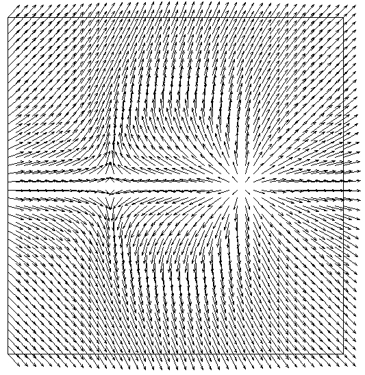
(a) $\|{\boldsymbol{d}}\|_{\infty}=0.9970543.$

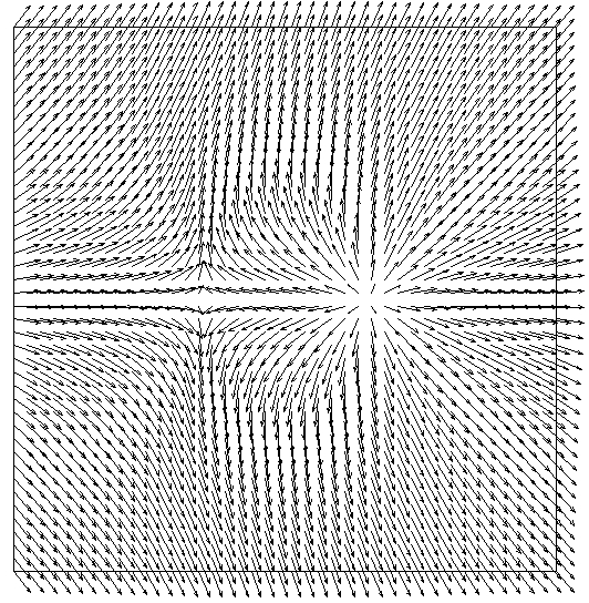
(b) $\|{\boldsymbol{d}}\|_{\infty}=0.9976057.$

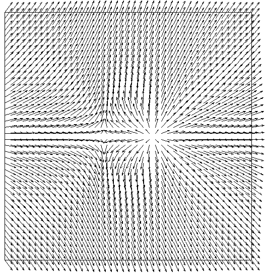
(c) $\|{\boldsymbol{d}}\|_{\infty}=0.9961038.$

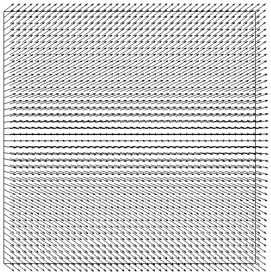
(d) $\|{\boldsymbol{d}}\|_{\infty}=0.9988512.$

Figure 1: Evolution of the director field at times $t=0.1,0.2,0,3$ and $0.6$.

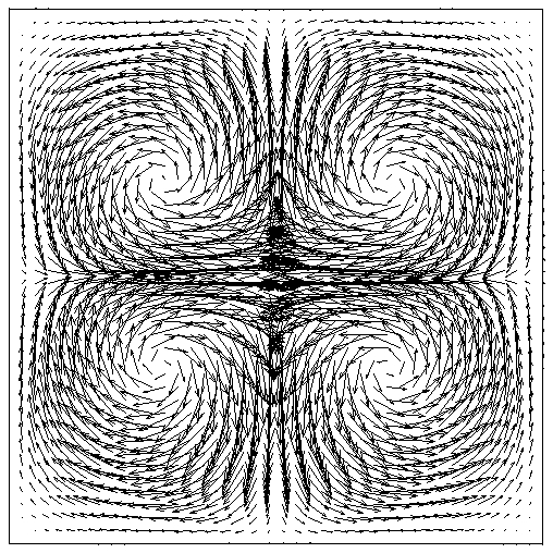
(a) $\|{\boldsymbol{v}}\|_{\infty}=0.2069006.$

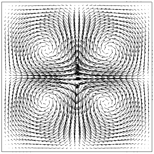
(b) $\|{\boldsymbol{v}}\|_{\infty}=0.1634978.$

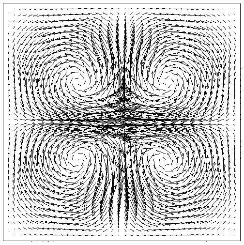
(c) $\|{\boldsymbol{v}}\|_{\infty}=0.2160761.$

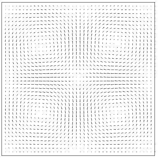
(d) $\|{\boldsymbol{v}}\|_{\infty}=0.001592144.$

Figure 2: Evolution of the velocity field at times $t=0.1,0.2,0,3$ and $0.6$. The relative size of the vectors were modified for better visualization.

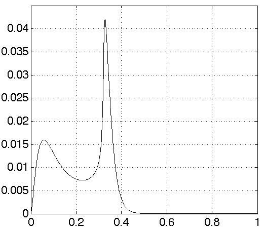
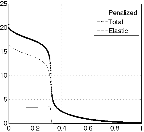
Figure 3: Energies for the experiment of singularities. Kinetic energy (left) and total, elastic and penalization energy (right)

6.2 Convergence rate

We are now interested in the accuracy with respect to time. In doing so, we consider $\Omega=(0,1)\times(-\frac{1}{2},\frac{1}{2})$ and $\lambda=\gamma=\nu=1$. The initial data are taken as

$${\boldsymbol{u}}_{0}=\boldsymbol{0},\mbox{ and }{\boldsymbol{d}}_{0}=(\sin(a),\cos(a)),\quad\mbox{ where }a=\pi(\cos(\pi x)+\sin(\pi y)).$$

which satisfies homogeneous Dirichlet conditions for the velocity field and homogeneous Neumann boundary conditions for the director field. The reference solution is taken as the numerical approximation computed with the parameters $(k,h,\varepsilon)=(1.5625\cdot 10^{-6},0.068986,0.05)$.

In Figure 4 and Table 1, we illustrate the error bevahiour and the convergence rate on the director, velocity and pressure fields measured in the $L^{2}(\Omega)$- and $H^{1}(\Omega)$-norm versus the time step. The tests have been performed by comparing our reference solution with the numerical approximation computed on five time-steps $k_{i+1}=0.5k_{i}$ for $i=1,2,3,4$ with $k_{1}=10^{-3}$.

The error on the velocity and director vector is of ${\mathcal{O}}(k)$ in the ${\boldsymbol{L}}^{2}(\Omega)$-norm, respectively, which is consistent with the results for the velocity in the context of the non-incremental projection method for the Navier-Stokes equations. The error on the director field in the ${\boldsymbol{H}}^{1}(\Omega)$-norm are of ${\mathcal{O}}(k)$, which means the splitting error associated to the segregation of the director field is the best that can be expected. Instead, the error on the velocity field in the ${\boldsymbol{H}}^{1}(\Omega)$-norm does not maintain the first-order accuracy from the beginning, which could mean that the theoretical order of approximation will be less than first-order. Furthermore, the error on the pressure in the $L^{2}(\Omega)$- and $H^{1}(\Omega)$-norm behaves as that on the velocity for the $H^{1}(\Omega)$-norm.

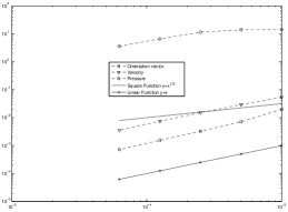
Figure 4: Evolution in time of the error in the $L^{2}(\Omega)$-norm (left) and the $H^{1}(\Omega)$-norm (right) for the director, velocity and pressure.

$k$	$L^{2}$-rate-$p$	${\boldsymbol{L}}^{2}$-rate-${\boldsymbol{v}}$	${\boldsymbol{L}}^{2}$-rate-${\boldsymbol{d}}$	$H^{1}$-rate-$p$	${\boldsymbol{H}}^{1}$-rate-${\boldsymbol{v}}$	${\boldsymbol{H}}^{1}$-rate-${\boldsymbol{d}}$
$10^{-3}$	–	–	–	–	–	–
$5\cdot 10^{-4}$	0.0295	0.8801	1.4751	0.0224	0.6581	1.5035
$2.5\cdot 10^{-4}$	0.2778	0.9517	1.1205	0.2601	0.8292	1.2142
$1.25\cdot 10^{-4}$	0.8017	1.0084	1.0698	0.7832	0.9261	1.1338
$6.25\cdot 10^{-5}$	0.8723	1.0783	1.1116	0.8742	1.0234	1.1396

Table 1: The convergence rates for the velocity, pressure and director

6.2.1 Dependence on parameters

As it is well-known for time-splitting schemes, conditions as those given in (H4) deteriorate the benefits of Scheme 5 because the number of linear systems to be solved increases when $(h,\varepsilon)$ are small. Thus one could think that these conditions reduce the efficiency of Scheme 5. However, as far as we are concerned, linear [20] and nonlinear [6] Euler time-stepping algorithms require such conditions. The former in order for numerical approximations to have a priori energy estimates, while the latter in order for the associated iterative process (e.g. Newton’s method) to be convergent. Therefore, we somehow have to impose conditions for $(k,h,\varepsilon)$, and hence that Scheme 5 is a good alternative for saving a lot of computational work in approximating (5).

To demonstrate the dependence of the numerical approximations on the discretization and penalization parameters according to the conditions given in $\rm(H4)$, we will test the sensitivity of Scheme 5 when varying the parameters $(k,h,\varepsilon)$. In doing so, we will consider the phenomenon of annihilation of singularities described above. In particular, we will focus on condition (11). Thus, define $\alpha=\frac{k}{h^{3/2}\varepsilon}$ and select $\varepsilon=5\times 10^{-2}$. We want to compute our numerical approximation for $(k,h)$ where $h=0.0912396,0.068986,0.0463677,0.0233754$ and $k=10^{-s}$ with $s=1,2,3,4$. The annihilation times $T_{A}$ reported in Table 2 are taken as those times where the value of the kinetic energy is maximum. In particular, we have observe that the total energy does not remain bounded as the parameter $\alpha$ becomes sufficiently large. That is, we find that our numerical approximations have no energy bounds. Therefore, Scheme 5 requires that the conditions given in $\rm(H4)$ holds in order to have a priori energy estimates in the presence of singularities.

$k\backslash h$	$0.0912396$	$0.068986$	$0.0463677$	$0.0233754$
	72.5697	110.379	200.312	559.617	$\alpha$
$10^{-1}$	✗	✗	✗	✗	Stab.
	$--$	$--$	$--$	$--$	$T_{A}$
	$--$	$--$	$--$	$--$	$E_{kin}$
	7.25697	11.0379	20.0312	55.9617	$\alpha$
$10^{-2}$	✗	✗	✗	✗	Stab.
	$--$	$--$	$--$	$--$	$T_{A}$
	$--$	$--$	$--$	$--$	$E_{kin}$
	0.725697	1.10379	2.00312	5.59617	$\alpha$
$10^{-3}$	✓	✓	✓	✓	Stab.
	0.322	0.328	0.334	0.338	$T_{A}$
	0.0422756	0.0420097	0.0418536	0.041728	$E_{kin}$
	0.0725697	0.110379	0.200312	0.559617	$\alpha$
$10^{-4}$	✓	✓	✓	✓	Stab.
	0.3046	0.3105	0.3154	0.3188	$T_{A}$
	0.0490944	0.0487923	0.0485807	0.0484494	$E_{kin}$

Table 2: Dependence of Scheme 5 on the parameters for the annihilation phenomenon with $\varepsilon=5\times 10^{-2}$ measured by the value of $\alpha=k/(h^{3/2}\varepsilon)$ with $h=0.0912396,0.068986,0.0463677,0.0233754$ and $k=10^{-s}$ with $s=1,2,3,4$. $T_{A}$ is the aniquilation time

References

- [1] F. Armero, J.C Simo. Formulation of a new class of fractional-step methods for the incompressible MHD equations that retains the long-term dissipativity of the continuum dynamical system. Fields Inst. Commun., 10 (1996).
- [2] S. Badia. On stabilized finite element methods based on the Scott-Zhang projector. Circumventing the inf-sup condition for the Stokes problem. Comput. Methods Appl. Mech. Engrg. 247/248 (2012), 65-72.
- [3] S. Badia, R. Planas, J. V. Gutiérrez-Santacreu. Unconditionally stable operator splitting algorithms for the incompressible magnetohydrodynamics system discretized by a stabilized finite element formulation based on projections. Internat. J. Numer. Methods Engrg. 93 (2013), no. 3, 302-328.
- [4] S. Badia, F. Guillén-Gonzalez, J. V. Gutiérrez-Santacreu. Finite element approximation of nematic liquid crystal flows using a saddle-point structure. J. Comput. Phys. 230 (2011), no. 4, 1686-1706.
- [5] S. Badia, F. Guillén-Gonzalez, J. V. Gutiérrez-Santacreu. An overview on numerical analyses of nematic liquid crystal flows. Arch. Comput. Methods Eng. 18 (2011), no. 3, 285-313.
- [6] R. Becker, X. Feng, A. Prohl. Finite element approximations of the Ericksen-Leslie model for nematic liquid crystal flow. SIAM J. Numer. Anal. 46 (2008), no. 4, 1704-1731.
- [7] S. Brenner, L. R. Scott. The Mathematical Theory of Finite Element Methods, TAM 15, Springer-Verlag, Berlin, 1994.
- [8] E. Burman, M.A. Fernández. Galerkin finite element methods with symmetric pressure stabilization for the transient Stokes equations: stability and convergence analysis, SIAM J. Numer. Anal. 47 (2008), no. 1, 409-439.
- [9] A. J. Chorin. Numerical solution of the Navier-Stokes equations. Math. Comp., 22 (1968) 745-762.
- [10] R. Codina, J. Blasco. A finite element formulation for the Stokes problem allowing equal velocity-pressure interpolation. Comput. Methods Appl. Mech. Engrg. 143 (1997), no. 3-4, 373-391.
- [11] R. Codina. Pressure stability in fractional step finite element methods for incompressible flows. J. Comput. Phys. 170 (2001), no. 1, 112-140.
- [12] C.L. Dohrmann, P.B. Bochev. A stabilized finite element method for the Stokes problem based on polynomial pressure projections. Int. J. Numer. Meth. Fluids. 46 (2004) 183-201.
- [13] J. Ericksen. Conservation laws for liquid crystals. Trans. Soc. Rheol., 5 (1961), 22-34.
- [14] J. Ericksen. Continuum theory of nematic liquid crystals. Res. Mechanica, 21 (1987), 381-392.
- [15] J. L. Ericksen. Liquid crystals with variable degree of orientation. Arch. Rational Mech. Anal. 113 (1990), no. 2, 97-120.
- [16] F. C. Frank. On the theory of liquid crystals. Discuss. Faraday Soc. 25, 19-28, 1958.
- [17] V. Girault, F. Guillén-González. Mixed formulation, approximation and decoupling algorithm for a nematic liquid crystals model. Math. Comput. 80 (2011), no. 274, 781-819.
- [18] J.-L. Guermond. Some practical implementations of projection methods for Navier-Stokes equations. Modél. Math. Anal. Num. 30 (1996), 637-667.
- [19] J.-L. Guermond, P. Minev, J. Shen. An overview of projection methods for incompressible flows. Comput. Methods Appl. Mech. Engrg. 195 (2006), 6011-6045
- [20] F. Guillén-Gonzalez, J. V. Gutiérrez-Santacreu. A linear mixed finite element scheme for a nematic Ericksen-Leslie liquid crystal model. ESAIM: M2AN. 47 (2013), no. 5, 1433-1464.
- [21] F. Hecht. New development in freefem++. J. Numer. Math. 20 (2012), no. 3-4, 251-265.
- [22] Q. Hu, X-C. Tai, R. Winther. A saddle-point approach to the computation of harmonic maps. SIAM J Numer Anal 47 (2009), no. 2, 1500-1523.
- [23] F. Leslie. Theory of flow phenomena in liquid crystals. The Theory of Liquid Crystals. W. Brown, ed. Academic Press, New York, 4 (1979), 1-81.
- [24] F. Leslie. Some constitutive equations for liquid crystals. Arch. Ration. Mech. Anal., 28 (1968), 265-283.
- [25] F.H. Lin. Nonlinear theory of defects in nematic liquid crystals: phase transition and flow phenomena. Comm. Pure Appl. Math., 42 (1989), 789-814.
- [26] F.H. Lin, C. Liu. Non-parabolic dissipative systems modelling the flow of liquid crystals. Comm. Pure Appl. Math. 48 (1995), 501-537.
- [27] F. H. Lin and C. Liu, Static and Dynamic Theories of Liquid Crystals. Journal of Partial Differential Equations, 14 (2001), no. 4, 289-330.
- [28] P. Lin, C. Liu. Simulations of singularity dynamics in liquid crystal flows: A finite element approach. Journal of Computational Physics 215 (2006) no. 2, 1411-1427.
- [29] P. Lin, C. Liu, H. Zhang. An energy law preserving finite element scheme for simulating the kinematic effects in liquid crystal flow dynamics. Journal of Computational Physics 227 (2007), 348-362.
- [30] C. Liu, N.J. Walkington. Mixed methods for the approximation of liquid crystal flows. M2AN Math. Model. Numer. Anal. 36 (2002), no. 2, 205-222.
- [31] C. Liu, N.J. Walkington. Approximation of liquid crystal flows. SIAM J. Numer. Anal. 37 (2000), no. 3, 725-741.
- [32] S. Minjeaud. An unconditionally stable uncoupled scheme for a triphasic Cahn- Hilliard/Navier-Stokes model. Num. Methods for PDE, 29 (2013), no. 2, 584-618.
- [33] C. Oseen. Theory of liquid crystals. Trans. Faraday Soc. 29, 883-899, 1933.
- [34] R. Rannacher. On Chorin’s projection method for incompressible Navier-Stokes equations. Lecture notes in mathematics, 1530 (1991), 167-183.
- [35] L. R. Scott, S. Zhang. Finite element interpolation of non-smooth functions satisfying boundary conditions. Math. Comp., 54, (1990), 483–493.
- [36] J. Shen. On error estimates of the projection methods for the Navier?Stokes equations: first-order schemes. SIAM J. Numer. Anal. 29 (1992) 57-77.
- [37] R. Temam. Sur l’approximation de la solution des équations de Navier-Stokes par la méthode des pas fractionnaires. Arch. Rational Mech. Anal., 33 (1969), 377-385.
- [38] R. Temam. Navier-Stokes equations, theory and numerical analysis. North-Holland, Amsterdam, 1979.