Nonequilibrium transport in a quantum dot attached to a Majorana bound state

Abstract

We investigate theoretically nonequilibrium quantum transport in a quantum dot attached to a Majorana bound state. Our approach is based on the Keldysh Green’s function formalism, which allows us to investigate the electric current continuously from the zero-bias limit up to the large bias regime. In particular, our findings fully agree with previous results in the literature that calculate transport using linear response theory (zero-bias) or the master equation (high bias). Our $I-V$ curves reveal a characteristic slope given by $I=(G_{0}/2)V$ in linear response regime, where $G_{0}$ is the ballistic conductance $e^{2}/h$ as predicted in Phys. Rev. B 84, 201308(R) (2011). Deviations from this behavior is also discussed when the dot couples asymmetrically to both left and right leads. The differential conductance obtained from the left or the right currents can be larger or smaller than $G_{0}/2$ depending on the strength of the coupling asymmetry. In particular, the standard conductance derived from the Landauer-Büttiker equation in linear response regime does not agree with the full nonequilibrium calculation, when the two leads couple asymmetrically to the quantum dot. We also compare the current through the quantum dot coupled to a regular fermionic (RF) zero-mode or to a Majorana bound state (MBS). The results differ considerably for the entire bias voltage range analyzed. Additionally, we observe the formation of a plateau in the characteristic $I-V$ curve for intermediate bias voltages when the dot is coupled to a MBS. Thermal effects are also considered. We note that when the temperature of the reservoirs is large enough both RF and MBS cases coincide for all bias voltages.

I Introduction

In 1937 Ettore Majorana realized that the Dirac equation could be modified to support a new class of particles called Majorana fermions (MFs), with the intriguing property that these particles are their own anti-particles.em37 ; JA12 Mathematically, if $\eta$ is the annihilation operator for a Majorana particle then $\eta=\eta^{\dagger}$. These exotic particles are non-abelian anyons, which means that particle exchanges are not merely accompanied by a $+1$ for bosons or a $-1$ for fermions that multiplies the wave function. Additionally, the exchange statistics of MFs does not follow the regular anyons observed as quasiparticles in 2D systems, where the exchange operation yields a Berry phase $e^{i\phi}$ multiplying the wave function.ml12 Thus we end up for MFs with an exotic non-Abelian exchange statistics. Until now no elementary particle on nature was found as a MF. There is one possibility that neutrinos might be MFs. On going experiments are attempting to verify this hypothesis.fw09 Despite its origin in high energy physics, MFs came recently in the news as a quasi-particle excitation in the low-energy field of solid state physics.ja13

Thus in the last few years the pursuit for devices hosting MFs has received much attention from the scientific community, in particular working with quantum computing. Such a quest is due to the possibility of bounding two far apart MFs in order to define a nonlocal qubit completely immune to the decoherence effect, which is crucial for the accomplishment of a robust topological quantum computer.ML11 ; Lu12 ; MLKF12 ; KF12 ; MLKF2012 To this end, experimental realizations should reveal first signatures of MFs that ensure the existence of them and hence, their application as essential blocks for quantum computing. Nowadays, the most promising setups for this goal lies on the superconductor based systems.AYK01 ; MG12 ; Lang12 ; Lin12 ; Liu13 ; DS13 ; JLiu12 ; SN13 ; DR12

For instance, it was recently measured as a MF signature a zero-bias peak in the conductance between a normal metal and the end of a semiconductor nanowire (InSb) that is attached to a s-wave superconductor.vm12 ; mtd12 This superconductor induces superconductivity in the InSb nanowire via the proximity effect. In the presence of a magnetic field parallel to the wire it was found a peak sticked at the midgap of the nontrivial topological superconductor. This peak is washed out for zero magnetic fields or when the magnetic field is parallel to the spin-orbit field of the wire. Additionally, this peak tends to disappear when temperature increases. All these features are in agreement with theoretical works that settle the ingredients necessary to have a Majorana bound state (MBS) in a hybrid nanowire-superconductor device.DLoss ; rml10 ; yo10 ; ktl09 ; jds10 However, an alternative explanations for these measurements were later proposed.tds12 Additionally, MF are expected to appear in a variety of solid state systems, namely, topological superconductorsJA12 and fractional quantum Hall systemsnr00 . Moreover, MFs are theoretically predicted to appear in a half-quantum vortex of a p-wave superconductorsDA01 or at the ends of supercondutor vortices in doped topological insulators.PPRA11

In solid state physics the main way to probe MBSs is via conductance. A few experiments use tunneling spectroscopy to probe MFs as a zero-bias anomaly. There are some theoretical proposals that deal with transport through a single level quantum dot attached to a left and to a right lead and to a MBS in the end of a quantum wire.del11 ; EV13 The main transport feature found for this system is a conductance peak pinned at zero-bias with an amplitude of one-half the ballistic conductance $G_{0}=e^{2}/h$,del11 valid when the left and right leads couple symmetrically to the dot. We point out that in Ref. [EV13, ], E. Vernek et al. have found that such a value arises from the leaking of the MBS into the quantum dot. Additionally, the transport in this system was investigated in the large bias regime, revealing a non-conserving current between left and right leads.yc12

In the present paper we apply the Keldysh nonequilibrium Green’s function techniquehh08 to extend these previous works to the whole bias voltage window, ranging from the zero-bias limit up to the large bias regime. So, instead of focusing only on the zero-bias anomaly, we explore the whole $I-V$ curve in the presence of a single MBS. For comparison we also show the results to the case of a regular fermionic (RF) zero-mode coupled to the dot. Both cases (MBS and RF) differ appreciably along the bias voltage window, not only in the zero-bias regime. We observe, for instance, the formation of an additional plateau in the I-V curve when the dot is coupled to a MBS. Additionally, it is found a slope at the characteristic $I-V$ curve equal to one-half the quantum of conductance $G_{0}$ when the bias voltage tends to zero, in accordance to Ref. [del11, ].

We pay particular attention to the coupling asymmetry between left lead-quantum dot and right lead-quantum dot. These couplings are characterized by the tunneling rates $\Gamma^{L}$ and $\Gamma^{R}$, respectively. We investigate the cases $\Gamma^{L}>\Gamma^{R}$ and $\Gamma^{L}<\Gamma^{R}$. Cao et al.yc12 found that in the large bias regime the current is not conserved with $I_{L}>I_{R}$ or $I_{L}<I_{R}$ depending on the asymmetry factor $y=\Gamma^{R}/\Gamma^{L}$. Interestingly, the nonconserving feature also affects the zero-bias conductance. The zero-bias limit departs from $G_{0}/2$ when the leads couple asymmetrically ($y\neq 1$) to the dot. We have found in the zero-bias limit $dI_{L}/dV>G_{0}/2$ and $dI_{R}/dV<G_{0}/2$ or the opposite, depending on the degree of asymmetry $y$. Neither $dI_{L}/dV$ nor $dI_{R}/dV$ coincide with the conductance obtained via the Landauer-Büttiker equation in linear response regime, except for symmetric couplings ($y=1$). This indicates that a full nonequilibrium quantum transport formulation is more suitable to describe the system with Majorana bound state. Thermal effects are also investigated. We observe that when the temperature is large enough both MBS and RF cases become indistinguishable for any bias voltage.

The paper is organized as follows. In Sec. II we present a detailed derivation of the nonlinear transport equations obtained via Keldysh technique. In Sec. III we show the main results found and in Sec. IV we conclude.

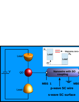
Figure 1: (Color online) Sketch of the system studied. A single level quantum dot is coupled to both left and right leads. In the presence of a bias voltage the system is driven away the equilibrium and a tunnel current passes through the dot. A semiconductor quantum wire (e.g. InSb) with strong spin orbit interaction lies on an s-wave superconductor that induces a topological phase in the wire, resulting in localized Majorana states at the ends of this wire, which is crossed by an applied magnetic field parallel to it and perpendicular to its spin-orbit field. The Majorana bound state closer to the dot couples to it, which can affect the characteristic $I-V$ profile.

II Model and Formulation

To describe the system presented in Fig. (1) we use the Hamiltonian originally proposed by Liu and Baranger,del11

$$H = H_{\text{leads}}+H_{\text{dot}}+H_{\text{T}}+\epsilon_{M}(f^{\dagger}f-\frac{1}{2})+$$ (1)

$$\frac{\lambda_{A}}{\sqrt{2}}(df^{\dagger}+fd^{\dagger})+\frac{\lambda_{B}}{\sqrt{2}}(df+f^{\dagger}d^{\dagger}),$$

where the first term gives the free-electron energy of the reservoirs, $H_{\text{leads}}=\sum_{k,\alpha}\varepsilon_{k}c_{k,\alpha}^{{\dagger}}c_{k,\alpha}$, the second term is the single level quantum dot Hamiltonian, $H_{dot}=\varepsilon_{d}d^{{\dagger}}d$ and the third term gives the tunnel coupling between the quantum dot and the leads, $H_{\text{T}}=\sum_{k,\alpha}[V_{\alpha}c_{k,\alpha}^{{\dagger}}d+V_{\alpha}^{*}d^{{\dagger}}c_{k,\alpha}]$, with $\alpha=L$ (left lead) or $\alpha=R$ (right lead). The fourth term accounts for the Majorana modes, and the last two terms can be understood as follows: (i) $\lambda_{A}=\lambda\neq 0$, $\lambda_{B}=0$ and $\epsilon_{M}=0$ we have a regular fermionic (RF) zero-mode attached to the quantum dot and (ii) for $\lambda_{A}=\lambda_{B}=\lambda$ we obtain a MBS coupled to the quantum dot. In case (i) the Hamiltonian becomes

$$H=H_{\text{leads}}+H_{\text{dot}}+H_{\text{T}}+\frac{\lambda}{\sqrt{2}}(df^{\dagger}+fd^{\dagger}),$$ (2)

while for (ii) we have

$$H=H_{\text{leads}}+H_{\text{dot}}+H_{\text{T}}+i\epsilon_{M}\eta_{1}\eta_{2}+\lambda(d-d^{\dagger})\eta_{1},$$ (3)

where $\eta_{1}=\frac{f^{\dagger}+f}{\sqrt{2}}$ and $\eta_{2}=i\frac{f^{\dagger}-f}{\sqrt{2}}$. In the following nonequilibrium calculation we consider this last Hamiltonian. In order to compare our findings with the ones obtained previously for the large bias limit, we adopt $\lambda=\sqrt{2}\lambda^{\prime}$, where $\lambda^{\prime}$ gives the tunnel coupling between the dot and the nearby MBS in Ref. [yc12, ]. We highlight that the present spinless Hamiltonian for MFs assumes a strong magnetic field applied on the whole setup of Fig. (1), thus resulting a large Zeeman splitting where the higher levels are not energetic favorable within the operational temperatures of the system. In this case, one spin component becomes completely inert and the spin degrees of freedom can be safely ignored. As a result, the Coulomb interaction between opposite spins in the quantum dot is avoided and the model becomes exactly solvable. To our best knowledge, this work is the first to obtain such a solution by using Green’s functions in the Keldysh framework.

The current in the lead $\alpha$ can be calculated from the definition $I_{\alpha}=-e\langle\dot{N}_{\alpha}\rangle$, where $e>0$ is the modulus of the electron charge. $N_{\alpha}=\sum_{k}c_{k\alpha}^{\dagger}c_{k\alpha}$ is the total number operator for lead $\alpha$ and $\langle...\rangle$ is a thermodynamics average. The time derivative of $N_{\alpha}$ is calculated via Heisenberg equation, $\dot{N}_{\alpha}=i[H,N_{\alpha}]$ (we adopt $\hbar=1$), which results inhh08

$$I_{\alpha}=2e\mathrm{Re}[\sum_{k_{a}}V_{\alpha}G_{d,k_{\alpha}}^{<}(t,t)],$$ (4)

where $G_{d,k_{\alpha}}^{<}(t,t)=i\langle c_{k_{\alpha}}^{\dagger}(t)d(t)\rangle$. After a straightforward calculation the current expression can be cast into the following form

$$I_{\alpha}=ie\int\frac{d\omega}{2\pi}\Gamma_{\alpha}\{[G_{d}^{r}(\omega)-G_{d}^{a}(\omega)]f_{\alpha}+G_{d}^{<}(\omega)\}.$$ (5)

Here $\Gamma_{\alpha}=2\pi V_{\alpha}^{2}\rho_{\alpha}$, with $\rho_{\alpha}$ being the density of states of the reservoir $\alpha$, and the Green’s functions $G_{d}^{r}(\omega)$, $G_{d}^{a}(\omega)$ and $G_{d}^{<}(\omega)$ are the retarded, advanced and lesser Green’s functions of the quantum dot. These Green’s functions can be obtained via analytic continuation of the contour-ordered Green’s functions $G_{d}(\tau,\tau^{\prime})=-i\langle T_{c}d(\tau)d^{\dagger}(\tau^{\prime})\rangle$, where $T_{c}$ orders the operators along the Keldysh contour. Since the equation of motion for $G_{d}(\tau,\tau^{\prime})$ is structurally equivalent to the chronological time-ordered Green’s function $G_{d}(t,t^{\prime})=-i\langle Td(t)d^{\dagger}(t^{\prime})\rangle$,hh08 in what follows we calculate $G_{d}(t,t^{\prime})$ via equation of motion technique. Taking the time derivative with respect to $t$ we obtain

$$[i\frac{\partial}{\partial t}-\varepsilon_{d}]G_{d}(t,t^{\prime}) = \delta(t-t^{\prime})+\sum_{k,\alpha}V_{\alpha}^{*}G_{c_{k\alpha}}(t,t^{\prime})$$ (6)

$$\phantom{xxxxxx}-\lambda G_{\eta_{1}}(t,t^{\prime}),$$

where the additional Green’s functions were defined as $G_{c_{k\alpha}}(t,t^{\prime})=-i\langle Tc_{k\alpha}(t)d^{\dagger}(t^{\prime})\rangle$ and $G_{\eta_{1}}(t,t^{\prime})=-i\langle T\eta_{1}(t)d^{\dagger}(t^{\prime})\rangle$. Calculating the time-derivative of these new Green’s function with respect to $t$ we find

$$[i\frac{\partial}{\partial t}-\varepsilon_{k,\alpha}]G_{c_{k\alpha}}(t,t^{\prime})=V_{\alpha}G_{d}(t,t^{\prime}),$$ (7)

and

$$i\frac{\partial}{\partial t}G_{\eta_{1}}(t,t^{\prime})=i\varepsilon_{M}G_{\eta_{2}}(t,t^{\prime})-\lambda G_{d}(t,t^{\prime})+\lambda G_{d^{\dagger}}(t,t^{\prime}).$$

(8)

Observe that two new Green’s functions arise at this last equation, namely, $G_{\eta_{2}}(t,t^{\prime})=-i\langle T\eta_{2}(t)d^{\dagger}(t^{\prime})\rangle$ and $G_{d^{\dagger}}(t,t^{\prime})=-i\langle Td^{\dagger}(t)d^{\dagger}(t^{\prime})\rangle$. Performing once again the time-derivative with respect to $t$ of these two Green’s functions we arrive at

$$i\frac{\partial}{\partial t}G_{\eta_{2}}(t,t^{\prime})=-i\varepsilon_{M}G_{\eta_{1}}(t,t^{\prime}),$$ (9)

and

$$[i\frac{\partial}{\partial t}+\varepsilon_{d}]G_{d^{{\dagger}}}(t,t^{\prime})=-\sum_{k,\alpha}V_{\alpha}G_{c_{k\alpha}^{\dagger}}(t,t^{\prime})+\lambda G_{\eta_{1}}(t,t^{\prime}).$$

(10)

One more Green’s function appears at this last results, $G_{c_{k\alpha}^{\dagger}}(t,t^{\prime})=-i\langle Tc_{k\alpha}^{\dagger}(t)d^{\dagger}(t^{\prime})\rangle$, whose equation of motion can be easily calculated,

$$[i\frac{\partial}{\partial t}+\varepsilon_{k\alpha}]G_{c_{k\alpha}^{\dagger}}(t,t^{\prime})=-V_{\alpha}^{*}G_{d^{{\dagger}}}(t,t^{\prime}).$$ (11)

Equations (6), (7), (8), (9), (10) and (11) constitute a complete set of six differential equations. In order to reduce to only four equations we write Eqs. (7) and (11) in their integral formscomment1

$$G_{c_{k\alpha}}(t,t^{\prime}) = V_{\alpha}\int dt_{1}g_{k\alpha}(t,t_{1})G_{d}(t_{1},t^{\prime}),$$ (12)

$$G_{c_{k\alpha}^{\dagger}}(t,t^{\prime}) = -V_{\alpha}^{*}\int dt_{1}g^{\prime}_{k\alpha}(t,t_{1})G_{d^{{\dagger}}}(t,t^{\prime})$$ (13)

and use them into Eqs. (6) and (10). This gives us

$$[i\frac{\partial}{\partial t}-\varepsilon_{d}]G_{d}(t,t^{\prime}) = \delta(t-t^{\prime})+\int dt_{1}\Sigma(t,t_{1})G_{d}(t_{1},t^{\prime})$$ (14)

$$\phantom{xxxxxx}-\lambda G_{\eta_{1}}(t,t^{\prime}),$$

and

$$[i\frac{\partial}{\partial t}+\varepsilon_{d}]G_{d^{{\dagger}}}(t,t^{\prime}) = \int dt_{1}\Sigma^{\prime}(t,t_{1})G_{d^{{\dagger}}}(t_{1},t^{\prime})$$

$$\phantom{xxxxxx}+\lambda G_{\eta_{1}}(t,t^{\prime}),$$

where $\Sigma(t,t_{1})=\sum_{k\alpha}|V_{\alpha}|^{2}g_{k\alpha}(t,t_{1})$ and $\Sigma^{\prime}(t,t_{1})=\sum_{k\alpha}|V_{\alpha}|^{2}g^{\prime}_{k\alpha}(t,t_{1})$. Equations (8), (9), (14) and (LABEL:Gddaggerint) constitute our new set of four-integrodifferential equations, which can be written in a matrix form as

$$\left[\begin{array}[]{cccc}i\frac{\partial}{\partial t}-\varepsilon_{d}&0&0&0\\ 0&i\frac{\partial}{\partial t}&0&0\\ 0&0&i\frac{\partial}{\partial t}&0\\ 0&0&o&i\frac{\partial}{\partial t}+\varepsilon_{d}\\ \end{array}\right]\left[\begin{array}[]{c}G_{d}(t,t^{\prime})\\ G_{\eta_{1}}(t,t^{\prime})\\ G_{\eta_{2}}(t,t^{\prime})\\ G_{d^{\dagger}}(t,t^{\prime})\\ \end{array}\right] = \delta(t-t^{\prime})\left[\begin{array}[]{c}1\\ 0\\ 0\\ 0\\ \end{array}\right]+\int dt_{1}\left[\begin{array}[]{cccc}\Sigma(t,t_{1})&0&0&0\\ 0&0&0&0\\ 0&0&0&0\\ 0&0&0&\Sigma^{\prime}(t,t_{1})\\ \end{array}\right]\left[\begin{array}[]{c}G_{d}(t_{1},t^{\prime})\\ G_{\eta_{1}}(t_{1},t^{\prime})\\ G_{\eta_{2}}(t_{1},t^{\prime})\\ G_{d^{\dagger}}(t_{1},t^{\prime})\\ \end{array}\right]+$$ (45)

$$\phantom{xxxxxxxxxxxx}\left[\begin{array}[]{cccc}0&-\lambda&0&0\\ -\lambda&0&i\varepsilon_{M}&\lambda\\ 0&-i\varepsilon_{M}&0&0\\ 0&\lambda&0&0\\ \end{array}\right]\left[\begin{array}[]{c}G_{d}(t,t^{\prime})\\ G_{\eta_{1}}(t,t^{\prime})\\ G_{\eta_{2}}(t,t^{\prime})\\ G_{d^{\dagger}}(t,t^{\prime})\\ \end{array}\right],$$

or in a more compact way as

$$\vec{G}(t,t^{\prime})=\mathbf{g}(t,t^{\prime})\vec{u}+\int\int dt_{1}dt_{2}\mathbf{g}(t,t_{1})\widetilde{\mathbf{\Sigma}}(t_{1},t_{2})\vec{G}(t_{2},t^{\prime}),$$

where the matrix $\mathbf{g}(t,t^{\prime})$ is defined according to

$$\left[\begin{array}[]{cccc}i\frac{\partial}{\partial t}-\varepsilon_{d}&0&0&0\\ 0&i\frac{\partial}{\partial t}&0&0\\ 0&0&i\frac{\partial}{\partial t}&0\\ 0&0&o&i\frac{\partial}{\partial t}+\varepsilon_{d}\\ \end{array}\right]\mathbf{g}(t,t^{\prime})=\delta(t-t^{\prime})\mathbf{I},$$ (51)

with $\mathbf{I}$ being the $4\times 4$ identity matrix, and

$$\widetilde{\mathbf{\Sigma}}(t,t^{\prime}) = \left[\begin{array}[]{cccc}\Sigma(t,t^{\prime})&0&0&0\\ 0&0&0&0\\ 0&0&0&0\\ 0&0&0&\Sigma^{\prime}(t,t^{\prime})\\ \end{array}\right]+$$ (62)

$$\delta(t-t^{\prime})\left[\begin{array}[]{cccc}0&-\lambda&0&0\\ -\lambda&0&i\varepsilon_{M}&\lambda\\ 0&-i\varepsilon_{M}&0&0\\ 0&\lambda&0&0\\ \end{array}\right].$$

The vectors $\vec{G}$ and $\vec{u}$ are defined as

$$\vec{G}(t,t^{\prime})=\left[\begin{array}[]{c}G_{d}(t,t^{\prime})\\ G_{\eta_{1}}(t,t^{\prime})\\ G_{\eta_{2}}(t,t^{\prime})\\ G_{d^{\dagger}}(t,t^{\prime})\\ \end{array}\right]\phantom{xxx}\mathrm{and}\phantom{xxx}\vec{u}=\left[\begin{array}[]{c}1\\ 0\\ 0\\ 0\\ \end{array}\right].$$ (63)

Iterating Eq. (II) we can show that

$$\vec{G}(t,t^{\prime})=\mathbf{G}(t,t^{\prime})\vec{u},$$ (64)

with the Dyson equation

$$\mathbf{G}(t,t^{\prime})=\mathbf{g}(t,t^{\prime})+\int\int dt_{1}dt_{2}\mathbf{g}(t,t_{1})\widetilde{\mathbf{\Sigma}}(t_{1},t_{2})\mathbf{G}(t_{2},t^{\prime}).$$

Writing a similar equation in the Keldysh contour,hh08

$$\mathbf{G}(\tau,\tau^{\prime})=\mathbf{g}(\tau,\tau^{\prime})+\int_{C}\int_{C}d\tau_{1}d\tau_{2}\mathbf{g}(\tau,\tau_{1})\widetilde{\mathbf{\Sigma}}(\tau_{1},\tau_{2})\mathbf{G}(\tau_{2},\tau^{\prime}),$$

and applying the Langreth’s analytical continuation rules,hh08 we obtain in the frequency domain

$$\mathbf{G}^{r}(\omega)=\mathbf{g}^{r}(\omega)+\mathbf{g}^{r}(\omega)\widetilde{\mathbf{\Sigma}}^{r}(\omega)\mathbf{G}^{r}(\omega),$$ (67)

to the retarded Green’s function and

$$\mathbf{G}^{<}(\omega)=\mathbf{G}^{r}(\omega){\mathbf{\Sigma}}^{<}(\omega)\mathbf{G}^{a}(\omega),$$ (68)

to the lesser Green’s function both already in the Fourier domain. The retarded and lesser components of the self-energy can be expressed as

$$\widetilde{\mathbf{\Sigma}}^{r}(\omega)=\left[\begin{array}[]{cccc}-\frac{i}{2}\Gamma(\omega)&-\lambda&0&0\\ -\lambda&0&i\varepsilon_{M}&\lambda\\ 0&-i\varepsilon_{M}&0&0\\ 0&\lambda&0&-\frac{i}{2}\Gamma(-\omega)\\ \end{array}\right],$$ (69)

and ${\mathbf{\Sigma}}^{<}(\omega)$ has only two nonzero elements,

$${{\Sigma}}^{<}_{11}(\omega) = i[\Gamma_{L}(\omega)f_{L}(\omega)+\Gamma_{R}(\omega)f_{R}(\omega)],$$ (70)

$${{\Sigma}}^{<}_{44}(\omega) = i[\Gamma_{L}(-\omega)f_{L}(-\omega)+\Gamma_{R}(-\omega)f_{R}(-\omega)],$$ (71)

With Eqs. (67) and (68) we can calculate the transport properties described below.

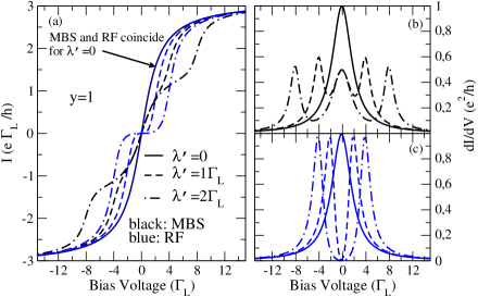
Figure 2: (Color online) (a) Current and differential conductance against the bias voltage in units of $\Gamma_{L}$ for differing $\lambda^{\prime}$ and symmetric case $y=1$. Both MBS and RF cases are shown, as black and blue lines, respectively. The $\lambda^{\prime}=0$ gives the same results for both cases, which corresponds to a transport through a single level quantum dot. For finite $\lambda^{\prime}$ the two cases present distinct $I-V$ profiles. The RF case shows a flat $I-V$ characteristics around zero bias and then it increases when the double-dot conduction channels cross the reservoir chemical potential. Contrasting, the MBS regime yields a typical slope around zero bias which turns into the $G_{0}/2$ as predicted in the literature. In panels (b)-(c) we show $dI/dV$ for both cases. While in the MBS the conductance is pinned at 0.5 $(\lambda^{\prime}\neq 0)$ it is zero in the RF regime. Parameters: $y=1$, $\Gamma_{R}=y\Gamma_{L}$, $k_{B}T=0.01\Gamma_{L}$, $\epsilon_{M}=0$, $\epsilon_{d}=0$, $\lambda^{\prime}=0$, $1\Gamma_{L}$ and $2\Gamma_{L}$, $\lambda=\sqrt{2}\lambda^{\prime}$.

III Results

In Fig. 2(a) we compare the characteristic $I-V$ curve in the cases of a MBS and a RF attached to the quantum dot. We adopt $\Gamma_{L}$ as our energy scale, so the bias voltage, the energy levels, and the coupling $\lambda^{\prime}$ will be expressed in units of $\Gamma_{L}$, while the currents in units of $e\Gamma_{L}/h$, with $h$ being the Planck’s constant. For $\lambda=0$ both results coincide and the system behaves as a single level quantum dot. For $\lambda\neq 0$ distinct features arise in each case. In particular, in the linear response regime, the current presents a finite slope as the bias increases for the MBS case while it is flat for the RF situation. As the bias voltage increases above the linear response regime, we observe the formation of a plateau in the current for the MBS case and then it increases further, saturating at large enough bias voltages. In contrast, for $\lambda_{B}=0$ (RF) we have a single step current profile, without the formation of an intermediate plateau. For larger biases the current coincides for both cases (RF and MBS).

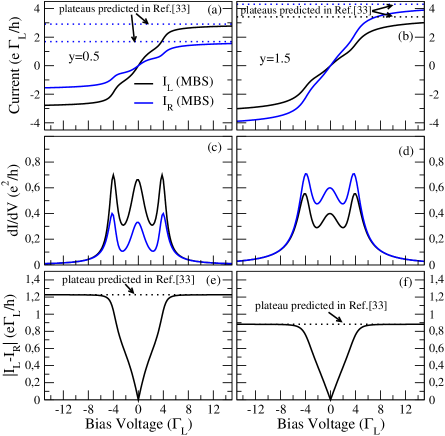
Figure 3: (Color online) (a)-(b) Left and right lead currents, (c)-(d) differential conductance $dI/dV$ and (e)-(f) current difference $|I_{L}-I_{R}|$ against the bias voltage in energy units of $\Gamma_{L}$. We consider $y=0.5$ (left panels) and $y=1.5$ (right panels). Both $I_{L}$ and $I_{R}$ present similar features against bias voltage but distinct values. In particular the slope around zero bias and the plateaus differ from each other. In order to confirm our nonequilibrium calculation we compare the high bias plateau with the ones predicted by Cao et al.yc12 via the master equation technique. The different $|I_{L}-I_{R}|$ increases with bias and then it saturates at the value predicted in the aforementioned reference. The zero bias value of the differential conductance $dI/dV$ contrasts to the one obtained for the symmetric case $y=1$. Here $dI_{L}/dV$ and $dI_{R}/dV$ are not at 0.5 and they differ from each other, with $dI_{L}/dV>dI_{R}/dV$ for $y<1$ and the opposite for $y>1$. Parameters: $\Gamma_{R}=y\Gamma_{L}$, $k_{B}T=0.01\Gamma_{L}$, $\epsilon_{M}=0$, $\epsilon_{d}=0$, $\lambda^{\prime}=1\Gamma_{L}$.

In Fig. 2(b) we show the differential conductance ($dI/dV$) for the currents presented in Fig. 2(a) in the presence of a MBS. For $\lambda=0$ the conductance $dI/dV$ is the standard Lorentzian with broadening given by $\Gamma=\Gamma_{L}+\Gamma_{R}$. In contrast, for $\lambda\neq 0$ the conductance reveals a three peaks structure, in which one of them has an amplitude of 0.5 pinned at zero-bias, in accordance to the work of Liu and Baranger.del11 For the RF, though, we find $dI/dV$ similar to the characteristic T-shaped quantum dot geometry,ACS09 where the conductance is zero for bias voltage close to zero.

It is valid to note that the currents presented in Fig. (2) for both MBS and RF cases can also be obtained from the standard Landauer-Büttiker expressioncomment2

$$I=\frac{e}{\hbar}\int\frac{d\omega}{2\pi}[f_{L}(\omega)-f_{R}(\omega)]T(\omega),$$ (72)

where $T(\omega)=[\Gamma_{L}\Gamma_{R}/(\Gamma_{L}+\Gamma_{R})](-2)\text{{Im}}[G_{dd}^{r}(\omega)]$, which gives the following conductance in the linear response limit

$$G=\frac{e^{2}}{h}\int d\omega\frac{\Gamma_{L}\Gamma_{R}}{\Gamma_{L}+\Gamma_{R}}(-2)\text{{Im}}[G_{dd}^{r}(\omega)][-\frac{\partial f}{\partial\omega}].$$ (73)

This symmetric expression is only true for charge conserving systems where $I_{L}=-I_{R}$. This is always the case when $\lambda_{B}=0$ (RF). However, for $\lambda_{B}=\lambda_{A}\neq 0$ (MBS) this is valid in the symmetric coupling regime ($y=1$) only. When $y\neq 1$ the left and right currents depart from each other, and consequently the result obtained from Eq. (72) differs from both $I_{L}$ and $I_{R}$ obtained via Eq. (5).

In order to explore the coupling asymmetries ($y\neq 1$) in the transport, we plot separately in Fig. (3) both $I_{L}$ and $I_{R}$ for $\lambda_{B}=\lambda_{A}=\lambda$ (MBS), and their corresponding $dI/dV$ profiles for two asymmetry factors $y=0.5$ (left panels) and $y=1.5$ (right panels). It is clear from the plot that the system does not conserve current ($I_{L}\neq I_{R}$). For larger enough bias voltages the currents $I_{L}$ and $I_{R}$ attain different plateaus, which are confirmed by the analytical results, recently derived by Cao et al. via Born-Markov master equation technique, namely,yc12

$$I_{L} = \frac{\Gamma_{L}\Gamma_{R}}{\Gamma}[1+\frac{4(1/y-1)\lambda^{\prime 2}}{\Gamma^{2}+4(\epsilon_{d}^{2}+\epsilon_{M}^{2}+2\lambda^{\prime 2})}],$$ (74)

$$I_{R} = \frac{\Gamma_{L}\Gamma_{R}}{\Gamma}[1+\frac{4(y-1)\lambda^{\prime 2}}{\Gamma^{2}+4(\epsilon_{d}^{2}+\epsilon_{M}^{2}+2\lambda^{\prime 2})}].$$ (75)

These large bias limiting values are plotted in Fig. (3) as dotted lines. Looking at the zero-bias limit, one may note that the slopes of $I_{L}$ and $I_{R}$ vs. $V$ deviate from each other with $|I_{L}|>|I_{R}|$ for $y=0.5$ and $|I_{L}|<|I_{R}|$ for $y=1.5$. The differential conductance $dI_{L}/dV$ and $dI_{R}/dV$ clearly show the difference of the slopes at zero bias, with $dI_{L}/dV\approx 0.7$ and $dI_{R}/dV\approx 0.3$ for $y=0.5$ and $dI_{L}/dV\approx 0.4$ and $dI_{R}/dV\approx 0.6$ for $y=1.5$. This contrasts with the symmetric case, where both conductances are at 0.5, as predicted by Liu and Baranger.del11

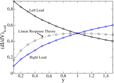
Figure 4: (Color online) (a) Differential conductances $dI_{L}/dV$ and $dI_{R}/dV$ at zero-bias against $y$ in the presence of a MBS. $dI_{L}/dV$ is larger than $dI_{R}/dV$ for small $y$, they attain the same value at $y=1$ and then $dI_{R}/dV$ turns greater than $dI_{L}/dV$ as $y$ becomes higher than one. For comparison we show $dI/dV$ obtained via linear response theory. Parameters: $\Gamma_{R}=y\Gamma_{L}$, $k_{B}T=0.01\Gamma_{L}$, $\epsilon_{M}=0$, $\epsilon_{d}=0$, $\lambda^{\prime}=1\Gamma_{L}$.

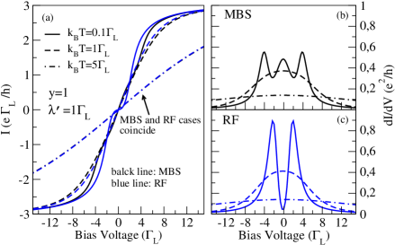
Figure 5: (Color online) (a) Current and (b)-(c) differential conductance against the bias voltage for three values of temperature: $k_{B}T=0.1\Gamma_{L}$, $1\Gamma_{L}$ and $5\Gamma_{L}$. Both MBS and RF cases are shown. For small temperatures both cases differ, however as $k_{B}T$ increases the two regimes tend to the same results. In particular, the characteristic signature $dI/dV=0.5G_{0}$ for a MBS is washed out as the temperature enhances. Parameters: $y=1$, $\Gamma_{R}=y\Gamma_{L}$, $\epsilon_{M}=0$, $\epsilon_{d}=0$, $\lambda^{\prime}=1\Gamma_{L}$.

In Fig. 3(e)-(f) we plot the difference $|I_{L}-I_{R}|$ against bias voltage. It is clear that in the nonequilibrium regime the current is not conserved with $I_{L}>I_{R}$ for $y<1$ and the opposite for $y>1$. As the bias voltage enlarges and all the conduction channels (three channels in the presence of a MBS) become inside the conduction window, the difference $|I_{L}-I_{R}|$ attains the plateau predicted by Eqs. (74)-(75).

In Fig. (4) we show how $dI/dV$ evolves with $y$ at the zero-bias limit. Both $dI_{L}/dV$ (black) and $dI_{R}/dV$ (blue) are shown. As a matter of comparison we also plot $dI/dV$ obtained via the standard linear response expression, Eq. (73). While all results coincide for the symmetric case ($y=1$), they all differ for $y\neq 1$.

Finally, Fig. (5) shows $I$ vs. $V$ curves and the corresponding differential conductance for different temperatures in the symmetric case ($y=1$). Both the MBS and RF cases are presented. As the temperature increases the curves for both regimes tend to become smoother, as expected due to the smearing out of the Fermi function around the chemical potential of the electronic reservoirs. In particular, opposite behavior between MBS and RF are seen at the slope of the $I-V$ curve around zero bias. While in the MBS the slope is suppressed for increasing $k_{B}T$, it is amplified in the RF case for $k_{B}T=1\Gamma_{L}$. This behavior can be clearly seen in the differential conductance $dI/dV$ at zero bias. Remarkably, both MBS and RF cases coincide for large enough temperature and the $I-V$ presents a linear profile.

IV Conclusion

We have studied nonequilibrium quantum transport in a quantum dot attached to two leads and to a localized Majorana bound state. Our approach, based on the Keldysh nonequilibrium Green’s function, allows us to study transport through the whole bias voltage range, starting at the zero-bias limit and moving up to the large bias regime. Previous works investigate separately only the zero-bias or the large bias limit. To the best of our knowledge this is the first work that covers the entire bias window. Our findings include the characteristic slope of $G_{0}/2$ in the $I-V$ profile at the zero-bias limit when the two leads couple symmetrically to the quantum dot, in accordance to the prediction of Ref. [del11, ]. However, in the asymmetric case ($y\neq 1$) we find a deviation from this slope, with $dI_{L}/dV>G_{0}/2$ and $dI_{R}/dV<G_{0}/2$ or the opposite, depending on the degree of asymmetry. We also compare both $dI_{L}/dV$ and $dI_{R}/dV$ with the conductance obtained via Eq. (73). They all agree only for symmetric coupling ($y=1$). This indicates that a full nonequilibrium quantum transport formulation is required to a better description of the system. Our results were also compared to those expected when a quantum dot is coupled to a RF zero-mode, instead of a MBS. The two cases (RF and MBS) differ appreciably in the entire bias-voltage range, not only at the zero bias regime. Additionally, we observe the formation of a plateau in the $I-V$ profile for intermediate bias voltages when the dot is coupled to a MBS. This plateau is not seen in the RF case. We also note that when the reservoirs temperature is large enough the two cases coincide, thus becoming indistinguishable via transport measurements if the dot is attached to a RF level or to a MBS.

References

- (1) E. Majorana, Nuovo Cimento 5, 171 (1937).
- (2) J. Alicea, Rep. Prog. Phys. 75, 076501 (2012).
- (3) M. Leijnse and K. Flensberg, Semicond. Sci. Technol. 27, 124003 (2012).
- (4) For a short review see F. Wilczek, Nature Phys. 5, 614 (2009).
- (5) J. Alicea, Nat. Nanotech. 8, 623 (2013).
- (6) M. Leijnse and K. Flensberg, Phys. Rev. B 84, 140501(R) (2011).
- (7) H.- F. Lu, H.- Z. Lu, and S.- Q. Shen, Phys. Rev. B 86, 075318 (2012).
- (8) M. Leijnse and K. Flensberg, Phys. Rev. B 86, 134528 (2012).
- (9) K. Flensberg, Phys. Rev. Lett. 106, 090503 (2011).
- (10) M. Leijnse and K. Flensberg, Phys. Rev. Lett. 107, 210502 (2011).
- (11) A. Y. Kitaev, Phys. Usp. 44, 131 (2001).
- (12) M. Gibertini, F. Taddei, M. Polini, and R. Fazio, Phys. Rev. B 85, 144525 (2012).
- (13) L.- J. Lang and S. Chen, Phys. Rev. B 86, 205135 (2012).
- (14) C.- H. Lin, J. D. Sau, and S. Das Sarma, Phys. Rev. B 86, 224511 (2012).
- (15) X.- J. Liu and A. M. Lobos, Phys. Rev. B 87, 060504(R) (2013).
- (16) D. Sticlet, C. Bena, and P. Simon, Phys. Rev. B 87, 104509 (2013).
- (17) J. Liu, A. C. Potter, K. T. Law, and P. A. Lee, Phys. Rev. Lett. 109, 267002 (2012).
- (18) S. Nakosai, J. C. Budich, Y. Tanaka, B. Trauzettel, and N. Nagaosa, Phys. Rev. Lett. 110, 117002 (2013).
- (19) D. Roy, C. J. Bolech, and N. Shah, Phys. Rev. B 86, 094503 (2012).
- (20) V. Mourik, K. Zuo, S. M. Frolov, S. R. Plissard, E. P. A. M. Bakkers, L. P. Kouwenhoven, Science 336, 1003 (2012).
- (21) M. T. Deng, C. L. Yu, G. Y. Huang, M. Larsson, P. Caroff, and H. Q. Xu, Nano Lett. 12, 6414 (2012).
- (22) A. A. Zyuzin, D. Rainis, J. Klinovaja, and D. Loss, Phys. Rev. Lett. 111, 056802 (2013).
- (23) R. M. Lutchyn, J. D. Sau, and S. Das Sarma, Phys. Rev. Lett. 105, 077001 (2010).
- (24) Y. Oreg, G. Refael, and F. von Oppen, Phys. Rev. Lett. 105, 177002 (2010).
- (25) K. T. Law, P. A. Lee, and T. K. Ng, Phys. Rev. Lett. 103, 237001 (2009).
- (26) J. D. Sau, S. Tewari, R. M. Lutchyn, T. D. Stanescu, and S. Das Sarma, Phys. Rev. B 82, 214509 (2010).
- (27) T. D. Stanescu, S. Tewari, J. D. Sau, and S. Das Sarma, Phys. Rev. Lett. 109, 266402 (2012).
- (28) N. Read and D. Green, Phys. Rev. B 61, 10267 (2000).
- (29) D. A. Ivanov, Phys. Rev.Lett. 86, 268 (2001).
- (30) P. Hosur, P. Ghaemi, R. S. K. Mong, and A. Vishwanath, Phys. Rev. Lett. 107, 097001 (2011).
- (31) D. E. Liu and H. U. Baranger, Phys. Rev. B 84, 201308(R) (2011).
- (32) E. Vernek, P. H. Penteado, A. C. Seridonio and J. C. Egues, arXiv: 1308.0092v2 [cond-mat.mes-hall] (2013).
- (33) Y. Cao, P. Wang, G. Xiong, M. Gong, and X.-Q. Li, Phys. Rev. B 86, 115311 (2012).
- (34) H. Haug and A. P. Jauho, Quantum Kinetics in Transport and Optics of Semiconductors, Springer Series in Solid-State Sciences 123, Second Edition, 2008.
-
(35)
In these equations we have used the definitions
and(76) (77) - (36) A. C. Seridonio, M. Yoshida, and L. N. Oliveira, Euro Phys. Lett. 86, 67006 (2009).
- (37) In the next two expressions we write explicitly or .