FACT – The G-APD revolution
in Cherenkov astronomy

Abstract

Since two years, the FACT telescope is operating on the Canary Island of La Palma. Apart from its purpose to serve as a monitoring facility for the brightest TeV blazars, it was built as a major step to establish solid state photon counters as detectors in Cherenkov astronomy. The camera of the First G-APD Cherenkov Telesope comprises 1440 Geiger-mode avalanche photo diodes (G-APD), equipped with solid light guides to increase the effective light collection area of each sensor. Since no sense-line is available, a special challenge is to keep the applied voltage stable although the current drawn by the G-APD depends on the flux of night-sky background photons significantly varying with ambient light conditions. Methods have been developed to keep the temperature and voltage dependent response of the G-APDs stable during operation. As a cross-check, dark count spectra with high statistics have been taken under different environmental conditions. In this presentation, the project, the developed methods and the experience from two years of operation of the first G-APD based camera in Cherenkov astronomy under changing environmental conditions will be presented.

I Introduction

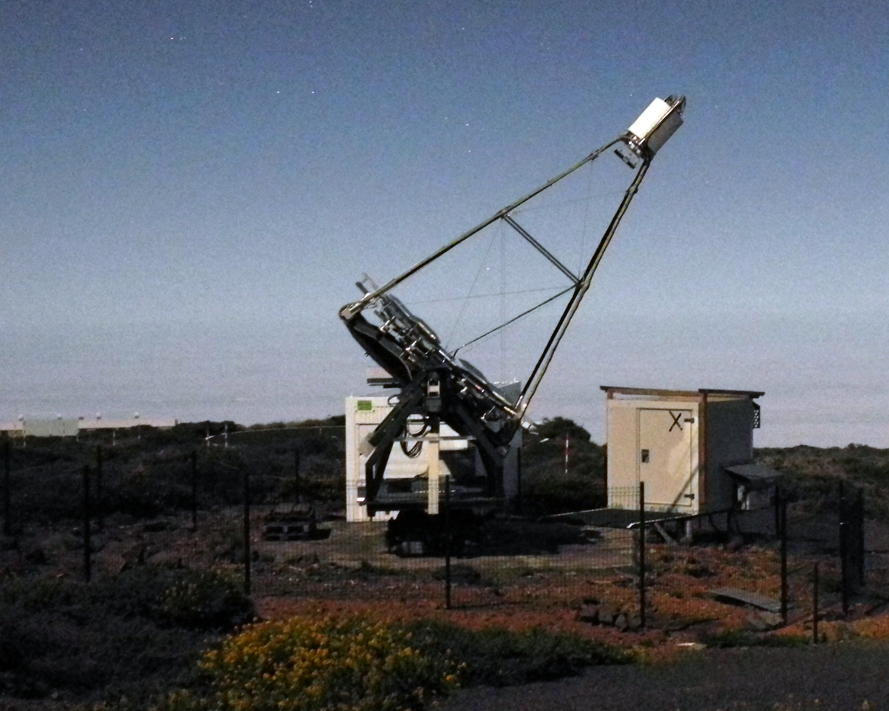
Figure 1: Picture of the FACT telescope during observations at night. In the background, the white container hosting the computing system, the bias power sully and the drive system is visible. Courtesy of D. Dorner.

For the first time in Cherenkov astronomy, photo multiplier tubes (PMT) for photo detection have been replaced by more modern silicon based photo sensors. The First G-APD Cherenkov Telescope (FACT) has implemented a focal plane using 1440 Hamamatsu MPPC S10362-33-050C sensors for photo detection. A picture of the telescope can be seen in Fig. 1. A detailed description of its hardware and software is given in the FACT design report [1].

Apart from the use of recent technology for photo detection, the FACT project aims towards long-term monitoring of the brightest known blazars at TeV energies. Due to the natural gap in observations, which arises from bright moon light when operation with photo multiplier tubes is hardly possible with standard settings, and the busy schedule of existing high performance instruments, the existing sampling density is comparably low in the order of a few minutes every few days. Therefore, the aims is a high duty cycle instrument with the best possible data taking efficiency and observations during strong moon light, so that several hours per night and source can be achieved and the gap around full moon can be filled.

Data taking efficiency and the results of almost two years of successful monitoring of Markarian 421 and Markarian 501 are presented at the end of the paper. In the following, the use of Geiger-mode avalanche photo sensors in the camera are discussed in more details and results from stability measurements are presented.

I-A Application of G-APDs

In Cherenkov astronomy, photo sensors are used to detect Cherenkov light emitted by particle cascades in the atmosphere. The image of these particle showers is then used to reconstruct the properties of the primary particles such as particle type, energy and origin.

To detect these nano-second short light-flashes consisting of a few tens to hundreds of photons, sensitive and fast photo sensors are needed. Since its beginning, Cherenkov astronomy has used photo multiplier tubes for photo detection, but for several years silicon based photo sensors are on the market as well. During the past years, Geiger-mode avalanche photo diodes (G-APD) became powerful and inexpensive enough to replace photo multiplier tubes in Cherenkov astronomy.

Each sensor applied in the FACT camera consists of 3600 single Geiger-mode avalanche photo diodes (cells), 50 $\mu$m x 50 $\mu$m each. Since the cells are operated above their breakdown voltage, the so-called Geiger-mode, each detected photon triggers a complete discharge of a single cell. The resulting pulse is comparable in amplitude and shape for all cells. Due to the high precision of the production, the fluctuations from cell to cell are small.

Devices currently on the market achieve photo detection efficiencies comparable to the best available PMTs, and improved photo detection efficiency is expected for the next generation.

As compared to PMTs, silicon based photo sensors are easier to handle due to their lower bias voltage in the order of 100 V or below, they are mechanically more robust, and they are insensitive to magnetic fields. Apart from their high future potential, their main advantage in Cherenkov astronomy is their robustness against bright light which allows operation under bright moon light conditions.

As a drawback, G-APDs encounter a high dark count rate, so-called optical crosstalk and a comparably high afterpulse probability.

The dark count rate of the applied sensors is in the order of 1 MHz to 9 MHz for typical operation temperatures between 0 °C to 30 °C. At the same time, the rate of detected photons from the diffuse night sky background is in the order of 30 MHz to 50 MHz even during the darkest nights. Consequently, the dark count rate of the sensor is negligible.

I-B Dark count rate, optical crosstalk and afterpulses

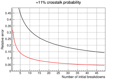
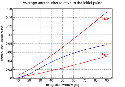
Figure 2: Left: The figure shows the relative error introduced on average by optical crosstalk (red) and its statistical error (black) on the signal as a function of the number of initial breakdowns considering a crosstalk probability of 11%. In both cases, the error on a single event can be significantly larger, but on average the statistical error dominates considerably. Right: The figure shows the additional contribution from afterpulses (blue) as a fraction of the unbiased pulse as a function of the applied pulse integration window starting pulse integration at the half height leading edge compared to the contribution from optical crosstalk (red). While the relative contribution by afterpulses does not depend on the initial number of breakdowns, the relative contribution from optical crosstalk decreases with an increasing number of breakdowns. While the contribution from afterpulses in single events can reach 100% the number of biased events is so small, that the average contribution for integration windows of less than 40 ns is below 4%.

The so-called optical crosstalk is the probability that the discharge of a G-APD cell will indirectly trigger at least one other cell due to photons potentially emitted during the breakdown. While this effect is significant for signals in the order of one, for larger signals it just increases the amplitude and its fluctuation statistically. Figure 2 shows the relative error introduced from crosstalk compared to the statistical error. Since the signals of Cherenkov showers are comprised of a number of photons large compared to one, and have an intrinsic fluctuation of the order of a few percent, optical crosstalk needs to be considered quantitatively in the shower reconstruction, but has no significant effect on the quality.

Afterpulses in G-APDs originate from trapped charges released with a short delay after the initial pulse. Their probability is exponentially decreasing with a time scale in the order of the decay time of the pulse, see [2]. Figure 2 shows the influence of afterpulses as a function of the integration window. Although their total probability in the order of 10% to 20% is high compared with PMTs, they usually occur within the timescale of the initial pulse. The exponential decrease of the probability ensures that afterpulses induced by coincident signals in several cells or sensors are not released synchronously. Therefore, afterpulses in G-APDs can not fake trigger signals in contrast to afterpulses in PMTs. In addition, due to the partial discharge of the cell after the initial pulse, the amplitude of early afterpulses is highly decreased. Generally, their absolute amplitude, i.e. falling edge plus afterpulse, does not exceed the amplitude of the initial pulse. In the pulse extraction algorithm, their influence can be suppressed strongly, if the integration range is limited to a short interval around the peak of the initial pulse.

I-C Breakdown voltage

The main challenge in the application of G-APDs in an experiment exposed to changing environmental conditions is the dependence of their breakdown voltage from the temperature and the voltage drop induced by high currents.

Cherenkov telescopes are exposed to natural temperature changes during the night. Since the breakdown voltage of the G-APDs in use is temperature dependent ($\approx$55 mV/K), the gain will follow the temperature, if the voltage is not adjusted accordingly.

In addition, each sensor has a network of serial resistors. When the moon rises during the night, more breakdowns take place due to the increased photon flux and induce a higher current in the resistors. The voltage drop induced at the serial resistors is enough to significantly decrease the gain of the sensor. Therefore, this voltage drop must be determined and the applied voltage has to be adjusted accordingly.

In the following, the calibration and adjustment procedure applied in the FACT camera is presented and discussed.

II Bias voltage calibration

The camera contains a total of 1440 photo sensors and 320 bias voltage channels. Four respectively five sensors are combined into a single bias channel at a time. To avoid influences of different operation voltages of the sensors combined into a single channel, the sensors in each channel are ordered together according to the operation voltage provided by the manufacturer. The operation voltage is provided with a precision of 0.01 V which corresponds to a precision of $\approx$1% in gain at the operation voltage.

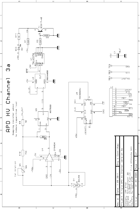
Figure 8: Schematics of the circuit which provides the bias power for the G-APDs. It is controlled by an digital-to-analog converter and the drawn current is measured by an analog-to-digital converter.

The schematics for a reference channel is shown in Fig. 8 at the end of the paper. The circuit is driven by a current supplying 12 bit digital-to-analog converter (DAC) with a maximum current output of 1 mA. Its output voltage is amplified by an op-amp (OPA 454) which is operated in a programmable voltage source configuration, c.f. its datasheet. A calibration resistor in the feedback loop allows to adjust the voltage output of each channel. A measurement circuit with a 12 bit analog-to-digital converter (ADC) measures the current drawn by both, the feedback loop and the attached sensors. The voltage output and camera input have damping resistors, 1 k$\Omega$ each, to avoid oscillations by the capacitance of the cable. Each sensor has its own serial resistor (3.9 k$\Omega$).

With a nominal calibration resistor of 90 k$\Omega$, the voltage output realized by the circuit for the full range of the DAC is between 0 V and 90 V in steps of 22 mV. The current can be measured with a precision of 1.2 $\mu$A in a range between 0 A and 5 mA.

In an ideal circuit with an ideal op-amp, no further calibration is necessary. A real circuit must be calibrated to correct for the non-ideal behavior of the op-amp and the limited accuracy with which the total resistances are known. This is necessary to achieve the maximum possible precision in the absolute voltage output of 22 mV at roughly 70 V corresponding to about 0.3%. To calibrate the circuit, the voltage output at U_OUT and the corresponding feedback value from the ADC are measured as a function of the DAC setting. This measurement takes place well below the breakdown voltage of the G-APD to ensure that the sensors do not draw any current through U_OUT, neither in avalanche mode nor in Geiger-mode.

II-A Correcting the voltage drop

The calibration of the voltage output versus DAC setting is mainly necessary due to the non-ideal behavior of the op-amp. Since a non ideal op-amp usually draws current on its input, the measured current at the ADC is not exactly identical with the current provided by the DAC and needs to be calibrated as well.

Above 50 V, the behavior of the circuit can be considered linear within the precision of the DAC setting, so that only slope and offset need to be calibrated.

The output voltage $U_{out}$ at U_OUT can be expressed as a function of the DAC setting as

$$U_{out}=u+r\cdot I_{dac}$$

with the calibration constants $u$ and $r$ determined by calibration measurements.

With the ADC, the voltage drop at $R_{8}$ is measured precisely, corresponding to the current $R_{8}$, and below the breakdown voltage of the G-APDs when no current flows through $R_{4}$ also at $R_{9}$ and $R_{10}$. Therefore, it gives the current $I_{9}$ as a function of the DAC setting assuming that the imprecisions of $R_{8}$ and the imprecision of the measurement curcuit can be neglected against the deviations of $I_{9}$ from the output current of the DAC:

$$I_{9}=i+c\cdot I_{dac}$$

with the calibration constants $i$ and $c$ determined by the calibration measurements.

Below the breakdown voltage, the voltage at the sensors is then equal to the calibrated output voltage U_OUT. If the breakdown voltage is exceeded, an additional current will flow through U_OUT and the 100 $\Omega$ measurement resistor induces an additional voltage drop which has to be taken into account.

The current leaking through U_OUT can then be calculated as the difference between the current $I_{8}$, equal to the measured current $I_{adc}$, and the current $I_{9}$ through $R_{9}$ and $R_{1}0$:

$$I_{out}=I_{8}-I_{9}=I_{adc}-I_{9}=I_{adc}-(i+c\cdot I_{dac})$$

The voltage drop at the resistors $R_{4}$, $R_{5}$ and $R_{n}$ for $N$ parallel sensors is calculated by

$$U_{drp}=(1\,\mbox{k}\Omega+1\,\mbox{k}\Omega+\frac{3.9\,\mbox{k}\Omega}{N})\cdot I_{out}.$$

The resistor $R_{5}$ is an additional serial resistor of 1 k$\Omega$ in each bias channel on the camera side, while $R_{n}$ are resistors of 3.9 k$\Omega$ within each individual sensor branch.

II-B Correcting the change of operation temperature

In addition to the voltage drop, an intrinsic feature of each resistor network, the change in operation voltage of the G-APDs by temperature variations, has to be considered. Therefore, 31 temperature sensors were homogeneously distributed on the sensor plate. Their values are read out once every 15 s and inter- respectively extrapolated linearly to get an estimate of the temperature of each bias patch. The difference between the minimum and maximum temperature in the camera never exceeds 4 K. To correct for the measured temperature, the change on operation voltage $\Delta U$ is calculated as

$$\Delta U=(25\,^{\circ}\mbox{C}-T)\cdot t$$

for each patch separately at a patch temperature $T$ and a temperature coefficient $t$. How the temperature for each patch is determined is described in the next section.

The nominal voltage setting $U_{set}$ is then derived as the manufacturer given operation voltage $U_{op}$, the temperature correction $\Delta U$ and the voltage drop $U_{drp}$ at the nominal set-point:

$$U_{set}=U_{op}+\Delta U(T)+U_{drp}(U_{set}).$$

III Temperature measurement

To achieve a reasonable precision, the average temperature of the sensors supplied by a single bias voltage channel has to be known. Therefore, the temperatures measured by the temperature sensors needs to be inter- respectively extrapolated. Since three of them do not show any signal, 28 are available in total. It was planned to repair the remaining three sensors, but since their access is very diffcult and the camera has to be unmounted, the effort has never been carried out because no significant improvement is expected.

For interpolation, a so-called Delaunay triangulation is calculated. A Delaunay triangulation connects each set of three points from a set of points such that no other point is inside the circumcircle of the three points. Delaunay triangulations maximize the minimum angle of all the angles of the triangles in the triangulation and therefore avoid skinny triangles.

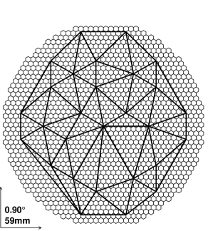
Figure 3: This figure shows the Delaunay triangulation for the working temperature sensors in the camera. Each intersection point corresponds to one sensor.

The Delaunay-triangulation for the set of the 28 working sensors has been calculated. The triangulation is shown in Figure 3 where the cross points of the edges of the triangles correspond to the sensor positions.

For each point inside any of the triangles, the temperature can now be interpolated linearly. For each point outside the border of the Delaunay triangulation, an extrapolation algorithm is applied. To get a reasonable and continuous extrapolations, the following algorithm is applied: If the point does not lay within a triangle, choose the set of three points for which it lays within their circumcirle. If no such circle is available, choose the triangle with the closest circle center. The extrapolation is then done linear for the set of three points. It should be mentioned, that this algorithm gives comparable good results very close to the border of the Delaunay-triangulation, but is not suited for points further away as any extrapolation algorithm.

In principle, more complex interpolation algorithms, e.g. natural neighbor interpolation or dimensional splines, could be applied. While the maximum temperature difference in the camera might reach values of 4 ° just after sunset, the typical maximum temperature difference in the camera is not more than 1.5 °C. Even for the most extreme cases, this yields a maximum temperature difference of 1 °C in a single triangle corresponding to 5% in gain. Therefore, a linear interpolation can be considered precise enough.

IV Results

To measure the stability of the system, two main methods are available. The first method extracts the gain from the dark count spectrum, the second uses an external light pulser as signal source. The advantage using the dark count spectrum, is the availability of a very precise and unbiased method to measure the gain directly. Evaluating a spectrum of random signals induced from the diffuse night-sky background under dark night condition is possible as well, but leads to less stable results. Extracting single pulses from data taken with additional background light is extremely chellenge. This limitation can be overcome using a stable external light source which produces an amplitude well above the night-sky light level. In contrast to the dark count spectrum, this method is biased by the transmission of the light-collecting cones, the photo detection efficiency of the sensors and the stability of the light source itself. In this context, the dark count spectrum is well suited to extract the dependency of the gain on the sensor temperature, while light-pulser measurements provide information about the dependency on the background light-level or the resulting current.

A third method is to use the physics triggered data itself, so called ratescans, for a qualitative estimation of the stability. Details can be found in [3].

More about that can be found as well in [4].

IV-A Temperature dependence

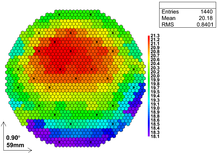
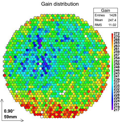
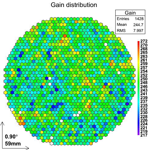
Figure 4: The left camera display shows interpolated temperatures for all pixels (the same value for all pixels connected to the same bias channel) in degree Celsius for data taken just after sunset. The central camera display shows the gain in arbitrary units extracted for each pixel, if the applied voltage of all pixels is corrected for the average temperature of all 28 sensors instead of the individual patch temperature. The variance is 4.5%. The right camera display shows the gain extracted, if individual patch-wise corrections for the operation voltage are applied. The variance has decreased to 3.3%. Both displays feature identical color scales.

Figure 4 shows a typical temperature distribution, directly after sunset with a maximum temperature difference of 3.2 °C, a gain distribution in which for all bias channels an average correction is applied and a gain distribution in which a per channel correction is applied. Both measurements took place directly after each other, and the gain was extracted from a dark count spectrum taken with closed lid. It can be seen that the distribution of gains without channel-wise correction depends on the temperatures in the camera as expected. If the temperature correction is applied per bias channel, an improvement of the width of the distribution from 4.5% to 3.3% is visible.

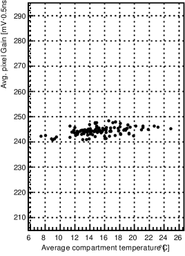
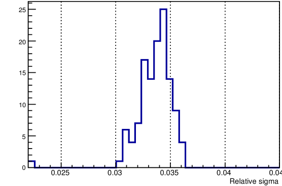
Figure 5: The left figure shows the average gain extracted from 110 measurements in arbitrary units versus the corresponding average sensor temperature in degree Celsius. A small remaining dependence is visible, most probably due to a non-ideal temperature coefficient. The spread of the distribution is less than 1%. The right figure shows the distribution of the corresponding variance relative to the average. The typical spread of gain values in the camera is 3.4% on average.

In total, 110 such distributions have been measured during two months with a temperature range between 6 °C and 24 °C with several measurements each night. Figure 5 shows the average gain of all pixels versus the average temperature of the 28 temperature sensors. Although the variance of the distribution is less than 1%, still a remaining dependence on temperature is visible. It can be attributed to a non-ideal temperature coefficient. Since the remaining temperature difference is in the order of less than 1 mV a large statistics is needed to reach that precision. A camera with more than 1400 channels is ideally suited for that. The shown data has been used to apply a correction on the coefficient. Currently, new data is recorded to investigate the expected improvement. In addition to the average dependency on temperature, the gain spread in the camera can be investigated. Figure 5 shows the distribution of variances of the measurements for the gain distributions. It is independent of the temperature and has an average value of 3.4%.

For all those measurements, typical currents per sensor are in the order of 1 $\mu$A or below, which is close to the resolution of the current readout and the corresponding voltage drop is within the resolution of the voltage setting. If the lid is opened, this does not apply anymore and a correction for the induced voltage drop has to be introduced.

IV-B Current dependency

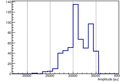
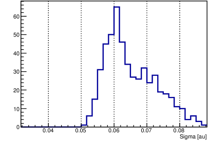
Figure 6: The left figure shows the average amplitude in arbitrary units extracted from several light-pulser runs, the right figure the distribution of the spread in the camera relative to the average. The variance of the average is below 10%, the typical spread in the camera is around 6%. This includes the inhomogeneity of the light yield from the light pulser, the fluctuation in its light yield and a small remaining temperature dependance of its light yield.

If the camera lid is open, the camera is exposed to the photon flux from the diffuse night-sky background light resulting in typical currents per sensor in the order of 5 $\mu$A to 10 $\mu$A during dark night. At full moon nights this can reach currents of 200 $\mu$A per sensor or more.

To measure the dependency on background light level expressed as current per sensor, dedicated runs of light-pulser data are taken about every 20 minutes during the night. The distribution of the average amplitude seen in the camera and its variance are shown in Figure 6. The variance of the distribution on averages is below 10%, the mean of the distribution on the variances is roughly 6.5%. It should be mentioned that the light distribution of the pulser has a systematic uncertainty of a few percent and a remaining temperature dependence of its amplitude also in the order of a few percent is known.

IV-C Data taking efficiency and automation

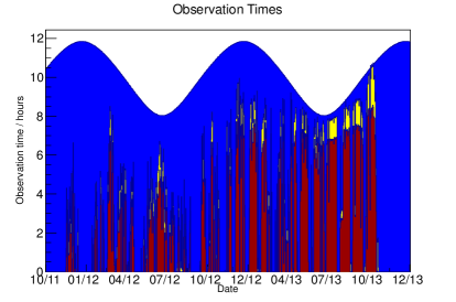
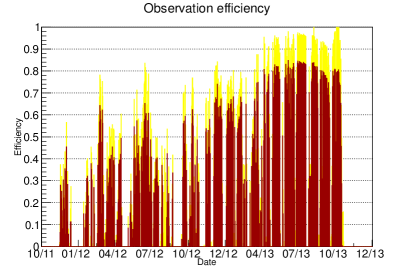
Figure 7: The left figure shows the observation total time of data taken per night (yellow) and the total time of physics triggered data taken (red). The difference is the amount of calibration data recorded. As a reference, the total available data taking time is shown (astronomical twilight) in blue. The right plot shows the corresponding efficiency normalized to the available twilight time. Roughly since April 2013, data taking is fully automatic which is clearly visible in the data taking efficiency. The regular gaps originate from full moon days during which the telescope cannot be operated due to safety reasons. Other downtime is usually related with bad weather.

To achieve the goal of long-term monitoring of the brightest known TeV blazars with a high duty cycle, the system has been fully automated. Although improvements are continuously on-going, the system is now operated with a pre-defined schedule usually without interruption from the beginning to the end of the night without manual interaction. The main reasons for down time are now mainly bad weather conditions and too bright moon light. Since the light of the moon and thus currents are disproportionately hight around full moon, for safety reasons currently an operation limit is imposed on the currents. In addition, no shift crew is available on the site of the close-by MAGIC telescope, which prevents remote operation due to an agreement with the MAGIC collaboration for safety reasons. Apart from these unavoidable constrains, data taking efficiency is only limited by the high amount of calibration data still taken to get a good understanding of the system in all possible conditions. The least possible amount of time is lost due to the configuration of the system at the beginning of each run or re-pointing of the telescope. Starting a run takes about one second, while re-positioning takes a few seconds for the movement and a few seconds for the voltage to become stable again after that. In total, usually less than 40 s are lost for each 20 min block of data-taking which corresponds to an efficiency of about 97% (including calibration data). Figure 7 shows the total data taking per night, the time of astronomical twilight. Super-imposed is the total time the system operated and the time physics data was recorded. The second plot shows the corresponding efficiencies. It can be seen that since a few months, the operation efficiency during the night usually exceeds 95% and the data taking efficiency for physics triggered data exceeds 80%. Data taking can be monitored online at http://www.fact-project.org/smartfact. In addition, work to operate the telescope fully robotically are in-going, c.f. [5].

IV-D Monitoring

Due to automation, the resulting high data taking efficiency results in a dense and complete sampling of the monitored sources. In [6] the excess rates as measured from the blazars Markarian 421 and Markarian 501 between May 2012 and July 2013 are shown. First results were presented in [7]. The typical observation time is in the order of a few hours per night. Observations are typically carried out up to a moon disk of 85% to 90%. In total 167 hours of data have been collected for Markarian 421 and 242 hours for Markarian 501. Since the data taking procedure was optimized and data taking is fully automatic, sampling density has significantly improved. The results of the analysis are immediately publicly available online at http://www.fact-project.org/monitoring, typically with a delay not less than 20 min. For data taking and online analysis in total four to five cores are loaded on average in two PCs.

V Conclusions

The First G-APD Cherenkov telescope has proven the possibility to apply Geiger-mode avalanche photo diodes in Cherenkov astronomy for photo detection. Their gain has been shown to be independent of the temperature within 1% in a temperature range between 0 °C to 30 °C and independent from the night-sky background light level within at least 6.5%. The gain distribution of the 1440 pixels is not wider than 3.4% with a closed lid and 10% with open lid, which includes the inhomogeneity of the light-pulser’s light distribution used for the measurement. These stability has been achieved independent of any external calibration device. The external light-pulser has only be used to measure the G-APD properties. Currently, more calibration measurements are taken to improve these results further.

With a high level of automation, the fully remote controlled telescope, achieves a data taking efficiency of typical 85% and more than 95% if calibration measurement are included. Configuration and re-positioning times are less than 5% in total.

Recently, it was proven that observations even close to the full moon are possible, c.f. [8].

Monitoring of the two brightest known blazars is carried out successfully since two years and the excess rates of the past 1.5 years have been present including a couple of minor and major flares. The results from an online analysis are available online immediately after data taking.

References

- [1] H. Anderhub et al. (FACT Collaboration) 2013, JINST 8 P06008 [arXiv:1304.1710].
- [2] A. Du and F. Retiere, NIM A 596, 3, 396.
- [3] D. Hildebrand et al. (FACT Collaboration) 2013, in Proc. of the \nth33 Int. Cosmic Ray Conf., ID 709.
- [4] T. Bretz et al. (FACT Collaboration) 2013, in Proc. of the \nth33 Int. Cosmic Ray Conf., ID 683.
- [5] A. Biland et al. (FACT Collaboration) 2013, in Proc. of the \nth33 Int. Cosmic Ray Conf., ID 708.
- [6] D. Dorner et al. (FACT Collaboration) 2013, in Proc. of the \nth33 Int. Cosmic Ray Conf., ID 686.
- [7] T. Bretz et al. (FACT Collaboration) 2012, AIPC 1505, 773.
- [8] M. Knoetig et al. (FACT Collaboration) 2013, in Proc. of the \nth33 Int. Cosmic Ray Conf., ID 695.