Cosmology from weak lensing of CMB

Abstract

The weak lensing effect on the cosmic microwave background (CMB) induces distortions in spatial pattern of CMB anisotropies, and statistical properties of CMB anisotropies become a weakly non-Gaussian field. We first summarize the weak lensing effect on the CMB (CMB lensing) in the presence of scalar, vector and tensor perturbations. Then we focus on the lensing effect on CMB statistics and methods to estimate deflection angles and their power spectrum. We end by summarizing recent observational progress and future prospect.

1 Introduction

The path of CMB photons emitted from the last scattering surface of CMB is deflected by gravitational potential of the large-scale structure with typically a few arc-minute deflection. This leads to the distortion in spatial pattern of observed CMB anisotropies. Among various cosmological observations, a measurement of weak lensing signals in CMB maps is a direct probe of intervening gravitational fields along a line of sight, and is considered as one of the most powerful probes of fundamental issues in cosmology and physics in the near future.

Most of the pioneering work in CMB lensing focused on how the lensing effect modifies the two-point statistics of CMB temperature anisotropies (e.g., Blanchard:1987AA ; Sasaki:1989 ; Tomita:1989 ; Fukushige:1994 ; Seljak:1995ve and Refs therein). An accurate calculation of lensing effect on the angular power spectrum by Ref. Seljak:1995ve showed that the acoustic scale imprinted in temperature is slightly smoothed and the small scale temperature fluctuations are enhanced by transferring large scale power to small scale. On the other hand, Refs. Bernardeau:1996aa ; Zaldarriaga:2000ud showed that the lensing effect also modifies the statistics of CMB anisotropies and generates non-Gaussian signatures in the observed CMB anisotropies. A more interesting and important effect for future studies of CMB lensing is that the gravitational lensing generates B-mode polarization converted from E-mode polarization Zaldarriaga:1998ar .

Although the theoretical framework of CMB lensing has been established a decade ago, a significant observational progress has been made only recently. The lensing effect on CMB temperature and polarization anisotropies as well as the gravitational lensing potential are now measured with both ground-based and satellite experiments (e.g., Reichardt:2008ay ; Das:2011ak ; Hanson:2013daa and see Sec. 5 for details), requiring studies of more practical issues which are now rapidly developing. The measured lensing signals are already used for some specific issues in cosmology, e.g., dark energy Sherwin:2011gv ; vanEngelen:2012va ; Ade:2013tyw ; Ade:2013zuv , dark matter Wilkinson:2013kia , cosmic strings Namikawa:2013wda , and primordial non-Gaussianity Giannantonio:2013kqa . Although statistical significance of the current detections of lensing signals is not so high compared to other cosmological probes, the lensing signals obtained from upcoming and next generation experiments will have enough potential to probe the following fundamental issues:

• Dark energy, Dark matter and Massive neutrinos: The theoretical understanding of the nature of the dark energy is still limited, and the cosmological observations are the only way to reveal the dynamical properties of the dark energy. On the other hand, determination of the neutrino mass is one of the most important subjects in elementary particle physics, and is the key to understand the physics beyond the standard model of particle physics. The properties of the dark energy, specific models of dark matter, and mass of neutrinos affect the evolution of gravitational potential, and thus the signals of weak lensing.

• Gravitational waves, Cosmic strings and Magnetic fields: A measurement of the curl mode of deflection angles is also interesting for cosmology (see Sec. 2). The curl-mode deflection angles are produced by the vector and tensor metric perturbations, but not by the scalar perturbations. That is, the non-vanishing curl-mode signal is a smoking gun of the non-scalar metric perturbations which can be sourced by gravitational waves Cooray:2005hm ; Namikawa:2011cs and cosmic strings Namikawa:2011cs ; Yamauchi:2012bc ; Yamauchi:2013fra which may give clues about the mechanism of inflationary scenario at the early universe and implications for high-energy physics. The magnetic fields at cosmological scales would also be probed with the curl mode which will be explored in our future work.

In addition, the study of CMB lensing has implications for detecting the signature of the primordial gravitational waves, since the amplitude of CMB B-mode polarization generated from primordial gravitational waves is smaller than that from lensing if the tensor-to-scalar ratio is very small Knox:2002pe . In order to enhance sensitivity to the primordial B-mode polarization, subtraction of the lensed B-mode would become important Verde:2005ff ; Smith:2008an ; Smith:2010gu ; Abazajian:2013vfg . Similarly, since the lensing induces the non-Gaussian signatures in CMB anisotropies and non-zero off-diagonal elements in the covariance matrix, the lensing effect would be a possible confusing source in estimating the primordial non-Gaussianity or testing the statistical isotropy. For this reason, precise and accurate estimations of lensing effect on CMB maps are required.

As the measurements of lensing effect become more precise, the studies of CMB lensing should focus more on practical issues rather than on purely theoretical issues. For example, reconstruction of gravitational potential, which is mainly used for analysis of CMB lensing, is based on the assumption that the primordial CMB anisotropies are statistically isotropic. There are, however, several possible sources to generate mode couplings in the anisotropies such as the mask of Galactic emission and point sources Carvalho:2010rz ; BenoitLevy:2013bc , inhomogeneous noise, Hanson:2009dr , beam asymmetry Hanson:2010gu , and so on. These contaminations potentially lead to a significant bias in the estimation of lensing potentials. For accurate cosmology with future observations, methods for mitigating all these biases are needed.

This paper is organized as follows. In Sec. 2, we formulate the weak gravitational lensing in the presence of scalar, vector and tensor metric perturbations, and see how the lensing signals depend on cosmological sources. In Sec. 3, we show how the lensing effect modifies the statistics of the observed CMB anisotropies. In Sec. 4, we discuss the method for estimating the deflection angles and their power spectrum. Sec. 5 is devoted to summary of recent observational status and future prospect.

2 Weak gravitational lensing from scalar, vector and tensor perturbations

Consider a photon emitted from the last scattering surface of CMB, which passes through gravitational fields before reaching us. The geodesic of the photon is perturbed by the gravitational lensing, and the photon is observed in a different direction from the original direction. The difference between observed and original directions is called the deflection angle which provides information on the anisotropies of projected gravitational fields integrated from the last scattering surface to the observer. In this section, we review how the deflection angle is related to the gravitational fields and how its power spectrum depends on properties of several cosmological sources such as the dark energy, massive neutrinos and cosmic strings.

2.1 Gradient and curl modes of deflection angle

The expression for the deflection angle with the metric perturbations is obtained by solving the photon geodesic in a perturbed universe. Let us consider the line element given by

$${\rm d}s^{2}=a^{2}(\eta)(\bar{g}_{\mu\nu}+\delta g_{\mu\nu}){\rm d}x^{\mu}{\rm d}x^{\nu}\,,$$ (1)

where $a$ is the scale factor in a homogeneous and isotropic universe, $\bar{g}_{\mu\nu}$ is the background unperturbed metric and $\delta g_{\mu\nu}$ is the small metric perturbations. Here we assume that the unperturbed metric is described by the flat Friedman-Lemaître-Robertson-Walker metric:

$$\bar{g}_{\mu\nu}{\rm d}x^{\mu}{\rm d}x^{\nu}=-{\rm d}\eta^{2}+\bar{\gamma}_{ij}{\rm d}x^{i}{\rm d}x^{j}=-{\rm d}\eta^{2}+{\rm d}\chi^{2}+\chi^{2}\omega_{ab}{\rm d}\theta^{a}{\rm d}\theta^{b}\,,$$ (2)

with $\omega_{ab}{\rm d}\theta^{a}{\rm d}\theta^{b}={\rm d}\theta^{2}+\sin^{2}\theta{\rm d}\varphi^{2}$ denoting the metric on the unit sphere. In the conformal Newton gauge, the metric perturbations are described as

$$\delta g_{00} =-2\Phi\,, \delta g_{0i} =-\sigma_{i}\,, \delta g_{ij} =2\Psi\bar{\gamma}_{ij}+h_{ij}\,,$$ (3)

where the quantities, $\Phi$ and $\Psi$, are the scalar components, $\sigma_{i}$ is the divergence-free vector component ($\sigma_{i}{}^{|i}=0$), and $h_{ij}$ is the transverse-traceless tensor component ($h_{ij}{}^{|i}=0$, and $h^{i}{}_{i}=0$). The vertical bar ($|$) denotes the covariant derivative with respect to the background three-dimensional metric, $\bar{\gamma}_{ij}$.

To define the deflection angle, let us consider null geodesics in the background and perturbed spacetime, $\bar{x}^{\mu}$ and $x^{\mu}$. Since the photon path is not deflected in the background spacetime, the unperturbed path can be parametrized as $\bar{x}^{\mu}=(\eta_{0}-\chi,\chi\widehat{n}^{i})$. Here the quantity $\eta_{0}$ denotes the conformal time today and $\widehat{n}^{i}$ is the unit vector describing the observed direction of photon. Assuming a static observer, we define the deflection angle by projecting the angular components of the deviation vector $x^{\mu}-\bar{x}^{\mu}$ on the sphere Yamauchi:2013fra :

$$d^{a}\equiv\frac{[x^{i}(\chi_{\rm s})-\bar{x}^{i}(\chi_{\rm s})]e_{i}{}^{a}}{\chi_{\rm s}}-\theta^{a}_{O}\,,$$ (4)

where the subscript $a$ means the angular components, $\theta$ and $\varphi$. The three-dimensional vectors, $e_{i}{}^{a}$, are the basis vectors orthogonal to $\widehat{n}^{i}$, the quantity, $\chi_{\rm s}$, is the conformal distance between the observer and the last scattering surface of CMB, and $\theta^{a}_{O}$ is the angular coordinate at the observer. Since the deflection angle has two degrees of freedom, we decompose the deflection angle into two components by parity symmetry as Stebbins:1996wx ; Hirata:2003ka ; Cooray:2005hm ; Namikawa:2011cs

$$d^{a}=\phi^{:a}+\epsilon^{a}{}_{b}\varpi^{:b}\,,$$ (5)

where $(:)$ is the covariant derivative on the unit sphere, and $\epsilon^{a}{}_{b}$ denotes the two-dimensional Levi-Civita symbol. Hereafter, we call the first and second terms in the right-hand side of Eq. (5) gradient and curl modes, respectively.

The deviation vector is obtained from the geodesic equation in the perturbed spacetime, and the resultant expressions for the gradient and curl modes are given by Yamauchi:2013fra

$$\bm{\nabla}^{2}\phi=d^{a}{}_{:a}={\int_{0}^{\chi_{\rm s}}\!\!\frac{\,{\rm d}\chi\,}{\chi}\,}\biggl{\{}\frac{\chi_{\rm s}-\chi}{\chi_{\rm s}}\bm{\nabla}^{2}[2\psi+\mathcal{A}]-\mathcal{B}^{a}{}_{:a}\biggr{\}}\,,$$ (6)

$$\bm{\nabla}^{2}\varpi=d^{a}{}_{:b}\,\epsilon^{b}{}_{a}=-{\int_{0}^{\chi_{\rm s}}\!\!\frac{\,{\rm d}\chi\,}{\chi}\,}\mathcal{B}^{a}{}_{:b}\,\epsilon^{b}{}_{a}\,.$$ (7)

Here $\bm{\nabla}^{2}$ is the Laplacian operator on the unit sphere, $\psi=(\Phi-\Psi)/2$, and we define the quantities generated by non-scalar perturbations:

$$\mathcal{A}=\sigma_{i}\widehat{n}^{i}+h_{ij}\widehat{n}^{i}\widehat{n}^{j}\,,\ \ \ \mathcal{B}_{a}=\sigma_{i}e^{i}_{a}-2h_{ij}e^{i}_{a}\widehat{n}^{j}\,.$$ (8)

In Eqs. (6) and (7), the integral at the right-hand-side is evaluated along the unperturbed light path, usually referred to as the Born approximation (see e.g. Ref. Cooray:2002mj for the correction terms). The radial displacement (or the time delay) is also discussed in Ref. Hu:2001yq , but is a negligible effect on statistical observables.

Eq. (7) shows that the curl mode of the deflection angle vanishes if we consider the scalar perturbations alone, but it is produced by the vector and/or tensor components. Also, beyond the liner perturbation, the curl mode is generated, e.g., by the second order of the density perturbations Hirata:2003ka ; Sarkar:2008ii .

It is also worth noting about the relation between the deflection angle and the elements of the Jacobi matrix which is defined as the mapping between a source and an image plane. The relation between the deflection angle and the Jacobi matrix is obtained by solving the geodesic deviation equation. Denoting the symmetric-traceless part of the Jacobi matrix divided by $\chi_{\mathrm{s}}$ as $\gamma_{ab}$ (shear components), the relation becomes Schmidt:2012nw ; Yamauchi:2013fra

$$\gamma_{ab}=d_{\langle a:b\rangle}+\frac{1}{2}[h_{\langle ab\rangle}]_{0}^{\chi_{s}}\,,$$ (9)

where, for any quantity, $X_{\langle ab\rangle}=(X_{ab}+X_{ba}-X^{c}{}_{c}\omega_{ab})/2$. The last term arises in the presence of tensor perturbations as a difference of coordinate system perturbed by the metric at observer and source position Dodelson:2003bv .

2.2 Angular power spectrum of gradient and curl modes

Once we measure the deflection angle, one of the useful quantities in cosmology is the angular power spectrum of fluctuations, rather than the fluctuations themselves. Here we turn to discuss the angular power spectrum of the gradient and curl modes, based on Eqs. (6) and (7). To see how the observable depends on properties of the cosmological sources, we also show the relation between the angular power spectrum and the power spectrum of metric perturbations.

2.2.1 Scalar perturbations alone

Let us first consider the case in the presence of scalar perturbations alone, since it helps our understanding of derivation in the presence of the non-scalar perturbations.

The fluctuations of gravitational potential are decomposed into Fourier modes with the scalar-mode function $Q^{(0)}(\bm{x},\bm{k})=\hskip 1.00006pt{\rm e}^{-{\rm i}\hskip 0.35002pt\bm{k}\cdot\bm{x}}$ as

$$\psi(\bm{x},\eta) ={\int\!\!\frac{\,{\rm d}^{3}\bm{k}\,}{(2\pi)^{3}}\,}\psi_{\bm{k}}(\eta)Q^{(0)}(\bm{x},\bm{k})\,.$$ (10)

Substituting the above equation into Eq. (6), we obtain

$$\bm{\nabla}^{2}\phi=2{\int_{0}^{\chi_{\rm s}}\!\!\,{\rm d}\chi\,\,}\frac{\chi_{\rm s}-\chi}{\chi_{\rm s}\chi}{\int\!\!\frac{\,{\rm d}^{3}\bm{k}\,}{(2\pi)^{3}}\,}\psi_{\bm{k}}(\eta)\bm{\nabla}^{2}Q^{(0)}(\chi\hat{\bm{n}},\bm{k})\,.$$ (11)

The angular power spectrum is defined as

$$\delta_{\ell\ell^{\prime}}\delta_{mm^{\prime}}C_{\ell}^{\phi\phi}=\langle\phi_{\ell m}\phi_{\ell^{\prime}m^{\prime}}^{*}\rangle\,,$$ (12)

where the quantity $\phi_{\ell m}$ is the spherical harmonic coefficients of the gradient mode and is defined with the spin-$0$ spherical harmonics $Y_{\ell m}(\hat{\bm{n}})$ as

$$\phi(\hat{\bm{n}})=\sum_{\ell,m}\phi_{\ell m}Y^{*}_{\ell m}(\hat{\bm{n}})\,.$$ (13)

Substituting the above equation into Eq. (11), and using the orthogonality of the spherical harmonics, we obtain

$$\phi_{\ell m}=\frac{2}{\ell(\ell+1)}{\int_{0}^{\chi_{\rm s}}\!\!\,{\rm d}\chi\,\,}\frac{\chi_{\rm s}-\chi}{\chi_{\rm s}\chi}{\int\!\!\frac{\,{\rm d}^{3}\bm{k}\,}{(2\pi)^{3}}\,}\psi_{\bm{k}}(\eta){\int\!\!\,{\rm d}^{2}\hat{\bm{n}}\,\,}Y_{\ell m}(\hat{\bm{n}})\bm{\nabla}^{2}Q^{(0)}(\chi\hat{\bm{n}},\bm{k})\,,$$ (14)

where we use $\bm{\nabla}^{2}Y_{\ell,m}=\ell(\ell+1)Y_{\ell,m}$. To simplify the above equation, we use

$${\int\!\!\,{\rm d}^{2}\hat{\bm{n}}\,\,}Y_{\ell m}(\hat{\bm{n}})\bm{\nabla}^{2}Q^{(0)}(\chi\hat{\bm{n}},\bm{k})=4\pi(-{\rm i}\hskip 0.50003pt)^{\ell}j_{\ell}(k\chi)\ell(\ell+1)Y^{*}_{\ell m}(\widehat{\bm{k}})\,,$$ (15)

where $j_{\ell}(x)$ is the spherical Bessel function. Substituting the above equation into Eq. (14), we obtain

$$\phi_{\ell m}=2{\int_{0}^{\chi_{\rm s}}\!\!\,{\rm d}\chi\,\,}\frac{\chi_{\rm s}-\chi}{\chi_{\rm s}\chi}{\int\!\!\frac{\,{\rm d}^{3}\bm{k}\,}{2\pi^{2}}\,}(-{\rm i}\hskip 0.50003pt)^{\ell}j_{\ell}(k\chi)\psi_{\bm{k}}(\eta_{0}-\chi)Y^{*}_{\ell m}(\widehat{\bm{k}})\,,$$ (16)

With the dimensionless power spectrum defined as

$$\langle\psi_{\bm{k}}(\eta)\psi^{*}_{\bm{k}^{\prime}}(\eta^{\prime})\rangle=(2\pi)^{3}\delta(\bm{k}-\bm{k}^{\prime})\frac{2\pi^{2}}{k^{3}}\Delta_{\psi}(k,\eta,\eta^{\prime})\,,$$ (17)

the angular power spectrum of the gradient mode defined in Eq. (12) is given by

$$C_{\ell}^{\phi\phi} =16\pi{\int\!\!\frac{\,{\rm d}k\,}{k}\,}{\int_{0}^{\chi_{\rm s}}\!\!\,{\rm d}\chi\,\,}{\int_{0}^{\chi_{\rm s}}\!\!\,{\rm d}\chi^{\prime}\,\,}\frac{\chi_{\rm s}-\chi}{\chi_{\rm s}\chi}\frac{\chi_{\rm s}-\chi^{\prime}}{\chi_{\rm s}\chi^{\prime}}j_{\ell}(k\chi)j_{\ell}(k\chi^{\prime})\Delta_{\psi}(k,\eta_{0}-\chi,\eta_{0}-\chi^{\prime})\,.$$ (18)

2.2.2 General case

Next we consider the case in the presence of all types of the metric perturbations. Similar to Eq. (10), the vector and tensor metric perturbations are also decomposed into Fourier modes with the mode functions of vector $Q^{(\pm 1)}_{i}(\bm{x},\bm{k})$ and tensor $Q^{(\pm 2)}_{ij}(\bm{x},\bm{k})$, respectively Hu:1997hp :

$$\sigma_{i}(\bm{x},\eta) ={\int\!\!\frac{\,{\rm d}^{3}\bm{k}\,}{(2\pi)^{3}}\,}\sum_{s=\pm 1}\sigma_{\bm{k}}^{(s)}(\eta)Q^{(s)}_{i}(\bm{x},\bm{k})\,,$$ (19)

$$h_{ij}(\bm{x},\eta) ={\int\!\!\frac{\,{\rm d}^{3}\bm{k}\,}{(2\pi)^{3}}\,}\sum_{s=\pm 2}h_{\bm{k}}^{(s)}(\eta)Q^{(s)}_{ij}(\bm{x},\bm{k})\,,$$ (20)

where the explicit forms of these mode functions are given by Hu:1997hp

$$Q^{(\pm 1)}_{i}(\bm{x},\bm{k}) =\frac{\pm{\rm i}\hskip 0.50003pt}{\sqrt{2}}e_{\pm,i}(\widehat{\bm{k}})\hskip 1.00006pt{\rm e}^{-{\rm i}\hskip 0.35002pt\bm{k}\cdot\bm{x}}\,,$$ (21)

$$Q^{(\pm 2)}_{ij}(\bm{x},\bm{k}) =\frac{-1}{\sqrt{2}}e_{\pm,i}(\widehat{\bm{k}})e_{\pm,j}(\widehat{\bm{k}})\hskip 1.00006pt{\rm e}^{-{\rm i}\hskip 0.35002pt\bm{k}\cdot\bm{x}}\,.$$ (22)

Here the polarization vector $\bm{e}_{\pm}(\widehat{\bm{k}})=\bm{e}_{\theta}(\widehat{\bm{k}})\pm{\rm i}\hskip 0.50003pt\bm{e}_{\varphi}(\widehat{\bm{k}})$ is perpendicular to the wave vector $\bm{k}$. Similar to the case of the scalar perturbations alone, we first substitute Eqs. (19) and (20) into Eq. (6) and (7). From Eq. (8), we then compute the similar form of Eq. (15) but for, e.g., $\bm{\nabla}^{2}\widehat{n}^{i}Q^{(\pm 1)}_{i}$ instead of $\bm{\nabla}^{2}Q^{(0)}$. More generally, what we must compute is a quantity $\mathcal{J}^{(G)}_{\ell}(k\chi)$ defined as

$${\int\!\!\,{\rm d}^{2}\hat{\bm{n}}\,\,}Y_{\ell m}(\hat{\bm{n}})G(\chi\hat{\bm{n}},\bm{k})=\mathcal{J}^{(G)}_{\ell}(k\chi)Y^{*}_{\ell m}(\widehat{\bm{k}})\,,$$ (23)

where $G$ is for example $\bm{\nabla}^{2}\widehat{n}^{i}Q^{(\pm 1)}_{i}$. Ref. Hu:1997hp obtained the functional form of $\mathcal{J}^{(G)}$ (see also Ref. Dai:2012bc ; Yamauchi:2013fra ) and applied to the calculation of the CMB angular power spectrum. As shown in Ref. Yamauchi:2013fra , Eq. (23) also simplifies the computation of the angular power spectra for the gradient and curl modes. To relate the angular power spectrum of the gradient and curl modes to the dimensionless power spectrum of the metric perturbations, we assume that the statistical properties of the vector and tensor modes are given by

$$\langle[\sigma^{(s)}_{\bm{k}}(\eta)]^{*}\sigma_{\bm{k}^{\prime}}^{(s^{\prime})}(\eta^{\prime})\rangle=\delta_{ss^{\prime}}\frac{1}{2}(2\pi)^{3}\delta(\bm{k}-\bm{k}^{\prime})\frac{2\pi^{2}}{k^{3}}\Delta^{(s)}(k;\eta,\eta^{\prime})\qquad(s,s^{\prime}=\pm 1)\,,$$ (24)

$$\langle[h_{\bm{k}}^{(s)}(\eta)]^{*}h_{\bm{k}^{\prime}}^{(s^{\prime})}(\eta^{\prime})\rangle=\delta_{ss^{\prime}}\frac{1}{8}(2\pi)^{3}\delta(\bm{k}-\bm{k}^{\prime})\frac{2\pi^{2}}{k^{3}}\Delta^{(s)}(k;\eta,\eta^{\prime})\qquad(s,s^{\prime}=\pm 2)\,.$$ (25)

The angular power spectrum of the curl mode $C_{\ell}^{\varpi\varpi}$ and the cross power spectrum between the gradient and curl modes $C_{\ell}^{\phi\varpi}$ are also defined in the same form of Eq. (12). The resultant angular power spectra are decomposed into the contributions from the scalar, vector and tensor perturbations as Yamauchi:2013fra

$$C_{\ell}^{xx} =4\pi{\int_{0}^{\infty}\!\!\frac{\,{\rm d}k\,}{k}\,}k^{2}{\int_{0}^{\chi_{\rm s}}\!\!\,{\rm d}\chi\,\,}{\int_{0}^{\chi_{\rm s}}\!\!\,{\rm d}\chi^{\prime}\,\,}$$

$$\qquad\times\sum_{s=-2}^{2}S^{(s)}_{x,\ell}(k\chi_{\rm s},k\chi)S^{(s)}_{x,\ell}(k\chi_{\rm s},k\chi^{\prime})\Delta^{(s)}\left(k;\eta_{0}-\chi,\eta_{0}-\chi^{\prime}\right)\,,$$ (26)

and $C_{\ell}^{\phi\varpi}=0$, where $x=\phi$ or $\varpi$. The expressions of the transfer function, $S^{(s)}_{x,\ell}(\lambda,\lambda^{\prime})$, are summarized as follows :

• scalar perturbations

  $$S^{(0)}_{\phi,\ell}(\lambda,\lambda^{\prime})=2\frac{\lambda-\lambda^{\prime}}{\lambda\lambda^{\prime}}j_{\ell}(\lambda^{\prime})\,,$$ (27)

  $$S^{(0)}_{\varpi,\ell}(\lambda,\lambda^{\prime})=0\,.$$ (28)

• vector perturbations

  $$S^{(\pm 1)}_{\phi,\ell}(\lambda,\lambda^{\prime})=\sqrt{\frac{(\ell+1)!}{2(\ell-1)!}}\left[\frac{\lambda-\lambda^{\prime}}{\lambda\lambda^{\prime}}\frac{j_{\ell}(\lambda^{\prime})}{\lambda^{\prime}}-\frac{1}{\ell(\ell+1)}\frac{1}{(\lambda^{\prime})^{2}}\dfrac{{\rm d}[\lambda^{\prime}j_{\ell}(\lambda^{\prime})]}{{\rm d}\lambda^{\prime}}\right]\,,$$ (29)

  $$S^{(\pm 1)}_{\varpi,\ell}(\lambda,\lambda^{\prime})=\pm\sqrt{\frac{1}{2\ell(\ell+1)}}j_{\ell}(\lambda^{\prime})\,,$$ (30)

• tensor perturbations

  $$S^{(\pm 2)}_{\phi,\ell}(\lambda,\lambda^{\prime})=\sqrt{\frac{(\ell+2)!}{32(\ell-2)!}}\left[\frac{\lambda-\lambda^{\prime}}{\lambda\lambda^{\prime}}\frac{j_{\ell}(\lambda^{\prime})}{\lambda^{\prime}}-\frac{2}{\ell(\ell+1)}\frac{1}{(\lambda^{\prime})^{3}}\dfrac{{\rm d}[\lambda^{\prime}j_{\ell}(\lambda^{\prime})]}{{\rm d}\lambda^{\prime}}\right]+\frac{\delta_{\ell,2}}{10\sqrt{3}}\delta(\lambda^{\prime})\,,$$ (31)

  $$S^{(\pm 2)}_{\varpi,\ell}(\lambda,\lambda^{\prime})=\pm\sqrt{\frac{(\ell+2)!}{(\ell-2)!}}\frac{1}{2\ell(\ell+1)}\frac{j_{\ell}(\lambda^{\prime})}{\lambda^{\prime}}\,.$$ (32)

2.2.3 Angular power spectrum of gradient and curl modes

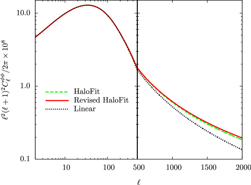
Figure 1: The angular power spectrum of the gradient mode generated by matter density fluctuations with the linear matter power spectrum (black dotted), and with fitting formula of the non-linear matter power spectrum given in Ref. Smith:2002dz (green dashed) or Takahashi:2012em (red solid).

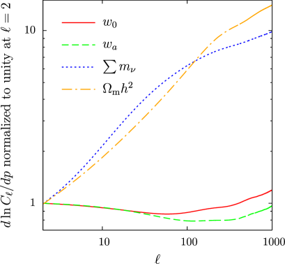
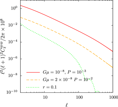
Figure 2: Left : Logarithmic derivatives of the gradient-mode power spectrum ${\rm d}\ln C_{\ell}^{\phi\phi}/{\rm d}p$ with respect to the dark-energy equation-of-state parameters, $w_{0}$ (red solid), $w_{a}$ (green dashed), total mass of neutrinos, $\sum m_{\nu}$ (blue dotted) and $\Omega_{\rm m}h^{2}$ (orange long-dashed). The derivatives are normalized with the value at $\ell=2$. Note that the sign of the derivative with respect to $\Omega_{\rm m}h^{2}$ is positive, while the others have negative sign. Right : The angular power spectrum of the curl mode generated by the primordial gravitational waves with the tensor-to-scalar ratio $r=0.1$ (green dotted) and a specific model of the cosmic-string network (red solid/orange dashed).

Fig. 1 shows the angular power spectrum of the gradient mode generated by the matter density fluctuations. Three lines show the case with different fitting formulas of the matter power spectrum, i.e., the halofit model Smith:2002dz and its revised formula Takahashi:2012em in calculating angular power spectrum. For comparison, we also show the case with the linear power spectrum. Note that the lensing power spectrum is computed with CAMB Lewis:1999bs . The linear approximation to the matter power spectrum would be accurate at the scales where the signal becomes large ($\ell\sim 10-100$). The non-linear growth of matter density perturbations enhances the amplitude with $20$ - $30\%$ at $\ell\sim 2000$ compared to linear theory. The sensitivity of $C_{\ell}^{\phi\phi}$ to the models of the non-linear evolution would be not so significant even at these scales, because the lensing power spectrum computed with the halofit model of Ref. Smith:2002dz is only a few percent smaller than the revised formula.

In the left panel of Fig. 2, to see how the angular power spectrum depends on cosmological sources, we show the logarithmic derivatives of the angular power spectrum, $C_{\ell}^{\phi\phi}$ with respect to $w_{0}$ and $w_{a}$, a parameterization of the dark-energy equation-of-state as $w=w_{0}+(1-a)w_{a}$, and the total mass of neutrinos $\sum m_{\nu}$. For comparison, we also show dependence on the matter density $\Omega_{\rm m}h^{2}$. Note that the derivatives are normalized with a value at $\ell=2$. The derivatives with respect to the neutrino mass depend on $\ell$, since the presence of the massive neutrinos suppresses the matter density fluctuations at smaller scales than their free-streaming scale after they become non-relativistic particles 1980:Bond . On the other hand, the derivatives with respect to $w_{0}$ and $w_{a}$ are almost scale-independent because the density fluctuations are affected by the properties of the dark energy through the evolution of the scale factor in the linear perturbation regime. These behaviors imply that the power spectrum of the gradient mode can distinguish the effect of the neutrino mass from that of the dark energy through the scale dependence Kaplinghat:2003bh . We note however that there exist some parameters that exhibit a similar scale-dependence of the total neutrino mass, which can be a source of parameter degeneracy (see e.g., Namikawa:2010re ). As shown in Fig. 2, the logarithmic derivative with respect to the matter density gives a similar trend to that of the neutrino mass. This is because the matter density changes not only the amplitude of matter density fluctuations but also shift the peak of the matter power spectrum which is determined by the radiation-matter equality. Within the CMB data set, the degeneracy between the total mass of neutrinos and matter density remains and other external dataset would be required to break this degeneracy.

On the other hand, in the right panel of Fig. 2, we show examples of the curl-mode angular power spectrum generated by the primordial gravitational waves with the tensor-to-scalar ratio $r=0.1$, and a specific model of cosmic string networks Yamauchi:2011cu parametrized by the tension $G\mu$ and reconnection probability $P$. The angular power spectrum decreases at smaller scales since the perturbations are suppressed at sub-horizon scale. That is, a measurement of the curl-mode power spectrum on large scale is important to probe the primordial-gravitational waves and cosmic-string networks.

3 Lensing effect on CMB anisotropies

Lensing effect on CMB anisotropies modifies the statistical properties of the observed CMB anisotropies. The non-Gaussian behavior in the lensed anisotropies is particularly important for measuring the angular power spectrum of the gradient and curl modes as discussed in the next section. In this section, we briefly summarize the weak lensing effect on the angular power spectrum of CMB temperature and polarization, and non-Gaussian statistics such as the bispectrum and trispectrum, in the presence of both the gradient and curl modes (see also Ref. Smith:2011we for a review on the non-Gaussian statistics by lensing).

3.1 Lensed CMB angular power spectrum

The lensed temperature anisotropies $\widetilde{\Theta}(\hat{\bm{n}})$ are expressed as a remapping of unlensed temperature anisotropies $\Theta(\hat{\bm{n}})$ by a deflection angle (e.g., Blanchard:1987AA ):

$$\widetilde{\Theta}(\hat{\bm{n}})=\Theta(\hat{\bm{n}}+\bm{d}(\hat{\bm{n}}))\,.$$ (33)

The lensing effect on the CMB polarization is also described as a remapping of the Stokes parameters $Q\pm{\rm i}\hskip 0.50003ptU$ by the deflection angle.

To analyze the asymptotic property of the lensed angular power spectrum, it is convenient to express the angular power spectrum in the flat-sky approximation. If we consider a small patch on a unit sphere and ignore the sky curvature, the CMB anisotropies are approximately given on a two-dimensional plane. In this limit, the lensed temperature anisotropies are expanded in terms of the plane wave:

$$\widetilde{\Theta}(\hat{\bm{n}}) ={\int\!\!\frac{\,{\rm d}^{2}\bm{\ell}\,}{(2\pi)^{2}}\,}\widetilde{\Theta}_{\bm{\ell}}\hskip 1.00006pt{\rm e}^{{\rm i}\hskip 0.35002pt\bm{\ell}\cdot\hat{\bm{n}}}\,.$$ (34)

On the other hand, since the lensed polarization anisotropies $\widetilde{Q}\pm{\rm i}\hskip 0.50003pt\widetilde{U}$ are the spin $\pm 2$ quantity, we define the rotationally invariant quantities, $\widetilde{E}_{\bm{\ell}}$ and $\widetilde{B}_{\bm{\ell}}$, usually referred to as E and B modes:

$$[\widetilde{Q}\pm{\rm i}\hskip 0.50003pt\widetilde{U}](\hat{\bm{n}}) =-{\int\!\!\frac{\,{\rm d}^{2}\bm{\ell}\,}{(2\pi)^{2}}\,}(\widetilde{E}_{\bm{\ell}}\pm{\rm i}\hskip 0.50003pt\widetilde{B}_{\bm{\ell}})\hskip 1.00006pt{\rm e}^{\pm{\rm i}\hskip 0.35002pt2\varphi_{\bm{\ell}}}\hskip 1.00006pt{\rm e}^{{\rm i}\hskip 0.35002pt\bm{\ell}\cdot\hat{\bm{n}}}\,.$$ (35)

Here $\varphi_{\bm{\ell}}$ is the azimuthal angle measured from the $x$-axis of the two dimensional plane. We can also expand the unlensed CMB anisotropies and define $\Theta_{\bm{\ell}}$, $E_{\bm{\ell}}$ and $B_{\bm{\ell}}$ in the same way. The lensed (unlensed) angular power spectrum $\widetilde{C}_{\ell}$ is then defined with the Fourier multipoles as

$$\langle\widetilde{X}_{\bm{\ell}}\widetilde{Y}_{\bm{\ell}^{\prime}}\rangle=(2\pi)^{2}\delta(\bm{\ell}-\bm{\ell}^{\prime})\widetilde{C}_{\ell}^{XY}\qquad(X,Y=\Theta,E,B)\,.$$ (36)

A method to obtain the angular power spectrum is to expand the lensed anisotropies in terms of the deflection angle up to second order of the deflection angle Hu:2000ee :

$${}_{s}\widetilde{\Xi}(\hat{\bm{n}})={}_{s}\Xi(\hat{\bm{n}})+d^{a}{}_{s}\Xi_{:a}(\hat{\bm{n}})+\frac{d^{a}d^{b}}{2}{}_{s}\Xi_{:ab}(\hat{\bm{n}})\,,$$ (37)

where $s=0$ or $\pm 2$ and we define ${}_{0}\Xi=\Theta$ and ${}_{\pm 2}\Xi=Q\pm{\rm i}\hskip 0.50003ptU$. The lensed CMB anisotropies in Fourier space become Hu:2000ee ; Cooray:2005hm

$${}_{s}\widetilde{\Xi}_{\bm{\ell}} ={}_{s}\Xi_{\bm{\ell}}-\sum_{x=\phi,\varpi}{\int\!\!\frac{\,{\rm d}^{2}\bm{L}\,}{(2\pi)^{2}}\,}[(\bm{\ell}-\bm{L})\odot_{x}\bm{L}]x_{\bm{\ell}-\bm{L}}{}_{s}\Xi_{\bm{L}}\hskip 1.00006pt{\rm e}^{{\rm i}\hskip 0.35002pts\varphi_{\bm{L},\bm{\ell}}}$$

$$+\frac{1}{2}\sum_{x,y=\phi,\varpi}{\int\!\!\frac{\,{\rm d}^{2}\bm{L}\,}{(2\pi)^{2}}\,}{\int\!\!\frac{\,{\rm d}^{2}\bm{L}^{\prime}\,}{(2\pi)^{2}}\,}[\bm{L}^{\prime}\odot_{x}\bm{L}][(\bm{\ell}-\bm{L}-\bm{L}^{\prime})\odot_{y}\bm{L}^{\prime}]x_{\bm{L}^{\prime}}y_{\bm{\ell}-\bm{L}-\bm{L}^{\prime}}{}_{s}\Xi_{\bm{L}}\hskip 1.00006pt{\rm e}^{{\rm i}\hskip 0.35002pts\varphi_{\bm{L},\bm{\ell}}}\,,$$ (38)

where $\varphi_{\bm{L},\bm{\ell}}=\varphi_{\bm{L}}-\varphi_{\bm{\ell}}$ and, for arbitrary two-dimensional vectors, $\bm{a}$ and $\bm{b}$, we define the products, $\odot_{\phi}$ and $\odot_{\varpi}$, as

$$\bm{a}\odot_{\phi}\bm{b}\equiv a_{\theta}b_{\theta}+a_{\varphi}b_{\varphi}\,,\qquad\bm{a}\odot_{\varpi}\bm{b}\equiv a_{\varphi}b_{\theta}-a_{\theta}b_{\varphi}\,.$$ (39)

Using Eq. (38) and denoting the unlensed CMB angular power spectrum as $C_{\ell}$, the lensed angular power spectrum for temperature and polarization in the flat-sky approximation becomes Hu:2000ee ; Cooray:2005hm

$$\widetilde{C}^{\Theta\Theta}_{\ell} =b_{\ell}C^{\Theta\Theta}_{\ell}+\sum_{x=\phi,\varpi}{\int\!\!\frac{\,{\rm d}^{2}\bm{L}\,}{(2\pi)^{2}}\,}[\bm{L}\odot_{x}(\bm{\ell}-\bm{L})]^{2}C_{|\bm{\ell}-\bm{L}|}^{xx}C^{\Theta\Theta}_{L}\,,$$ (40)

$$\widetilde{C}^{\Theta E}_{\ell} =b_{\ell}C^{\Theta E}_{\ell}+\sum_{x=\phi,\varpi}{\int\!\!\frac{\,{\rm d}^{2}\bm{L}\,}{(2\pi)^{2}}\,}[\bm{L}\odot_{x}(\bm{\ell}-\bm{L})]^{2}C_{|\bm{\ell}-\bm{L}|}^{xx}C^{\Theta E}_{L}\cos 2\varphi_{\bm{L},\bm{\ell}}\,,$$ (41)

$$\widetilde{C}^{EE}_{\ell} =b_{\ell}C^{EE}_{\ell}+\sum_{x=\phi,\varpi}{\int\!\!\frac{\,{\rm d}^{2}\bm{L}\,}{(2\pi)^{2}}\,}[\bm{L}\odot_{x}(\bm{\ell}-\bm{L})]^{2}C_{|\bm{\ell}-\bm{L}|}^{xx}$$

$$\qquad\qquad\qquad\qquad\times\frac{1}{2}[(C^{EE}_{L}+C^{BB}_{L})+(C^{EE}_{L}-C^{BB}_{L})\cos 4\varphi_{\bm{L},\bm{\ell}}]\,,$$ (42)

$$\widetilde{C}^{BB}_{\ell} =b_{\ell}C^{BB}_{\ell}+\sum_{x=\phi,\varpi}{\int\!\!\frac{\,{\rm d}^{2}\bm{L}\,}{(2\pi)^{2}}\,}[\bm{L}\odot_{x}(\bm{\ell}-\bm{L})]^{2}C_{|\bm{\ell}-\bm{L}|}^{xx}$$

$$\qquad\qquad\qquad\qquad\times\frac{1}{2}[(C^{EE}_{L}+C^{BB}_{L})-(C^{EE}_{L}-C^{BB}_{L})\cos 4\varphi_{\bm{L},\bm{\ell}}]\,,$$ (43)

where we assume that correlation between the gradient and curl modes vanishes, and define

$$b_{\ell}=1-\ell^{2}\sum_{x=\phi,\varpi}{\int\!\!\frac{\,{\rm d}\ln L\,}{4\pi}\,}L^{4}C_{L}^{xx}=1-\frac{\ell^{2}}{2}\langle|\bm{d}|^{2}\rangle\,.$$ (44)

The lensing effect on the polarization has an interesting feature Zaldarriaga:1998ar ; even in the absence of the primary B-mode polarization, $C_{\ell}^{BB}=0$, spatial pattern of the lensed polarization anisotropies could have odd-parity mode. This is because a curl-free pattern is modified at each position and the resultant pattern is no longer a pure E-mode pattern. Note that a few arcminute deflection, $\langle|\bm{d}|^{2}\rangle\sim\mathcal{O}(10^{-7})$, Lewis:2006fu leads to $\ell^{2}\langle|\bm{d}|^{2}\rangle/2\sim\mathcal{O}(1)$ if $\ell\sim 2500$. At these scales, the above expression is no longer valid because Eqs. (40)-(43) ignore the higher order terms $\mathcal{O}(C_{\ell}^{xx})$, and a more accurate approach of Refs. Seljak:1995ve ; Zaldarriaga:1998ar is required in which the angular power spectrum is computed using the correlation function, and the higher-order terms are included non-perturbatively with an exponential function Challinor:2005jy .

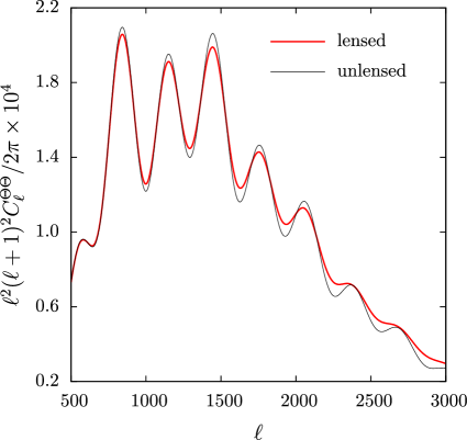
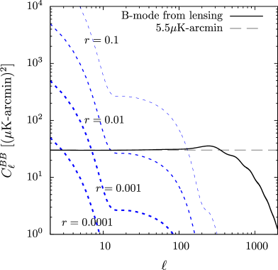
Figure 3: Summary of important signatures in the angular power spectra of the lensed anisotropies compared to those of the unlensed anisotropies. Note that contributions from the curl mode $C_{\ell}^{\varpi\varpi}$ is ignored. Left : Comparison of the angular power spectra between the lensed (red) and unlensed (black) temperature anisotropies. For illustrative purpose, we multiply $\ell^{2}(\ell+1)^{2}\times 10^{4}/2\pi$ to the angular power spectrum. Right : The angular power spectrum of the $B$-mode polarization from the primordial gravitational waves (blue dotted), compared with that from the lensing (black solid). For the primordial gravitational waves, the tensor-to-scalar ratio $r$ is varied from $0.1$ to $0.0001$. We also plot the white noise spectrum of $5.5\,\mu$K-arcmin (black dashed).

In Fig. 3, we plot the lensed angular power spectrum of the temperature (left) and B-mode polarization (right), where the angular power spectrum is computed with CAMB Lewis:1999bs . The acoustic peaks in the temperature power spectrum are smeared by the lensing effect, and this can be understood as follows. The acoustic peaks are determined by typical sizes of hot and cold temperature spots in the sky. Lensing changes the size distribution of these spots (some get bigger and some get smaller), smearing the acoustic peaks. At small scales, the temperature power spectrum is dominated by lensing due to the transfer of large-scale power to small scales, where the primary temperature fluctuations are damped. The lensing also affects the E-mode power spectrum in the similar way of the temperature case.

The B-mode power spectrum generated by the lensing effect is, on the other hand, a scale-independent spectrum on large scales ($\ell\,\raise 2.9pt\hbox{$\scriptstyle<$}\lower 0.5pt\hbox{$\scriptscriptstyle\sim$}\;100$) which roughly corresponds to $5$ - $6\mu$K-arcmin white noise. This would be considered as follows. The gradient of the primary E-mode has significant correlation on small scales, but does not correlate very much on scales larger than a few degree (or $\ell\sim 100$ Smith:2010gu ). The lensing only remaps these small scale fluctuations by typically a few arc-minute, and the resultant B-mode beyond degree scales is roughly an uncorrelated random field. This leads to the white noise spectrum on large scales.

As shown in Fig. 3, the primary B-mode power spectrum generated by the primordial gravitational waves is smaller than the lensing B-mode at recombination bump ($\ell\sim 10$-$100$) if the tensor-to-scalar ratio is $r\,\raise 2.9pt\hbox{$\scriptstyle<$}\lower 0.5pt\hbox{$\scriptscriptstyle\sim$}\;0.01$, and at reionization bump ($\ell<10$) if $r\,\raise 2.9pt\hbox{$\scriptstyle<$}\lower 0.5pt\hbox{$\scriptscriptstyle\sim$}\;0.0001$ Knox:2002pe . Therefore, if $r$ is small, detection of the primary B-mode requires subtraction of the lensing B-mode, so called delensing (see e.g., Seljak:2003pn ; Teng:2011xc ; Smith:2010gu ).

3.2 Non-Gaussian signatures of lensed CMB anisotropies

3.2.1 Bispectrum

Assuming that the primary temperature anisotropies are a random Gaussian field, the three-point correlation, $\langle\Theta_{\bm{\ell}_{1}}\Theta_{\bm{\ell}_{2}}\Theta_{\bm{\ell}_{3}}\rangle$, vanishes. As described in Eq. (38), the lensing, however, induces mode-couplings in the CMB anisotropies. The ISW-lensing correlation then generates the three-point correlation of lensed CMB anisotropies as Goldberg:1999xm

$$\langle\widetilde{\Theta}_{\bm{\ell}_{1}}\widetilde{\Theta}_{\bm{\ell}_{2}}\widetilde{\Theta}_{\bm{\ell}_{3}}\rangle=(2\pi)^{2}\delta(\bm{\ell}_{1}+\bm{\ell}_{2}+\bm{\ell}_{3})[C_{\ell_{1}}^{\Theta\phi}C^{\Theta\Theta}_{\ell_{2}}\bm{\ell}_{1}\odot_{\phi}\bm{\ell}_{2}+({\rm perms})]+\mathcal{O}(|d^{a}|^{2})\,.$$ (45)

The ISW-lensing correlation generated by density perturbations on large scale, $C_{\ell}^{\Theta\phi}$, can be used to probe the late time evolution of the large-scale structure Seljak:1998nu ; Goldberg:1999xm ; Zaldarriaga:2000ud . The cosmic strings at late time of the universe also produce the temperature bispectrum through $C_{\ell}^{\Theta\phi}$ Yamauchi:2013pna , but contributions from the curl mode vanish since the cross correlation of temperature and the curl mode is an odd-parity quantity. The curl mode generated by the cosmic strings would be, however, a source of the polarization bispectrum through, e.g., $C_{\ell}^{B\varpi}$. Note that the lensing bispectrum is a confusing source in estimating the primordial non-Gaussian signatures, especially for the squeezed type (e.g., $\ell_{1}\sim\ell_{2}\gg\ell_{3}$), and the bias for the local type becomes $f_{\rm NL}\sim\mathcal{O}(1)$ with ongoing and upcoming experiments Serra:2008wc ; Cooray:2008xz ; Hanson:2009kg . The polarization bispectrum generated by lensing is also discussed in Ref. Lewis:2011fk .

3.2.2 Trispectrum

The trispectrum of lensed CMB anisotropies has been explored Bernardeau:1996aa ; Zaldarriaga:2000ud ; Hu:2001fa and can be used to estimate the power spectrum of the gradient and curl modes as discussed in the next section.

The four-point correlation of CMB anisotropies is in general decomposed into two terms as

$$\langle\widetilde{\Theta}_{\bm{\ell}_{1}}\widetilde{\Theta}_{\bm{\ell}_{2}}\widetilde{\Theta}_{\bm{\ell}_{3}}\widetilde{\Theta}_{\bm{\ell}_{4}}\rangle=\langle\widetilde{\Theta}_{\bm{\ell}_{1}}\widetilde{\Theta}_{\bm{\ell}_{2}}\widetilde{\Theta}_{\bm{\ell}_{3}}\widetilde{\Theta}_{\bm{\ell}_{4}}\rangle_{\rm d}+\langle\widetilde{\Theta}_{\bm{\ell}_{1}}\widetilde{\Theta}_{\bm{\ell}_{2}}\widetilde{\Theta}_{\bm{\ell}_{3}}\widetilde{\Theta}_{\bm{\ell}_{4}}\rangle_{\rm c}\,,$$ (46)

where the first term is the disconnected part expressed in terms of two point correlations as

$$\langle\widetilde{\Theta}_{\bm{\ell}_{1}}\widetilde{\Theta}_{\bm{\ell}_{2}}\widetilde{\Theta}_{\bm{\ell}_{3}}\widetilde{\Theta}_{\bm{\ell}_{4}}\rangle_{\rm d}=\langle\widetilde{\Theta}_{\bm{\ell}_{1}}\widetilde{\Theta}_{\bm{\ell}_{2}}\rangle\langle\widetilde{\Theta}_{\bm{\ell}_{3}}\widetilde{\Theta}_{\bm{\ell}_{4}}\rangle+(\bm{\ell}_{2}\leftrightarrow\bm{\ell}_{3})+(\bm{\ell}_{2}\leftrightarrow\bm{\ell}_{4})\,,$$ (47)

while the second term denotes the connected part which is not expressed in terms of the two point-correlation of lensed anisotropies alone and reflects the non-Gaussian behavior of the fluctuations. The four-point correlation of the lensed temperature anisotropies has a contribution from the connected part as Kesden:2003cc

$$\langle\widetilde{\Theta}_{\bm{\ell}_{1}}\widetilde{\Theta}_{\bm{\ell}_{2}}\widetilde{\Theta}_{\bm{\ell}_{3}}\widetilde{\Theta}_{\bm{\ell}_{4}}\rangle_{\mathrm{c}} \simeq(2\pi)^{2}\delta(\bm{\ell}_{1}+\bm{\ell}_{2}+\bm{\ell}_{3}+\bm{\ell}_{4})$$

$$\qquad\times\sum_{x=\phi,\varpi}\left\{C_{|\bm{\ell}_{1}+\bm{\ell}_{2}|}^{xx}f^{x}_{\bm{\ell}_{1}+\bm{\ell}_{2},\bm{\ell}_{1}}f^{x}_{\bm{\ell}_{3}+\bm{\ell}_{4},\bm{\ell}_{3}}+(\bm{\ell}_{2}\leftrightarrow\bm{\ell}_{3})+(\bm{\ell}_{2}\leftrightarrow\bm{\ell}_{4})\right\}\,,$$ (48)

where we define a weight function as

$$f^{x}_{\bm{L},\bm{L}^{\prime}}=(\bm{L}\odot_{x}\bm{L}^{\prime})C^{\Theta\Theta}_{L^{\prime}}+(\bm{L}^{\prime}\leftrightarrow\bm{L}-\bm{L}^{\prime})\,.$$ (49)

In deriving Eq. (48), the lensed temperature anisotropies are expanded only up to first order of the gradient and curl modes. The trispectrum of polarization generated by the lensing effect is also obtained analogously and the expression is given in Ref. Okamoto:2002ik .

3.2.3 Other statistics

There are also several papers discussing how the non-Gaussian signatures of the lensing effect change the statistical properties of a random Gaussian field, such as topological statistics Schmalzing:2000 ; Takada:2001b , and the two-point correlation of hot spots Takada:2000 ; Takada:2001a . Non-zero lensing trispectrum also modifies the covariance of the lensed CMB angular power spectrum Smith:2005ue ; Smith:2006nk ; Li:2006pu ; BenoitLevy:2012va .

4 Lensing Reconstruction

Estimators for the lensing deflection fields in quadratic form of observed CMB anisotropies have been derived by several authors. Refs. Zaldarriaga:1998te ; Seljak:1998aq developed a method for extracting lensing fields from temperature anisotropies with real space quantities. The method was subsequently extended to the case with polarization Guzik:2000ju . The quadratic estimator mostly used in the recent analysis was developed in Fourier space by Refs. Hu:2001 ; Hu:2001kj and Okamoto:2003zw in flat and full sky, respectively, and was also extended to include the curl mode by Ref. Cooray:2005hm in flat sky and by Ref. Namikawa:2011cs in full sky. On the other hand, the estimator is also derived in the context of the maximum likelihood Hirata:2002jy ; Hirata:2003ka . These estimators all utilize the fact that a fixed gradient/curl mode introduces statistical anisotropy into the observed CMB, in the form of a correlation between the CMB anisotropies and its gradient. With a large number of observed CMB modes, this correlation may be used to form estimates of the gradient and curl modes. The lensing power spectrum, which is required for cosmological analysis is then estimated from the gradient/curl mode estimators.

In this section, to see how to estimate the lensing power spectrum, $C_{\ell}^{\phi\phi}$ and $C_{\ell}^{\varpi\varpi}$, we first review the method for estimating the gradient and curl modes, usually referred to as lensing reconstruction, and their use of measuring the angular power spectrum (see also Hanson:2009kr for a detailed review on the lensing reconstruction). Since the lensing fields would be measured more precisely in the near future, we also discuss the method for estimating lensing fields and their power spectrum with better accuracy.

4.1 Estimating CMB lensing potentials

4.1.1 Quadratic estimator for gradient and curl modes

For simplicity, let us first consider an estimator with a CMB temperature map alone in the absence of curl modes. In the following, observed temperature anisotropies and their angular power spectrum are denoted as $\widehat{\Theta}_{\bm{\ell}}$ and $\widehat{C}^{\Theta\Theta}_{\ell}$, respectively. We assume that the observed anisotropies are given by $\widehat{\Theta}_{\bm{\ell}}=\widetilde{\Theta}_{\bm{\ell}}+n_{\bm{\ell}}$ where $n_{\bm{\ell}}$ is the isotropic noise.

The observed direction of the lensed CMB at each position is shifted from the original direction according to the deflection angle, and the distance between two positions are modified at each position in a different way. For a fixed realization of the deflection angle, the correlation function of the primary CMB anisotropies depends not only on the distance between two positions but also on the position in the sky. In Fourier space, the lensing-induced anisotropy leads to the correlations between two different Fourier modes of the observed CMB anisotropies.

$$\langle\widehat{\Theta}_{\bm{L}}\widehat{\Theta}_{\bm{\ell}-\bm{L}}\rangle_{\mathrm{CMB,n}}=\phi_{\bm{\ell}}f^{\phi}_{\bm{\ell},\bm{L}}\,,\quad(\bm{\ell}\not=\bm{0})$$ (50)

where $f^{\phi}_{\bm{\ell},\bm{L}}$ is given in Eq. (49), and we denote the ensemble average over primary CMB anisotropies and noise by $\langle\cdots\rangle_{\mathrm{CMB,n}}$, to distinguish it from the usual meaning of the ensemble average, $\langle\cdots\rangle$.

Based on Eq. (50), the quantity, $\widehat{\phi}_{\bm{\ell},\bm{L}}$, defined as

$$f^{\phi}_{\bm{\ell},\bm{L}}\widehat{\phi}_{\bm{\ell},\bm{L}}=\widehat{\Theta}_{\bm{L}}\widehat{\Theta}_{\bm{\ell}-\bm{L}}\,.$$ (51)

is an estimator which satisfies the unbiased condition : $\langle\widehat{\phi}_{\bm{\ell},\bm{L}}\rangle_{\mathrm{CMB,n}}=\phi_{\bm{\ell}}$ where $\bm{L}$ is chosen so that $f_{\bm{\ell},\bm{L}}^{\phi}\not=0$. . A more optimal and unbiased estimator can be obtained as a sum of $\widehat{\phi}_{\bm{\ell},\bm{L}}$ in terms of $\bm{L}$, and the resultant estimator is Hu:2001

$$\widehat{\phi}_{\bm{\ell}}=A^{\phi}_{\ell}{\int\!\!\frac{\,{\rm d}^{2}\bm{L}\,}{(2\pi)^{2}}\,}g^{\phi}_{\bm{\ell},\bm{L}}\widehat{\Theta}_{\bm{L}}\widehat{\Theta}_{\bm{\ell}-\bm{L}}\,.$$ (52)

Here the normalization, $A^{\phi}_{\ell}$, and the weight function, $g^{\phi}_{\bm{\ell},\bm{L}}$ are given by

$$A^{\phi}_{\ell}=\frac{1}{[g^{\phi},f^{\phi}]_{\bm{\ell}}}\,;\quad g^{\phi}_{\bm{\ell},\bm{L}}=\frac{f^{\phi}_{\bm{\ell},\bm{L}}}{2\widehat{C}^{\Theta\Theta}_{L}\widehat{C}^{\Theta\Theta}_{|\bm{\ell}-\bm{L}|}}\,,$$ (53)

where, for convenience, the inner product is defined as

$$[g^{x},f^{y}]_{\bm{\ell}}\equiv{\int\!\!\frac{\,{\rm d}^{2}\bm{L}\,}{(2\pi)^{2}}\,}g^{x}_{\bm{\ell},\bm{L}}f^{y}_{\bm{\ell},\bm{L}}\,.$$ (54)

In the presence of the curl mode, Eq. (50) includes the additional term induced by the curl mode:

$$\langle\widehat{\Theta}_{\bm{L}}\widehat{\Theta}_{\bm{\ell}-\bm{L}}\rangle_{\mathrm{CMB,n}}=\phi_{\bm{\ell}}f^{\phi}_{\bm{\ell},\bm{L}}+\varpi_{\bm{\ell}}f^{\varpi}_{\bm{\ell},\bm{L}}\,.$$ (55)

Even in this case, the estimator for the gradient mode is the same as in Eq. (52), at least, if we consider the first order of the gradient and curl modes. This is because the property of the parity symmetry is different for the gradient and curl modes, and the inner product $[f^{\phi},f^{\varpi}]_{\bm{\ell}}$, which leads to a bias in the gradient-mode estimator, vanishes Namikawa:2011cs . The quadratic estimators with the polarization anisotropies are also constructed in the same way as in the temperature case. The optimal quadratic estimator is finally obtained by combining all quadratic combinations of temperature and polarization fluctuations with the appropriate weight functions Hu:2001kj .

4.1.2 Practical cases

In practical situations, any non-lensing anisotropies arising from the masking vanEngelen:2012va ; Namikawa:2012pe ; BenoitLevy:2013bc , inhomogeneous map noise Hanson:2009dr and the beam asymmetry coupled with the scan strategy Hanson:2010gu will also generate the off-diagonal elements in the covariance matrix similar to Eq. (50), and the quadratic estimator is biased, i.e., $\langle\widehat{x}_{\bm{\ell}}\rangle_{\mathrm{CMB,n}}\not=0$. In the case of polarization, there are also several possible sources generating mode-couplings such as the temperature to polarization leakage, rotation of polarization basis and so on Shimon:2007au .

To see this, let us consider a modulation on temperature anisotropies given by

$$\widehat{\Theta}(\hat{\bm{n}})=(1+\epsilon(\hat{\bm{n}}))(\widetilde{\Theta}(\hat{\bm{n}})+n(\hat{\bm{n}}))\,,$$ (56)

where $\epsilon(\hat{\bm{n}})$ may be regarded as the window function, inhomogeneity of the optical depth Gluscevic:2012qv ; O'Bryan:2013bea , Doppler boosting Aghanim:2013suk ; Hanson:2009gu , and so on. The off-diagonal covariance of temperature anisotropies in the absence of the curl mode is given by at the first order

$$\langle\widehat{\Theta}_{\bm{L}}\widehat{\Theta}_{\bm{\ell}-\bm{L}}\rangle_{\mathrm{CMB,n}}=f^{\phi}_{\bm{\ell},\bm{L}}\phi_{\bm{\ell}}+f^{\epsilon}_{\bm{\ell},\bm{L}}\epsilon_{\bm{\ell}}\,.$$ (57)

where $f^{\epsilon}_{\bm{\ell},\bm{L}}=\widehat{C}^{\Theta\Theta}_{L}+\widehat{C}^{\Theta\Theta}_{|\bm{\ell}-\bm{L}|}$. Substituting the above equation to Eq. (52), we obtain

$$\langle\widehat{\phi}_{\bm{\ell}}\rangle_{\mathrm{CMB,n}}=\phi_{\bm{\ell}}+R_{\ell}^{\phi,\epsilon}\epsilon_{\bm{\ell}}\,,$$ (58)

where the response function, $R_{\ell}^{\phi,\epsilon}$, or in general, $R_{\ell}^{a,b}$, is defined as

$$R_{\ell}^{a,b}=\frac{A^{a,a}_{\ell}}{A^{a,b}_{\ell}}\,;\qquad A_{\ell}^{a,b}=\frac{1}{[g^{a},f^{b}]_{\ell}}\,.$$ (59)

The second term of Eq. (58) is called the mean-field bias, and must be corrected.

One of the methods to correct the mean-field bias is to construct an estimator for $\epsilon_{\bm{\ell}}$. Similar to the lensing estimator, the estimator for $\epsilon_{\bm{\ell}}$ is constructed using the weight function $f_{\bm{\ell},\bm{L}}^{\epsilon}$ instead of $f_{\bm{\ell},\bm{L}}^{\phi}$. The estimator of $\epsilon_{\bm{\ell}}$ is, however, biased by the presence of lensing as

$$\langle\widehat{\epsilon}_{\bm{\ell}}\rangle_{\mathrm{CMB,n}}=\epsilon_{\bm{\ell}}+R_{\ell}^{\epsilon,\phi}\phi_{\bm{\ell}}\,,$$ (60)

where $R_{\ell}^{\epsilon,\phi}$ is defined in Eq. (59). Combining Eqs. (58) and (60) to eliminate the term proportional to $\epsilon_{\bm{\ell}}$, we find an unbiased estimator for the gradient mode:

$$\widehat{\phi}^{\prime}_{\bm{\ell}}=\frac{\widehat{\phi}_{\bm{\ell}}-R_{\ell}^{\phi,\epsilon}\widehat{\epsilon}_{\bm{\ell}}}{1-R_{\ell}^{\phi,\epsilon}R_{\ell}^{\epsilon,\phi}}\,.$$ (61)

Note that the above estimator is derived as the optimal estimator in the case when $\phi_{\bm{\ell}}$ and $\epsilon_{\bm{\ell}}$ are simultaneously estimated.

Even if we know the property of $\epsilon_{\bm{\ell}}$ (e.g., the window function), the estimator defined in Eq. (61) is useful as a cross check of systematics propagated from imperfect understanding of underlying CMB anisotropies Namikawa:2012pe . The similar method can be also applied to reduce the inmohogeneous noise, unresolved point sources, polarization angle systematics Namikawa:2012pe ; Ade:2013tyw , as well as for polarization-based reconstruction to reduce bias from the temperature-to-polarization leakage, rotation of polarization basis, and so on Namikawa:2013 .

4.1.3 Maximum Likelihood Estimator

Here we comment on the maximum-likelihood estimator of Refs. Hirata:2002jy ; Hirata:2003ka (see also Ref. Hanson:2009kr for a thorough review). Given a set of observed CMB anisotropies, we can formally derive the estimator for the lensing fields based on maximizing the likelihood. Although the numerical calculation of the maximum-likelihood estimator is difficult compared to the quadratic estimator, it is possible to improve the precision of the estimated gradient and curl modes. For the gradient mode, the expression of the maximum-likelihood estimator is nearly identical to that of the quadratic estimator if we only use the temperature anisotropies for the lensing reconstruction Hirata:2002jy . On the other hand, as shown in Ref. Hirata:2003ka , the maximum-likelihood estimator with the B-mode polarization significantly improves the sensitivity to the lensing signals, compared to the quadratic estimator. This is because the sensitivity of the maximum-likelihood estimator is limited by the intrinsic scatter of the primary CMB anisotropies while the sensitivity of the quadratic estimator is limited by the lensed CMB anisotropies. These situations would be also similar for the curl mode. The quadratic estimator is still useful for experiments with the polarization sensitivity of $\raise 2.9pt\hbox{$\scriptstyle>$}\lower 0.5pt\hbox{$\scriptscriptstyle\sim$}\;5\mu$K-arcmin which corresponds to the amplitude of the B-mode polarization at $\ell\,\raise 2.9pt\hbox{$\scriptstyle<$}\lower 0.5pt\hbox{$\scriptscriptstyle\sim$}\;1000$.

4.2 Estimating CMB lensing power spectrum

The angular power spectrum of the gradient and curl modes may be studied through the angular power spectrum of the estimators discussed in the previous section. The angular power spectrum of the quadratic estimators, however, includes additional contributions from, e.g., the four-point correlation of the lensed CMB anisotropies, and methods to accurately estimate these bias terms are required.

To see this, from Eq. (52), we consider the angular power spectrum of the quadratic estimator with temperature which is given by

$$\langle|\widehat{x}_{\bm{\ell}}|^{2}\rangle=(A_{\ell}^{x})^{2}{\int\!\!\frac{\,{\rm d}^{2}\bm{L}\,}{(2\pi)^{2}}\,}{\int\!\!\frac{\,{\rm d}^{2}\bm{L}^{\prime}\,}{(2\pi)^{2}}\,}\frac{f^{x}_{\bm{\ell},\bm{L}}}{2\widehat{C}^{\Theta\Theta}_{L}\widehat{C}^{\Theta\Theta}_{|\bm{\ell}-\bm{L}|}}\frac{f^{x}_{\bm{\ell},\bm{L}^{\prime}}}{2\widehat{C}^{\Theta\Theta}_{L^{\prime}}\widehat{C}^{\Theta\Theta}_{|\bm{\ell}-\bm{L}^{\prime}|}}\langle\widehat{\Theta}_{\bm{L}}\widehat{\Theta}_{\bm{\ell}-\bm{L}}(\widehat{\Theta}_{\bm{L}^{\prime}}\widehat{\Theta}_{\bm{\ell}-\bm{L}^{\prime}})^{*}\rangle\,.$$ (62)

This quantity probes the 4-point function of the lensed CMB. Following Eq. (46), we decompose the above quantity into disconnected and connected parts :

$$\langle|\hat{x}_{\bm{\ell}}|^{2}\rangle=\langle|\hat{x}_{\bm{\ell}}|^{2}\rangle_{\mathrm{d}}+\langle|\hat{x}_{\bm{\ell}}|^{2}\rangle_{\mathrm{c}}\,.$$ (63)

The disconnected part, $\langle\cdots\rangle_{\mathrm{d}}$, which comes from Eq. (47), contains the contributions which would be expected if the observed temperature anisotropies $\widehat{\Theta}_{\bm{L}}$ were a Gaussian random variable. On the other hand, the connected part, $\langle\cdots\rangle_{\mathrm{c}}$, arising from Eq. (48), has the non-Gaussian contributions which are a distinctive signature of lensing. As shown in the following, the connected part nearly corresponds to the power spectrum of the gradient/curl mode, and therefore the disconnected part, usually referred to as “Gaussian bias”, and the other bias terms must be accurately subtracted to obtain a clean measurement of the lensing signals.

Let us discuss the explicit expression of the disconnected and connected part.

• Disconnected part :
  Using Eq. (47), the explicit form of the Gaussian bias is written as

  $$\langle\widehat{\Theta}_{\bm{L}}\widehat{\Theta}_{\bm{\ell}-\bm{L}}(\widehat{\Theta}_{\bm{L}^{\prime}}\widehat{\Theta}_{\bm{\ell}-\bm{L}^{\prime}})^{*}\rangle_{\mathrm{d}}=(2\pi)^{2}[\delta_{D}(\bm{L}+\bm{L}^{\prime})+\delta_{D}(\bm{L}+\bm{L}^{\prime}-\bm{\ell})]\widehat{C}_{L}^{\Theta\Theta}\widehat{C}_{|\bm{\ell}-\bm{L}|}^{\Theta\Theta}\,.$$ (64)

  Substituting Eq.(64) into Eq.(62), and using the expression of the normalization $A_{\ell}^{x}$, the power spectrum of the estimator induced by the disconnected part becomes

  $$N_{\ell}^{x,(0)}\equiv\langle|\widehat{x}_{\bm{\ell}}|^{2}\rangle_{\mathrm{d}}=\left\{{\int\!\!\frac{\,{\rm d}^{2}\bm{L}\,}{(2\pi)^{2}}\,}\frac{(f^{x}_{\bm{\ell},\bm{L}})^{2}}{2\widehat{C}^{\Theta\Theta}_{L}\widehat{C}^{\Theta\Theta}_{|\bm{\ell}-\bm{L}|}}\right\}^{-1}=A_{\ell}^{x}\,.$$ (65)

• Connected part :
  Substituting Eq. (48) into Eq. (62), the connected part of the quadratic estimator is, on the other hand, given by Kesden:2003cc

  $$\langle|\hat{x}_{\bm{\ell}}|^{2}\rangle_{\mathrm{c}}=C_{\ell}^{xx}+N_{\ell}^{x,(1)}+\mathcal{O}[(C_{\ell}^{xx})^{2}]\,.$$ (66)

  Here $C_{\ell}^{xx}$ is the gradient-mode power spectrum which we wish to estimate, while $N_{\ell}^{x,(1)}$ is a nuisance term coming from the “secondary” lensing contractions of the trispectrum Hu:2001fa which is usually called the N1 bias.

Combining Eqs. (65) and (66) with Eq. (63), we obtain

$$\langle|\hat{x}_{\bm{\ell}}|^{2}\rangle=C_{\ell}^{xx}+N_{\ell}^{x,(0)}+N^{x,(1)}_{\ell}+\mathcal{O}[(C_{\ell}^{xx})^{2}]\,.$$ (67)

The above equation means that the lensing power spectrum $C_{\ell}^{xx}$ is measured by computing the power spectrum of the lensing estimator and subtracting the accurate estimation of bias terms such as $N_{\ell}^{x,(0)}$ and $N^{x,(1)}_{\ell}$.

The Gaussian bias is usually larger than the gradient/curl-mode power spectrum for reconstructions with noisy map. A method to improve sensitivity to $C_{\ell}^{xx}$ is to use an observed map filtered by a realization-dependent power spectrum, instead of its ensemble-averaged quantities Dvorkin:2009ah in Eq. (65). In addition, the realization-dependent estimate has an advantage to reduce the off-diagonal covariance, $\langle\widehat{C}^{\phi\phi}_{\ell}\widehat{C}^{\phi\phi}_{\ell^{\prime}}\rangle$ Hanson:2010rp . For practical situations in which the covariance of observed map has non-negligible off-diagonal components, the following estimator is useful as a realization-dependent approach Namikawa:2012pe

$$\widehat{N}_{\ell}^{x,(0)}=\left(A_{\ell}^{x}\right)^{2}\frac{1}{2}{\int\!\!\frac{\,{\rm d}^{2}\bm{L}\,}{(2\pi)^{2}}\,}{\int\!\!\frac{\,{\rm d}^{2}\bm{L}^{\prime}\,}{(2\pi)^{2}}\,}f^{x}_{\bm{\ell},\bm{L}}f^{x}_{\bm{\ell},\bm{L}^{\prime}}\left(2\overline{{\bm{\mathrm{C}}}}_{\bm{L},\bm{\ell}-\bm{L}^{\prime}}\overline{\Theta}_{\bm{\ell}-\bm{L}}\overline{\Theta}_{\bm{L}^{\prime}}^{*}-\overline{{\bm{\mathrm{C}}}}_{\bm{L},\bm{\ell}-\bm{L}^{\prime}}\overline{{\bm{\mathrm{C}}}}_{\bm{\ell}-\bm{L},\bm{L}^{\prime}}\right)\,.$$ (68)

Here $\overline{\Theta}_{\bm{\ell}}\equiv\sum_{\bm{\ell}^{\prime}}{\bm{\mathrm{C}}}^{-1}_{\bm{\ell},\bm{\ell}^{\prime}}\widehat{\Theta}_{\bm{\ell}^{\prime}}$ is the inverse-variance filtered multipoles and $\overline{{\bm{\mathrm{C}}}}_{\bm{\ell},\bm{\ell}^{\prime}}$ is the covariance of $\overline{\Theta}$. The above estimator is naturally derived based on the optimal estimator of trispectrum Regan:2010cn applied to lensing Namikawa:2012pe ; Ade:2013tyw , and is easily extended to include polarization Namikawa:2013 . Eq. (68) has an additional advantage for accurate estimation of $C_{\ell}^{xx}$; if the covariance is biased as $\overline{{\bm{\mathrm{C}}}}_{\bm{\ell},\bm{\ell}^{\prime}}\to\overline{{\bm{\mathrm{C}}}}_{\bm{\ell},\bm{\ell}^{\prime}}+\Sigma_{\bm{\ell},\bm{\ell}^{\prime}}$, contributions of $\Sigma_{\bm{\ell},\bm{\ell}^{\prime}}$ in Eq. (68) is at second order, while the usual method has the first-order contributions of $\Sigma_{\bm{\ell},\bm{\ell}^{\prime}}$. Another way to mitigate uncertainties in $N^{x,(0)}_{\ell}$ is that, since a large fraction of noise in the lensing reconstruction comes from the CMB fluctuations themselves, we can construct a Gaussian-bias free estimator by dividing the CMB multipoles into disjoint regions in Fourier space, with a cost of signal-to-noise Hu:2001fa ; Sherwin:2010ge . For polarization-based reconstructions, the Gaussian bias is more simply mitigated by combining, e.g., $EE$ and $EB$ estimator since the four-point correlation $\langle EEEB\rangle_{\mathrm{d}}$ vanishes.

Other bias terms such as the N1 bias $N^{x,(1)}_{\ell}$ should be also corrected. Even in the absence of the curl mode, $N^{\varpi,(1)}_{\ell}$ is generated by the presence of the gradient mode BenoitLevy:2013bc ; vanEngelen:2012va . Furthermore, Ref. Hanson:2010rp pointed out that the term including the second order of $C_{\ell}^{\phi\phi}$ in Eq. (67) also leads to non-negligible bias. This type of bias can be mitigated by replacing the unlensed power spectrum in the weight function with the lensed power spectrum Lewis:2011fk ; Anderes:2013jw . The diagonal approximation of the normalization $A_{\ell}$ would also lead to a bias in estimating the power spectrum in the presence of, e.g., the window function. The bias due to this diagonal approximation in the presence of the masking and survey boundary is not so significant for the temperature-based reconstruction Namikawa:2012pe , but would be significant on large scales for polarization-based reconstruction. For known sources such as the window effect, we would estimate the normalization bias by Monte Carlo simulations, but cross check with other methods would be desirable as a test of assumptions in simulations, e.g., underlying CMB anisotropies.

Since the power spectrum of the quadratic estimator probes the four-point correlation of observed anisotropies, other possible sources of the four-point correlation may lead to significant bias on $\widehat{C}^{xx}_{\ell^{\prime}}$. One of the significant trispectrum sources is the point sources Ade:2013tyw , and Ref. Osborne:2013nna constructed an estimator for mitigating the point-source trispectrum by modeling the statistical properties of the point sources, while Ref. vanEngelen:2013rla proposed a simulation-based approach. The bias on estimates of the power spectrum due to the presence of primordial non-Gaussianity would be also a source of the trispectrum but is negligible even even if $f_{\mathrm{NL}}\sim\mathcal{O}(10)$ Lesgourgues:2005 .

In estimating cosmological parameters with the gradient/curl-mode power spectrum, the angular power spectrum of observed CMB maps is usually added to break degeneracies between parameters. One concern in this case is the correlation of the angular power spectrum between lensed CMB and deflection angles. Assuming a Planck-like experiment with temperature alone, this correlation is negligible Schmittfull:2013 . The covariance of the angular power spectrum of lensing fields is investigated in Refs. Kesden:2003cc ; Hanson:2010rp , and is almost diagonal for this case.

5 Recent experimental progress and future prospect

5.1 Current status of observations

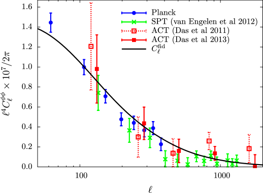
Figure 4: Measurements of the angular power spectrum of the gradient mode obtained from Planck Ade:2013tyw , SPT vanEngelen:2012va , and ACT Das:2011ak ; Das:2013zf , with the temperature-based lensing reconstruction. The solid line shows the theoretical power spectrum expected from the best-fit cosmological parameters to the Planck temperature data.

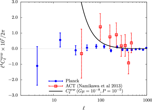
Figure 5: Same as Fig. 4 but for the curl mode obtained from Planck Ade:2013tyw and ACT temperature map Namikawa:2013wda . The solid line shows the theoretical power spectrum for a specific model of cosmic-string network with $G\mu=10^{-8}$ and $P=10^{-5}$. Note that the curl mode from SPT temperature data is also analyzed in Ref. vanEngelen:2012va .

Table 1: Current observational status of the measurement of the CMB lensing power spectrum and cross power spectrum with other data. Each column shows the gradient-mode power spectrum ($\phi\times\phi$), the cross-correlation with the galaxy/quasar catalog ($\phi\times G$), the cosmic-infrared background map ($\phi\times$CIB) or other probes such as the cosmic shear ($\phi\times\gamma$), the integrated Sachs-Wolfe effect ($\phi\times$ISW) and thermal Sunyaev-Zel’dovich effect ($\phi\times$tSZ). Note that part of the results is obtained by combining additional data e.g., WMAP. We also note that the lensing effect has been measured from the power spectrum of CMB anisotropies with several experiments (see text for details).

Temperature
	$\phi\times\phi$	$\phi\times$G	$\phi\times$CIB	$\phi\times$ other probes
ACT	$4\,\sigma$ Das:2011ak	$3.8\,\sigma$ Sherwin:2012mr	—	$3.2\,\sigma$ Hand:2013xua ($\times\gamma$)
	$4.6\,\sigma$ Das:2013zf
Planck	$26\,\sigma$ Ade:2013tyw	$7\,\sigma$ - $20\,\sigma$ Ade:2013tyw	$42\,\sigma$ Ade:2013aro a	$2.5\,\sigma$ Ade:2013dsi ($\times$ISW)
				$6.2\,\sigma$ Hill:2013dxa ($\times$tSZ)
SPT	$6.3\,\sigma$ vanEngelen:2012va	$4.2$ - $5.3\,\sigma$ Bleem:2012gm	$8.8\,\sigma$ Holder:2013hqu	—
		$\sim 7\,\sigma$ Geach:2013zwa		—
WMAP	— b	$\sim 3\,\sigma$ Smith07 ; Hirata:2008cb ; Feng:2012uf c	—	— d
Polarization
	$\phi\times\phi$	$\phi\times$G	$\phi\times$CIB	$\phi\times$ other probes
PolarBear	$\sim 2\,\sigma$ PB1:2013a e	—	$4.0\,\sigma$ PB1:2013b	—
SPTpol	$\sim 3\,\sigma$ Hanson:2013daa f	—	$7.7\,\sigma$ Hanson:2013daa	—

• Statistical significance at 545 GHz.

• Ref. Feng:2011jx showed that the significance is $\raise 2.9pt\hbox{$\scriptstyle<$}\lower 0.5pt\hbox{$\scriptscriptstyle\sim$}\;1$ - $2\,\sigma$.

• The measurement of the cross-correlation was first attempted by Ref. Hirata:2004rp , but the signals are not detected.

• Statistical significance of cross-correlation with the sum of SZ and ISW is at $\raise 2.9pt\hbox{$\scriptstyle<$}\lower 0.5pt\hbox{$\scriptscriptstyle\sim$}\;1$ - $2\,\sigma$ Calabrese:2009bu .

• The statistical significance for the rejection of the null hypothesis is at $4.6\,\sigma$.

• Ref. Hanson:2013daa constrained the lensing amplitude as a consistency test.

Observations of the lensing effect on CMB are rapidly improving (see Table 1). Combining the Arcminute Cosmology Bolometer Array Receiver (ACBAR) with the Wilkinson Microwave Anisotropy Probe (WMAP) data, Ref. Reichardt:2008ay reported a weak evidence of the lensing effect on the temperature power spectrum by constraining a parameter $q$ which characterizes the lensing effect as $C_{\ell}^{\rm lens}=C_{\ell}^{\rm no-lens}+q(C_{\ell}^{\rm lens}-C_{\ell}^{\rm no-lens})$. On the other hand, Ref. Calabrese:2009tt showed a constraint on the lensing amplitude $A$ by replacing $C_{\ell}^{\phi\phi}\to AC_{\ell}^{\phi\phi}$ in computing the lensed temperature power spectrum, and found $A=3.0^{+0.9}_{-0.9}$ while Ref. Reichardt:2008ay showed $A=1.60^{+0.55}_{-0.26}$. The lensing effect on the temperature power spectrum has been also explored by several high-resolution experiments such as the Atacama Cosmology Telescope (ACT) Das:2010ga and South Pole Telescope (SPT) Keisler:2011aw ; Story:2012wx . The recent Planck result Ade:2013zuv showed clear evidence for the lensing effect on the temperature power spectrum at $\raise 2.9pt\hbox{$\scriptstyle>$}\lower 0.5pt\hbox{$\scriptscriptstyle\sim$}\;10\,\sigma$ statistical significance . The polarization signals have been also used to show evidence for the lensing effect on the CMB anisotropies. The recent SPTpol results showed the detection of B-mode polarization signals generated from the lensing effect by cross-correlating a map of the cosmic-infrared background obtained from the Herschel Hanson:2013daa . Using the polarization data obtained from the PolarBear experiment, the B-mode maps were also used to measure the B-mode angular power spectrum Ade:2014afa .

As shown in Fig. 4, the power spectrum of the gradient mode obtained through the lensed CMB trispectrum has been also explored by several CMB experiments. The power spectrum has been measured at $\sim 4\,\sigma-6\,\sigma$ significance based on the ACT Das:2011ak ; Das:2013zf or SPT vanEngelen:2012va temperature maps. At the time of writing this paper, the most precise measurement of the power spectrum is given by the Planck with greater than $25\,\sigma$ detection Ade:2013tyw . CMB polarization maps from the SPTpol Hanson:2013daa and PolarBear PB1:2013a are also utilized to measure the gradient-mode power spectrum. As shown in Fig. 5, the curl-mode power spectrum has been measured with ACT Namikawa:2013wda , SPT vanEngelen:2012va and Planck temperature maps Ade:2013tyw , and is consistent with zero.

There are also several efforts to measure the cross correlation between the CMB lensing and other observables. Cross-correlation with matter density fluctuations is detected at $2$-$3\,\sigma$ significance with the data set of WMAP and observations of the large-scale structure such as Sloan Digital Sky Survey (SDSS) and NRAO VLA Sky Survey (NVSS) Smith07 ; Hirata:2008cb . The first detection of the cross-correlation was made earlier than the measurements of the gradient-mode power spectrum. The galaxy/quasar-CMB lensing cross-correlation has been also measured by Refs. Sherwin:2012mr ; Bleem:2012gm ; Ade:2013tyw . Cross correlations with map of the cosmic-infrared background has been also measured and utilized to estimate the bias factor of dusty sources Holder:2013hqu and the star formation rate Ade:2013aro . This correlation is more significant than the cross-correlation with the galaxy/quasar number density since the cosmic-infrared background is sensitive to the density fluctuations of dark matter mostly around $z\sim 2$, corresponding to the peak of the CMB lensing kernel Song:2002sg . Ref. Hand:2013xua reported a measurement of the cross correlation with the cosmic shear using data from the ACT and Canada-France-Hawaii Telescope (CFHT) Stripe 82 Survey (CS82). Measurements of cross-correlations with other CMB secondaries such as the integrated Sachs-Wolfe effect and thermal Sunyaev-Zel’dovich effect are reported in Refs. Ade:2013dsi and Hill:2013dxa , respectively.

The lensing signals are now one of the standard probes in cosmology, and have been already used for several cosmological issues. The inclusion of the gradient-mode power spectrum breaks degeneracies of parameters involved in the angular-diameter distance to the last scattering Hu:2001fb , e.g., the dark energy density $\Omega_{\Lambda}$ and curvature parameter $\Omega_{\mathrm{K}}$, whose degeneracies are difficult to break only with the primary CMB anisotropies alone Zaldarriaga:1997ch ; Bond:1997wr ; Efstathiou:1998xx (see also about numerical effect which breaks degeneracies Howlett:2012mh ). As shown in Refs. Sherwin:2011gv ; vanEngelen:2012va ; Ade:2013tyw , combining the lensing signals with the primary CMB anisotropies provides the evidence for dark energy with CMB data alone, and the constraints on the dark energy density without any astrophysical data is now $\Omega_{\Lambda}=0.67^{+0.027}_{-0.023}\,(1\sigma)$ Ade:2013tyw . There have been several studies which used the cross correlation to some specific issues. Using the cross correlation between the lensing and galaxy survey, constraints on the primordial non-Gaussianity parameter through a measurement of the galaxy bias are obtained as $f_{\mathrm{NL}}=12\pm 21\,(1\sigma)$ Giannantonio:2013kqa . Ref. Ferraro:2014msa used the Planck lensing map to constrain the bias of Wide-Field Infrared Survey Explorer (WISE) for the purpose of estimating the ISW effect. As discussed in Sec. 2, the curl mode of lensing signals has also fruitful information on the non-scalar perturbations. Fig. 5 shows the measured curl-mode power spectrum compared with that produced by the cosmic-string network. The measured curl-mode power spectrum is used for excluding parameter region of cosmic strings Namikawa:2013wda which is not ruled out by the current data of the temperature power spectrum Ade:2013xla ; Yamauchi:2011cu .

5.2 Future prospects

CMB polarization data on arcminute scale will soon become the best way to obtain the CMB lensing power spectrum and cross-correlations, and these precise signals play an important role in cosmology in near future (see e.g., Ref. Wu:2014hta and Refs therein). This will be achieved by ongoing ground-based experiments such as ACTPol , PolarBear , and SPTpol , and upcoming/next generation experiments, e.g., Polar , CMBPol , COrE and PRISM .

Based on the above planned experiments, let us discuss the future prospect in CMB lensing studies. For the neutrinos, assuming upcoming/next-generation experiments and combining the gradient-mode power spectrum with the primary CMB power spectrum, $1\,\sigma$ constraints on the total mass of neutrinos would be $35$-$60\,{\rm meV}$ (e.g., Kaplinghat:2003bh ; Lesgourgues:2005yv ; dP09 ; Namikawa:2010re ). On the other hand, the $1\,\sigma$ constraint on the effective number of neutrinos will be $\sim 0.1$ Lesgourgues:2005yv .

The cross-correlation studies with the CMB lensing would also become important in the future. Inclusion of the cross correlations with other observables will further improve the constraints on the total mass of the neutrinos (e.g., Abazajian:2011dt ; Abazajian:2013oma and Refs therein). For example, if we combine the Stage-II class experiments with other ongoing projects such as the Subaru Hyper Suprime-Cam , the constraints on neutrino mass would be $40\,{\rm meV}$ Namikawa:2010re . In the future, with the Stage-IV class experiments and other upcoming spectroscopic survey, the constraint on the mass of neutrinos and effective number of neutrinos would be $\sim 16\,{\rm meV}$ and $0.02$, respectively Abazajian:2013oma . This implies that the lower bound on the neutrino mass $\sum m_{\nu}\sim 60\,{\rm mV}$ obtained from neutrino oscillation experiments would be detected at $4\,\sigma$ confidence level with future experiments.

For upcoming and future experiments, the auto and cross power spectrum between CMB lensing and other observables would have sensitivity to probe the dark-energy equation-of-state parameters (e.g., Hu:2001fb ; Das:2008am ; Namikawa:2010re ), a specific model of dark energy (e.g., Das:2008am ; dP09 )/modified gravity (e.g., Calabrese:2009tt ), the primordial non-Gaussianity through measurement of galaxy bias (e.g., Takeuchi:2011ej ), and the cosmic-string network (e.g., Yamauchi:2012bc ). In addition to probe the above advanced issues, the cross correlation with other probes would help to control systematics such as multiplicative bias and intrinsic alignment in the cosmic shear analysis (e.g., Vallinotto:2011ge ; Das:2013aia ; Hall:2014nja ; Troxel:2014kza ).

In the future, as mentioned in Sec. 3, the delensing may be required to obtain the primary B-mode signals at the recombination bump ($\ell\sim 10-100$). The B-mode signal at these scales would be important for ground-based experiments in which the large-scale modes are difficult to obtain. The delensing at the recombination bump is also important for future low-resolution space missions such as LiteBIRD and PIXIE Kogut:2011xw in order to enhance the total signal-to-noise of the primary B-mode as well as the sensitivity to the tensor spectral index which allows to explore the details of inflationary physics. The joint analysis for, e.g., LiteBIRD and ground-based CMB experiments would reveal the primordial B-mode signals from the largest scale to the recombination bump, providing us with much information on the primordial gravitational waves. The above estimates and prospects are however discussed in simple and idealistic situations, and studies aiming at addressing practical issues are highly required as data become precise.

References

- (1) K. N. Abazajian et al., Astropart. Phys., 35, 177–184 (2011).
- (2) K. N. Abazajian et al., arXiv:1309.5381.
- (3) K. N. Abazajian et al., arXiv:1309.5383.
- (4) E. Anderes, Phys. Rev. D (2013).
- (5) A. Benoit-Levy et al., Astron. Astrophys., 555, 10 (2013).
- (6) A. Benoit-Levy, K. M. Smith, and W. Hu, Phys. Rev., D86, 123008 (2012).
- (7) F. Bernardeau, Astron. Astrophys., 324, 15–26 (1997).
- (8) A. Blanchard and J. Schneider, Astron. Astrophys., 184, 1–6 (oct 1987).
- (9) L. E. Bleem et al., Astrophys. J., 753, L9 (2012).
- (10) J. R. Bond, G. Efstathiou, and J. Silk, Phys. Rev. Lett., 45, 1980–1984 (1980).
- (11) J. R. Bond, G. Efstathiou, and M. Tegmark, Mon. Not. Roy. Astron. Soc., 291, L33–L41 (1997).
- (12) E. Calabrese et al., Phys. Rev. D, 80, 103516 (2009).
- (13) E. Calabrese et al., Phys. Rev. D, 81, 043529 (2010).
- (14) C. S. Carvalho and K. Moodley, Phys. Rev. D, 81, 123010 (2010).
- (15) A. Challinor and A. Lewis, Phys. Rev. D, 71, 103010 (2005).
- (16) Planck Collaboration, arXiv:1303.5079.
- (17) Planck Collaboration, arXiv:1303.5076.
- (18) Planck Collaboration, arXiv:1303.5077.
- (19) Planck Collaboration, arXiv:1303.5078.
- (20) Planck Collaboration, arXiv:1303.5085.
- (21) Planck Collaboration, arXiv:1303.5087.
- (22) PolarBear Collaboration, arXiv:1312.6645.
- (23) PolarBear Collaboration, arXiv:1312.6646.
- (24) PolarBear Collaboration, arXiv:1403.2369.
- (25) A. Cooray and W. Hu, Astrophys. J., 574, 19 (2002).
- (26) A. Cooray, M. Kamionkowski, and R. R. Caldwell, Phys. Rev. D, 71, 123527 (2005).
- (27) A. Cooray, D. Sarkar, and P. Serra, Phys. Rev. D, 77, 123006 (2008).
- (28) L. Dai, M. Kamionkowski, and D. Jeong, Phys. Rev. D, 86, 125013 (2012).
- (29) S. Das, J. Errard, and D. Spergel, arXiv:1311.2338.
- (30) S. Das et al., Astrophys. J., 729, 62 (2011).
- (31) S. Das et al., Phys. Rev. Lett., 107, 021301 (2011).
- (32) S. Das et al., arXiv:1301.1037.
- (33) S. Das and D. N. Spergel, Phys. Rev. D, 79, 043509 (2009).
- (34) R. de Putter, O. Zahn, and E. V. Linder, Phys. Rev. D, 79, 065033 (2009).
- (35) S. Dodelson, E. Rozo, and A. Stebbins, Phys. Rev. Lett., 91, 021301 (2003).
- (36) C. Dvorkin, W. Hu, and K. M. Smith, Phys. Rev. D, 79, 107302 (2009).
- (37) G. Efstathiou and J. R. Bond, Mon. Not. Roy. Astron. Soc., 304, 75–97 (1999).
- (38) C. Feng et al., Phys. Rev. D, 86, 063519 (2012).
- (39) C. Feng et al., Phys. Rev. D, 85, 043513 (2012).
- (40) S. Ferraro, B. D. Sherwin, and D. N. Spergel, arXiv:1401.1193.
- (41) T. Fukushige, J. Makino, and T. Ebisuzaki, Astrophys. J., 436, L107–L110 (dec 1994).
- (42) J.E. Geach et al., Astronomical Journal, 776, L41 (2013).
- (43) T. Giannantonio and W. J. Percival, arXiv:1312.5154.
- (44) V. Gluscevic, M. Kamionkowski, and D. Hanson, arXiv:1210.5507.
- (45) D. M. Goldberg and D. N. Spergel, Phys. Rev. D, 59, 103002 (1999).
- (46) J. Guzik, U. Seljak, and M. Zaldarriaga, Phys. Rev. D, 62, 043517 (2000).
- (47) A. Hall and A. Taylor, arXiv:1401.6018.
- (48) N. Hand et al., arXiv:1311.6200.
- (49) D. Hanson, A. Challinor, and A. Lewis, Gen. Rel. Grav., 42, 2197–2218 (2010).
- (50) D. Hanson et al., Phys. Rev. D, 80, 083004 (2009).
- (51) D. Hanson et al., Phys. Rev. D, 83, 043005 (2011).
- (52) D. Hanson et al., Phys. Rev. Lett., 111, 141301 (2013).
- (53) D. Hanson and A. Lewis, Phys. Rev. D, 80, 063004 (2009).
- (54) D. Hanson, A. Lewis, and A. Challinor, Phys. Rev. D, 81, 103003 (2010).
- (55) D. Hanson, G. Rocha, and K. Gorski, Mon. Not. Roy. Astron. Soc., 400, 2169–2173 (2009).
- (56) J. C. Hill and D. N. Spergel, arXiv:1312.4525.
- (57) C. M. Hirata et al., Phys. Rev. D, 70, 103501 (2004).
- (58) C. M. Hirata et al., Phys. Rev. D, 78, 043520 (2008).
- (59) C. M. Hirata and U. Seljak, Phys. Rev. D, 67, 043001 (2003).
- (60) C. M. Hirata and U. Seljak, Phys. Rev. D, 68, 083002 (2003).
- (61) G. P. Holder et al., Astrophys. J., 771, L16 (2013).
- (62) C. Howlett et al., JCAP, 1204, 027 (2012).
- (63) W. Hu, Phys. Rev. D, 62, 043007 (2000).
- (64) W. Hu, Phys. Rev. D, 64, 083005 (2001).
- (65) W. Hu, Astrophys. J., 557, L79–L83 (2001).
- (66) W. Hu, Phys. Rev. D, 65, 023003 (2002).
- (67) W. Hu and A. Cooray, Phys. Rev. D, 63, 023504 (2001).
- (68) W. Hu and T. Okamoto, Astrophys. J., 574, 566–574 (2002).
- (69) W. Hu and M. J. White, Phys. Rev. D, 56, 596–615 (1997).
- (70) M. Kaplinghat, L. Knox, and Y.-S. Song, Phys. Rev. Lett., 91, 241301 (2003).
- (71) R. Keisler et al., Astrophys. J., 743, 28 (2011).
- (72) M. H. Kesden, A. Cooray, and M. Kamionkowski, Phys. Rev. D, 67, 123507 (2003).
- (73) L. Knox and Y.-S. Song, Phys. Rev. Lett., 89, 011303 (2002).
- (74) H. Kodama and M. Sasaki, Progress of Theoretical Physics Supplement, 78, 1 (1984).
- (75) A. Kogut et al., JCAP, 1107, 025 (2011).
- (76) J. Lesgourgues et al., Phys. Rev. D, 71, 103514 (2005).
- (77) J. Lesgourgues et al., Phys. Rev. D, 73, 045021 (2006).
- (78) A. Lewis and A. Challinor, Phys. Rep., 429, 1–65 (2006).
- (79) A. Lewis, A. Challinor, and D. Hanson, JCAP, 1103, 018 (2011).
- (80) A. Lewis, A. Challinor, and A. Lasenby, Astrophys. J., 538, 473–476 (2000).
- (81) C. Li, T. L. Smith, and A. Cooray, Phys. Rev. D, 75, 083501 (2007).
- (82) T. Namikawa, D. Hanson, and R. Takahashi, Mon. Not. Roy. Astron. Soc., 431, 609–620 (2013).
- (83) T. Namikawa, S. Saito, and A. Taruya, JCAP, 1012, 027 (2010).
- (84) T. Namikawa and R. Takahashi, Mon. Not. Roy. Astron. Soc. (2013).
- (85) T. Namikawa, D. Yamauchi, and A. Taruya, JCAP, 1201, 007 (2012).
- (86) T. Namikawa, D. Yamauchi, and A. Taruya, Phys. Rev. D (2013).
- (87) J. O’Bryan et al., arXiv:1306.1232.
- (88) T. Okamoto and W. Hu, Phys. Rev. D, 66, 063008 (2002).
- (89) T. Okamoto and W. Hu, Phys. Rev. D, 67, 083002 (2003).
- (90) S. J. Osborne, D. Hanson, and O. Dore, arXiv:1310.7547.
- (91) D. M. Regan, E. P. S. Shellard, and J. R. Fergusson, Phys. Rev. D, 82, 023520 (2010).
- (92) C. L. Reichardt et al., Astrophys. J., 694, 1200–1219 (2009).
- (93) D. Sarkar et al., Phys. Rev. D, 77, 103515 (2008).
- (94) M. Sasaki, Mon. Not. Roy. Astron. Soc., 240, 415–420 (1989).
- (95) J. Schmalzing, M. Takada, and T. Futamase, Astrophys. J., 544, L83–L86 (2000).
- (96) F. Schmidt and D. Jeong, Phys. Rev. D, 86, 083513 (2012).
- (97) M. M. Schmittfull et al., Phys. Rev. D, 88, 063012 (2013).
- (98) U. Seljak, Astrophys. J., 463, 1 (1996).
- (99) U. Seljak and C. M. Hirata, Phys. Rev. D, 69, 043005 (2004).
- (100) U. Seljak and M. Zaldarriaga, Phys. Rev. D, 60, 043504 (1999).
- (101) U. Seljak and M. Zaldarriaga, Phys. Rev. Lett., 82, 2636–2639 (1999).
- (102) P. Serra and A. Cooray, Phys. Rev. D, 77, 107305 (2008).
- (103) B. D. Sherwin and S. Das, arXiv:1011.4510.
- (104) B. D. Sherwin et al., Phys. Rev. Lett., 107, 021302 (2011).
- (105) B. D. Sherwin et al., Phys. Rev. D, 86, 083006 (2012).
- (106) M. Shimon et al., Phys. Rev. D, 77, 083003 (2008).
- (107) K. M. Smith, ASP Conf. Ser., 432, 147 (2009).
- (108) K. M. Smith et al., AIP Conf. Proc., 1141, 121 (2009).
- (109) K. M. Smith et al., JCAP, 1206, 014 (2012).
- (110) K. M. Smith, W. Hu, and M. Kaplinghat, Phys. Rev. D, 74, 123002 (2006).
- (111) K. M. Smith, O. Zahn, and O. Dore, Phys. Rev. D, 76, 043510 (2007).
- (112) R. E. Smith et al., Mon. Not. Roy. Astron. Soc., 341, 1311 (2003).
- (113) S. Smith, A. Challinor, and G. Rocha, Phys. Rev. D, 73, 023517 (2006).
- (114) Y.-S. Song et al., Astrophys.J., 590, 664–672 (2003).
- (115) A. Stebbins, arXiv:astro-ph/9609149.
- (116) K. T. Story et al., Astrophys. J., 779, 86 (2013).
- (117) M. Takada, Astrophys. J., 558, 29–41 (2001).
- (118) M. Takada and T. Futamase, Astrophys. J., 546, 620–634 (2001).
- (119) M. Takada, E. Komatsu, and T. Futamase, Astrophys. J., 533, L83–L87 (2000).
- (120) R. Takahashi et al., Astrophys. J., 761, 152 (2012).
- (121) Y. Takeuchi, K. Ichiki, and T. Matsubara, Phys. Rev. D, 85, 043518 (2012).
- (122) W.-H. Teng, C.-L. Kuo, and J.-H. P. Wu, arXiv:1102.5729.
- (123) K. Tomita and K. Watanabe, Progress of Theoretical Physics, 82, 563–580 (sep 1989).
- (124) M. A. Troxel and M. Ishak, arXiv:1401.7051.
- (125) A. Vallinotto, Astrophys. J., 759, 32 (2012).
- (126) A. van Engelen et al., Astrophys. J., 756, 142 (2012).
- (127) A. van Engelen et al., arXiv:1310.7023.
- (128) L. Verde, H. Peiris, and R. Jimenez, JCAP, 0601, 019 (2006).
- (129) R. J. Wilkinson, J. Lesgourgues, and C. Boehm, arXiv:1309.7588.
- (130) W.L.K. Wu et al., arXiv:1402.4108.
- (131) D. Yamauchi et al., Phys. Rev. D, 85, 103515 (2012).
- (132) D. Yamauchi, T. Namikawa, and A. Taruya, JCAP, 1210, 030 (2012).
- (133) D. Yamauchi, T. Namikawa, and A. Taruya, JCAP, 1308, 051 (2013).
- (134) D. Yamauchi, Y. Sendouda, and K. Takahashi, arXiv:1309.5528.
- (135) M. Zaldarriaga, Phys. Rev. D, D62, 063510 (2000).
- (136) M. Zaldarriaga and U. Seljak, Phys. Rev. D, 58, 023003 (1998).
- (137) M. Zaldarriaga and U. Seljak, Phys. Rev. D, 59, 123507 (1999).
- (138) M. Zaldarriaga, D. N. Spergel, and U. Seljak, Astrophys. J., 488, 1–13 (1997).