The Stagger-grid: A grid of 3D stellar atmosphere models

Abstract

Aims. We compute the emergent stellar spectra from the UV to far infrared for different viewing angles using realistic 3D model atmospheres for a large range in stellar parameters to predict the stellar limb darkening.

Methods. We have computed full 3D LTE synthetic spectra based on 3D radiative hydrodynamic atmosphere models from the Stagger-grid in the ranges: $T_{\mathrm{eff}}$ from $4000$ to $7000\,\mathrm{K}$, $\log g$ from $1.5$ to $5.0$, and $\left[\mathrm{Fe}/\mathrm{H}\right]$, from $-4.0$ to $+0.5$. From the resulting intensities at different wavelength, we derived coefficients for the standard limb darkening laws considering a number of often-used photometric filters. Furthermore, we calculated theoretical transit light curves, in order to quantify the differences between predictions by the widely used 1D model atmosphere and our 3D models.

Results. The 3D models are often found to predict steeper darkening towards the limb compared to the 1D models, mainly due to the temperature stratifications and temperature gradients being different in the 3D models compared to those predicted with 1D models based on the mixing length theory description of convective energy transport. The resulting differences in the transit light curves are rather small; however, these can significant for high-precision observations of extrasolar transits, and are able to lower the residuals from the fits with 1D limb darkening profiles.

Conclusions. We advocate the use of the new limb darkening coefficients provided for the standard four-parameter non-linear power law, which can fit the limb darkening more accurately than other choices.

1 Introduction

The emergent intensity across the surface of late-type stars diminishes gradually from the center of the stellar disk towards the edge (limb), since the optical depth depends on the angle of view. Rays crossing the stellar photosphere near the limb reach optical depth unity in layers at higher altitude and at typically lower densities and temperatures than rays crossing the stellar disk near the center. The intensity is very sensitive to the temperature, therefore, one observes darker brightness from the limb, which emerges from higher and cooler regions of the stellar atmosphere. This effect is known as limb darkening (Gray 2005). An accurate knowledge of the surface brightness distribution is essential for the analysis of light curves from stars with transiting objects in the line of sight, such as exoplanets and eclipsing stellar companions in binary systems. Furthermore, the precise determination of stellar angular diameters with stellar interferometry relies also on the theoretical limb darkening predictions (Davis et al. 2000). The variation in surface intensity with angular distance from the stellar disk center is usually expressed in the form of limb darkening laws (Claret 2000). Multiple functional basis have been used in the past, from simple linear to higher order non-linear laws, in order to fit the surface brightness variations predicted by theoretical model atmospheres leading to so-called limb darkening coefficients (LDC). For example, the individual shape of a light curve for transiting exoplanets is important, because it contains information about the structure of the external layers of the occulted stellar object (e.g., Southworth 2008). The observed light curves are interpreted by comparisons with theoretical transit light curves that are based on limb darkening predictions arising from model atmospheres. More accurate theoretical atmosphere models will reduce the uncertainties in the comparison, and thereby improving the quality of the analysis in favor of other transit-parameters like planet-to-star ratio or the inclination of the orbit. Also, the goodness of the transmission-spectroscopy of exoplanet atmospheres relies on the underlying theoretical atmospheres of the host stars (e.g., Seager & Sasselov 2000).

The first estimates of the intensity variation over the disk were performed with a simple linear law (Milne 1921). However, with theoretical 1D model atmospheres it was shown that a linear law is insufficient to describe the limb darkening of a real star adequately (e.g., van Hamme 1993). Then, various alternatives with a two-parameter law was introduced starting from a quadratic, over square root to a logarithmic, and finally an exponential law (e.g. see Diaz-Cordoves et al. 1995; Claret et al. 1995). These restricted functional bases are only marginally accurate for a certain range in effective temperatures, therefore, Claret (2000) introduced a new non-linear power law with four coefficients, which is powerful enough to fit the LDC for a broad range in stellar parameters, while conserving the flux to a high accuracy. Later on, limb darkening variations were fitted and provided for the community derived from extensive grids with the latest model atmospheres (e.g, MARCS, ATLAS and PHOENIX) for several broad band filters, e.g. the SDSS (Claret 2004), Kepler and CoRoT (Sing 2010). An extensive comparison of the various limb darkening laws has been performed by Southworth (2008). All of these developments revealed that a well-considered choice of an appropriate functional basis is mandatory for a precise description of the intensity variations.

The next step in improving the systematic errors prevailing in the predicted limb darkening laws was yielded in the underlying model atmospheres, since the limb darkening is mainly determined by the temperature gradient (see Knutson et al. 2007; Hayek et al. 2012). Therefore, flaws in the theoretical atmospheric temperature stratification will directly propagate into the predicted limb darkening. The hydrostatic 1D models make use of several simplifications, the most prominent one being the use of the mixing length theory to account for convective energy transport (Böhm-Vitense 1958). Cool late-type stars feature a convective envelope, thereby convective motions are present in the thin photospheric transition region due to overshooting of convective flows. These stars exhibit a typical granulation pattern in its emergent intensity due to inhomogeneities arising from the asymmetric up- and downflowing stellar plasma. Therefore, only 3D atmosphere models are able to predict these properties accurately. With the advent of 3D atmosphere modeling (Nordlund 1982), which solves from first-principle the hydrodynamic equations coupled with a realistic radiative transfer, the deficiencies of the 1D models were revealed and quantified (e.g., Nordlund et al. 2009, and references therein). Comparisons of the 3D models with the Sun showed that these models can predict accurately the intensity distribution (Pereira et al. 2013), while 1D models overestimate the limb darkening of our resolved host star. Bigot et al. (2006) studied the limb darkening of $\alpha$ Centauri B by comparing its interferometrically observed visibility curves with theoretical predictions. The latter is sensitive to the limb darkening, and they found an significant improvement with the predictions from 3D models. Furthermore, Hayek et al. (2012) showed on the basis of the extremely accurately measured light curves of the transiting exoplanet HD 209458 that the intrinsic residuals of the 1D models can be resolved with the more realistic 3D model atmospheres. The largest differences were found close to the limb, hence during the ingress and egress of the transition. With 1D model predictions, the well-studied close-orbit Jupiter-like transit planet HD 209458 exhibited priorly systematic residuals due to the simplified treatment of convection leading to insufficient temperature stratifications (see Knutson et al. 2007). For another well-studied star, Procyon, and four K giants Chiavassa et al. (2010, 2012) could also find the limb darkening and stellar diameter predictions to be coherent with independent asteroseismic observations (see also Allende Prieto et al. 2002; Aufdenberg et al. 2005).

After the first detection of a Jupiter-like extra solar planet through radial velocity detection (Mayor & Queloz 1995), five years later, eventually a transiting exoplanet around a solar-like star was also found (Charbonneau et al. 2000). These spectacular landmark discoveries triggered literally a gold-rush in the hunt for new exoplanets. With advanced satellite missions, like Kepler and CoRoT, nowadays up $1491$ transiting extra solar planets have been detected (Wright et al. 2011). Both of the mentioned satellite missions operate in the visible spectral range, therefore, the effects of limb darkening are strong. These sophisticated observations evoke rightfully a demand in more accurate theoretical limb darkening predictions. In order to fulfill this call, we present in this work LDCs derived from realistic full 3D synthetic spectra based on a comprehensive grid of 3D RHD atmosphere models.

In Sects. 2 and 3, we explain the methods we utilized to obtain the LDC. Subsequently, the resulting theoretical limb darkening variations (Sec. 4) and transit light curves (Sec. 5) are presented and discussed. We compare our results with previous predictions from 1D ATLAS models in Sec. 6. Finally, we conclude our findings in Sec. 7.

2 3D atmosphere models and 3D synthetic spectra

We have computed a large grid of realistic 3D atmosphere models (see Magic et al. 2013a, hereafter Paper I). We employed the Stagger-code, a state-of-the-art (magneto)hydrodynamic code that solves the time-dependent equations for conservation of mass, momentum and energy. In the optically thin regime, the code solves the radiative transfer for the vertical direction and eight inclined rays along long characteristics (Nordlund 1982; Stein & Nordlund 1998). The original large set of wavelength points for the opacity sampling data are grouped together into 12 opacity bins in the so-called opacity binning method (Nordlund 1982; Skartlien 2000) while solving the radiative transfer. The Stagger-code utilizes a realistic EOS (Mihalas 1970) and continuum and line opacities (Kurucz 1979 with subsequent updates; Gustafsson et al. 2008). We perform so-called "box-in-the-star" simulations, where only a small representative volume is considered that accommodates the top of the convection zone and the extended photosphere. The vertical directions feature open boundaries, while the horizontal ones are periodic. The numerical resolution of the geometrical mesh is $240^{3}$. The horizontal mesh is equidistant, while the vertical depth scale is optimized to resolve the photospheric transition region with an enhanced resolution, thereby exploiting the given resolution best possibly. The Stagger-grid covers a wide range in stellar parameters with effective temperatures from $4000\,\mathrm{K}$ to $7000\,\mathrm{K}$ in steps of $500\,\mathrm{K}$, surface gravities from $1.5$ to $5.0$ in steps of $0.5$ and metallicities from $-4.0$ to $+0.5$ in steps of $1.0$ below $-1.0$, and steps of $0.5$ above. The range in surface gravity and metallicity for the Stagger-grid covers the range of the planet hosting stars, while the effective temperature is slightly smaller. For further details on the model atmospheres we refer to Paper I. Furthermore, in Magic et al. (2013b) we explain in detail the horizontal averaging methods for the $\left\langle\mathrm{3D}\right\rangle$ models. Furthermore, additional results on the Stagger-grid are given in Magic et al. (2014b, a) and Magic & Asplund (2014).

$T_{\mathrm{eff}}=5777\,K,\,\log g=4.44$       $T_{\mathrm{eff}}=6500\,K,\,\log g=4.00$      $T_{\mathrm{eff}}=4500\,K,\,\log g=2.00$      $T_{\mathrm{eff}}=4500\,K,\,\log g=5.00$

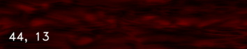
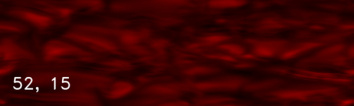
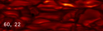
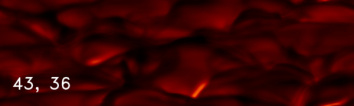
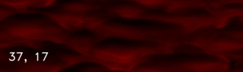
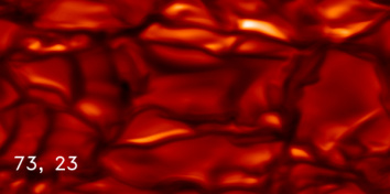
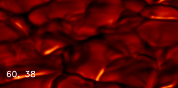
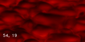
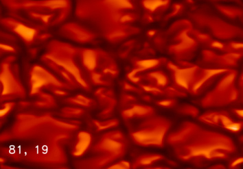
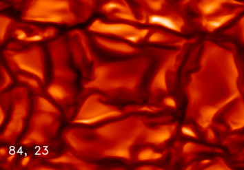
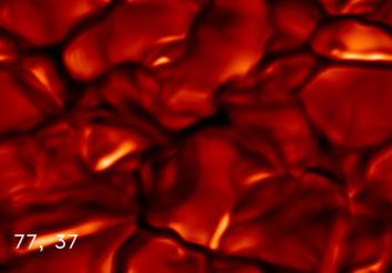
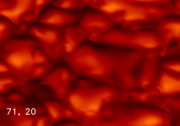
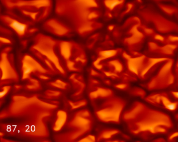
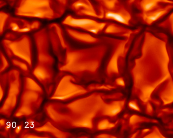
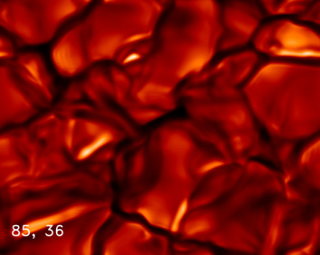
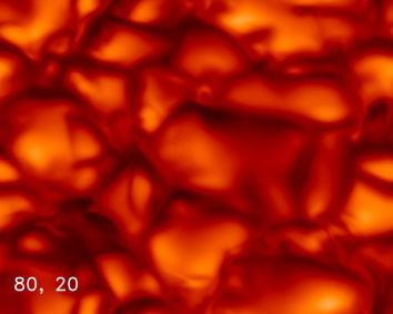
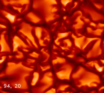
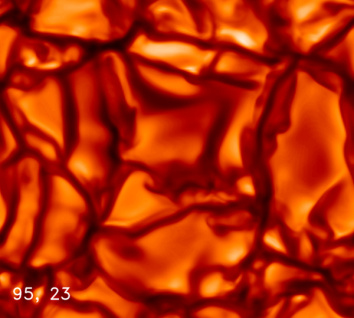
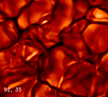
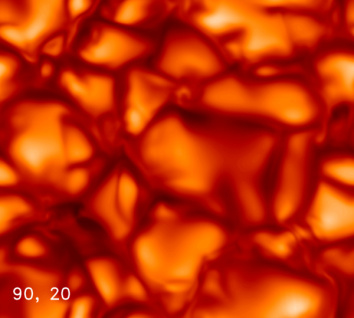
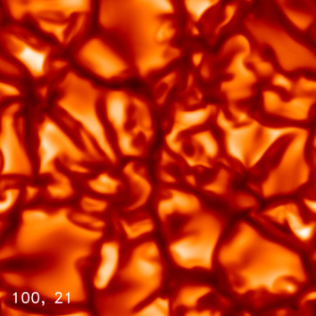
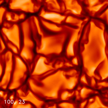
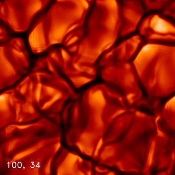
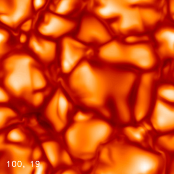
$8.0\,\left[\mathrm{Mm}\right]$                          $28.0\,\left[\mathrm{Mm}\right]$                          $2400.0\,\left[\mathrm{Mm}\right]$                         $1.4\,\left[\mathrm{Mm}\right]$

Figure 1: The emergent monochromatic intensity at $500\,\mathrm{nm}$ shown for eight $\mu$ angles: 0.2, 0.3, 0.5, 0.7, 0.8, 0.9, 1.0 (from top to down, respectively) and for a selection of stars: main-sequence, turnoff, K-giant, K-dwarf (from left to right, respectively) with solar metallicity. Furthermore, we indicated the normalized mean intensity and the intensity contrast (both in percent).

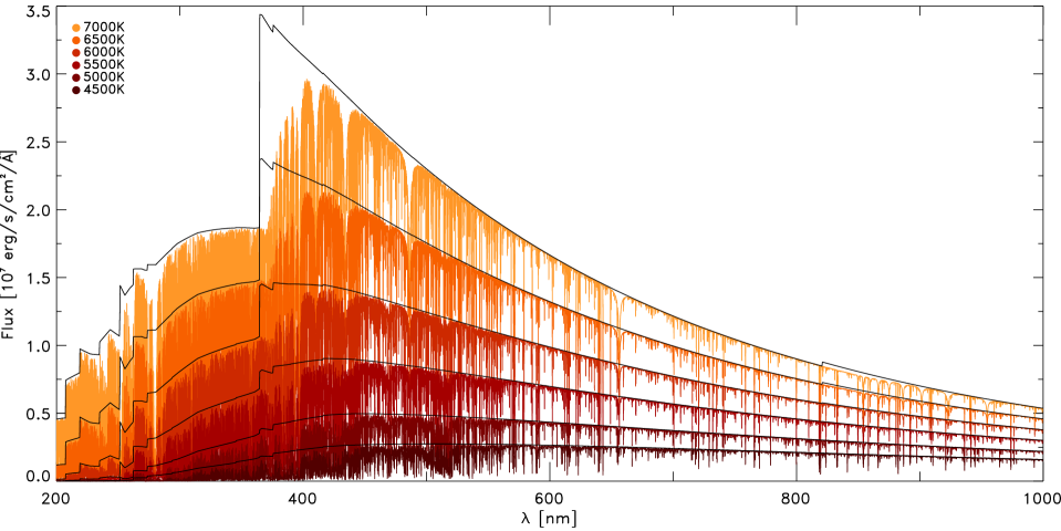
Figure 2: Spectral energy distribution vs. wavelength for models with $\log g=4.5$, $\left[\mathrm{Fe}/\mathrm{H}\right]=0.0$ and various $T_{\mathrm{eff}}$ (red/orange colors). The continuum fluxes are also shown (solid black lines).

Based on the 3D RHD models from the Stagger-grid, we computed a comprehensive library of full 3D synthetic spectra. Therefore, we used the Optim3D-code (see Chiavassa et al. 2009, 2010, for further details), which is a post-processing 3D radiative transfer code that assumes local thermodynamic equilibrium ($S_{\lambda}\left(T\right)=B_{\lambda}\left(T\right)$). The code considers the realistic velocity field due to convective motions present in the 3D RHD simulations, thereby taking Doppler broadening and shifts into account. Optim3D employs pre-tabulated extinction coefficients are the same as in the MARCS and Stagger codes, thereby accounting for continuous and sampled line opacities (Gustafsson et al. 2008). We assumed the latest solar composition by Asplund et al. (2009) consistently in Optim3D as in the 3D RHD simulations performed with the Stagger-code. In contrast to the RHD-code, the spectral synthesis code computes the large number of wavelength points with $N_{\lambda}=105\,767$ explicitly, thereby raising the computational costs enormously. We achieve a wavelength resolution with a constant sampling rate of $\lambda/\Delta\lambda=20\,000$, however, we cover a broad range with $\lambda=1010.0$ to $199\,960.0\,\mathring{A}$. We apply $N_{t}=10$ snapshots for each simulation, while we keep the horizontal mesh resolution fixed with $N_{xy}=240$. Four (equidistant) azimutal $\phi$-angles are considered ($N_{\phi}=4$), while the center-to-limb resolution is resolved higher with nine $\mu$-angles besides the disk-center ($\mu=0.01,0.05,0.10,0.20,0.30,0.50,0.70,0.80,0.90,1.00$). After carrying out tests with more $\mu$-angles, we found the ten chosen angles being sufficient to resolve the limb darkening accurately at lower computational costs. The strongest decline in the limb darkening is usually found towards the limb, therefore, we decided to resolve the limb more instead of equidistant $\mu$-angles. As shown by Hayek et al. (2012) the numerical resolution of our 3D RHD models and the resolution for the spectral flux computations are sufficient to predict realistic observed limb darkening laws accurately. The synthetic spectra will be discussed in a separate work (Chiavassa et al. in perp.).

We show an overview of spatially resolved intensity maps with different inclined $\mu$ angles for a selection of distinct stellar parameters (see Fig. 1). These exhibit the typical granulation pattern of cool stars due to convection. The bright, bulk regions are the hotter upflowing granules, which are interspersed with the dark intergranular downdrafts. From the disk-center towards the limb, the brightness is diminishing significantly, and the intensity contrast is also slightly dropping. Moreover, one can also obtain that bright features are often highly angle dependent.

In Fig. 2, we show a subset of the resulting averaged synthetic fluxes in the range $2000-10\,000\,\mathring{A}$ for a number of dwarfs with solar metallicity. Furthermore, we show also the continuum fluxes as well, and one can discern spectral absorption features, the prominent one being the Balmer lines (indicated in the figure). For higher $T_{\mathrm{eff}}$ the continuum flux is increasing, while individual spectral absorption features are changing as well.

3 Deriving the limb darkening

The variation of the inclination of the line of sight from the disk-center is parameterized with the projected polar angle, $\mu=\cos\theta$, where $\theta$ is the angle between the line of sight and the direction of the emergent radiation. Therefore, the disk-center is depicted with $\mu=1$, while $\mu=0$ is the limb. The limb darkening law is expressed as the variation in intensity with $\mu$-angle that is normalized to the disk-center, i.e. $I\left(\mu\right)/I\left(1\right)$. The resulting monochromatic intensity depends on the horizontal position $x$ and $y$, the viewing angles $\phi$ and $\mu$ and the time, $t$, thus $I_{\lambda}\left(x,y,\mu,\phi,t\right)$. In order to yield the mean monochromatic intensity $\left\langle I_{\lambda}\right\rangle\left(\mu\right)$ from the latter, we average the intensity first spatially, then over the azimutal angles, and finally over all time steps, i.e.

$$\left\langle I_{\lambda}\right\rangle\left(x,y,\mu,\phi,t\right) = \frac{1}{N_{t}}\sum_{t}\frac{1}{N_{\phi}}\sum_{\phi}\frac{1}{N_{x}N_{y}}\sum_{x,y}I_{\lambda}\left(x,y,\mu,\phi,t\right).$$

As next, we compute the inclination-dependent total emergent intensity $I\left(\mu\right)$ by integrating the mean monochromatic intensity $\left\langle I_{\lambda}\right\rangle$ over all wavelength points with

$$I\left(\mu\right) = \int\left\langle I_{\lambda}\right\rangle\left(\mu\right)\,d\lambda.$$

Then, the total surface brightness variation can be easily derived by normalizing the angular intensities with the disk-center value, $I_{\mu}/I_{1}$, and we can fit the various (bi-parametric) functional bases,

$$I_{\mu}/I_{1} = 1-u\left(1-\mu\right),$$ (1)

$$I_{\mu}/I_{1} = 1-a\left(1-\mu\right)-b\left(1-\mu\right)^{2},$$ (2)

$$I_{\mu}/I_{1} = 1-c\left(1-\mu\right)-d\left(1-\sqrt{\mu}\right),$$ (3)

$$I_{\mu}/I_{1} = 1-e\left(1-\mu\right)-f\mu\ln\mu,$$ (4)

$$I_{\mu}/I_{1} = 1-g\left(1-\mu\right)-h/\left(1-e^{\mu}\right),$$ (5)

which are the linear (Eq. 1), quadratic (Eq. 2), square root (Eq. 3), logarithmic (Eq. 4) and exponential (Eq. 5) limb darkening law. Also the three-parameter non-linear limb darkening law,

$$I_{\mu}/I_{1} = 1-a_{2}(1-\mu)-a_{3}(1-\mu^{3/2})-a_{4}(1-\mu^{2}),$$ (6)

introduced by Sing (2010) is also considered. However, we recommend the use of the standard four-parameter non-linear functional basis (Eq. 7) introduced by Claret (2000), which is the default limb darkening law in the present study. The four-parameter power law is the fourth order Taylor-series expansion in $\mu^{1/2}$ given by

$$I_{\mu}/I_{1} = 1-\sum_{k=1}^{4}a_{k}\left(1-\mu^{k/2}\right),$$ (7)

This functional basis conserves the flux to better than $0.05\,\%$ (see Claret 2000). In order to fit the LDC, we applied the Levenberg-Marquardt least-square minimization, since Claret (2000) showed that this fitting method performs best.

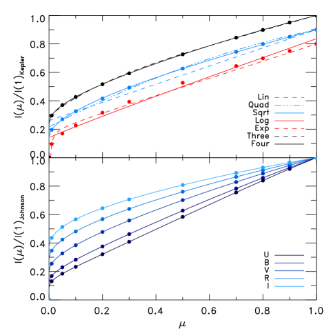
Figure 3: Solar intensity distribution vs. $\mu$-angle for different limb darkening laws in the Kepler filter (top) and different bands from the Johnson filters (bottom panel). The 3D results are indicated with filled circles. In the top panel the blue and red lines are shifted by $0.1$ and $0.2$ respectively, while the black lines are unshifted.

Table 1: The precision of the functional fits for the different limb darkening laws (see text for details).

Value	Lin	Quad	Sqrt	Log	Three	Four
$\overline{\chi^{2}}$	1.53	1.20	0.72	13.38	2.13	2.35$\times 10^{-6}$
$\overline{\max\delta}$	1.20	1.79	1.56	2.00	1.37	1.65$\times 10^{-3}$
$\overline{\mu}$	0.07	0.05	0.05	0.08	0.06	0.10

To illustrate the performance of the individual functional basis we show in Fig. 3 (top panel) the limb darkening laws of the solar simulation seen in the Kepler filter. The two-coefficient laws are obviously rather inadequate and show the largest deviations at the limb ($\mu\sim 0.0$), in particular the linear, quadratic, logarithmic and exponential law (Eqs. 1, 2, 4 and 5), while the square root law (Eq. 3) exhibits a rather good match (it is already known that the square root law performs better for hotter stars, while for cooler stars the quadratic law is better see Claret 2000). The three-parameter functional basis (Eq. 6) is performing well, however, it mismatches the limb rather significantly. The standard four-parameter non-linear power law (Eq. 7) is an excellent functional basis, and due to its versatility the fits result in extreme small residuals. In order to depict the precision of the individual laws quantitatively, we list the average $\chi^{2}$, average maximal relative deviation and average location of the latter from all stellar models in Table 1. The four-parameter law performs for all stellar parameters significantly much better than any other limb darkening law, therefore, we will discuss subsequently the latter only.

We consider a number of broad band filters $b$ by convolving the response function $S_{\lambda}$, which considers the transmission of the filter $b$, with the integration of the intensity,

$$I_{b}\left(\mu\right) = \int S_{\lambda}\left\langle I_{\lambda}\right\rangle\left(\mu\right)\,d\lambda.$$

We applied multiple standard broad band filters taken from the SYNPHOT package, which comprises Bessel (JHK), Johnson (UBVRI) and Strömgren (uvby). Additionally we considered individual important instruments with CoRoT, Kepler, Mauna Kea (JHKLM), SDSS (ugriz) and HST (ACS, STIS). Furthermore, the complete grid of spectra will be made available online, such that limb darkening from different filters or wavelength bands can be derived. In Fig. 3 (bottom panel) we show the five different Johnson filters for the solar model. The brightness distribution and its curvature are becoming more enhanced towards higher wavelength from the ultra-violet to the infra-red, which is a general feature for all stellar parameters. The optical depth and the temperature gradient are dependent on the considered wavelength, since radiation at higher wavelength is emerging from higher geometrical depth.

4 Limb darkening

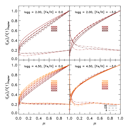
Figure 4: Disk-center normalized intensity, $I\left(\mu\right)/I\left(1\right)$, against the inclination, $\mu$, in the Kepler filter showing the limb darkening for different stellar parameters. Furthermore, we illustrate also the 1D ATLAS predictions for comparison (dashed lines), and the deviations $\Delta=1\mathrm{D}-3\mathrm{D}$ (dashed dotted lines), which are enhanced by a factor of $2$ and shifted by $+0.2$ for clarity.

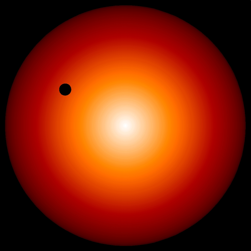
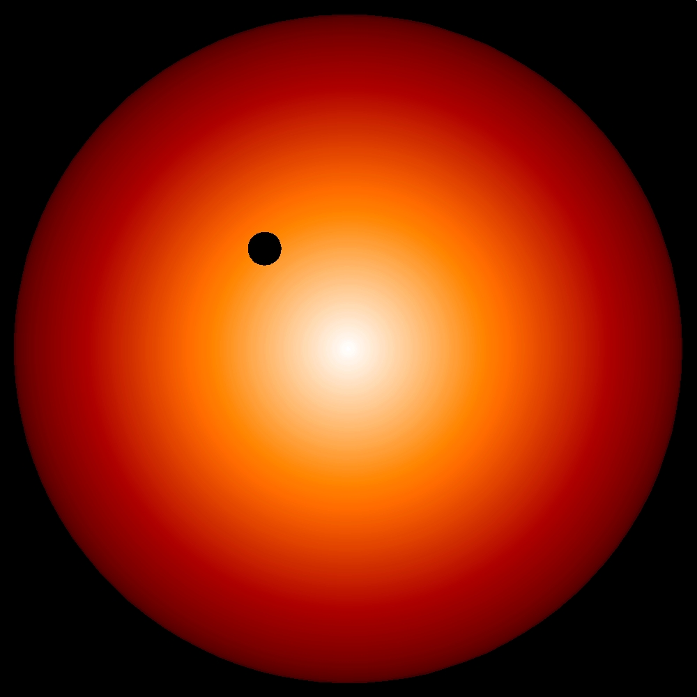
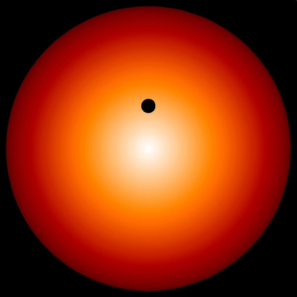
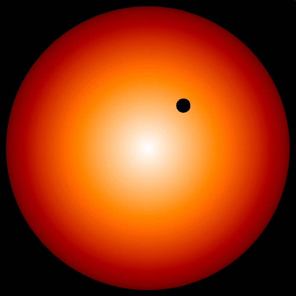
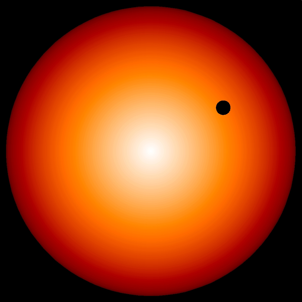
Figure 5: Synthetic stellar disks for stars with $\log g=4.5$, $\left[\mathrm{Fe}/\mathrm{H}\right]=0$, and increasing $T_{\mathrm{eff}}$ from $4500\,\mathrm{K}$ to $6500\,\mathrm{K}$ (from left to right) seen in the Kepler filter, and including a transiting exoplanet with $p=0.05$ with progressing transit phase. Note the brighter limb towards higher $T_{\mathrm{eff}}$.

The emergent radiative intensity of stars decreases almost linear monotonically from the center to the edge, until it drops-off sharply close to the limb ($\mu\sim 0.1$), which is known as limb darkening and can be observed in the Sun. The radiation at disk-center emerges from lower depths, while towards the limb one observes light from higher layers, where the temperature stratification has dropped very quickly, hence lower (darker) brightness ($I\propto T^{4}$). We mention that the limb darkening has obvious boundary constraints being that the intensity is maximal with $I\left(\mu=1\right)=1$ and minimal with $I\left(\mu=0\right)\simeq 0$. Furthermore, we note briefly that the variation of the limb darkening with stellar parameter depends also on the considered filter, and the results can differ significantly (Fig. 3).

In Fig. 4, we show an overview of different limb darkening variations for various stellar parameters. One finds in general that the variations are rather smooth and systematic, and the largest differences are given close to the limb ($\mu\sim 0.2$), however, the variations with $T_{\mathrm{eff}}$ and $\log g$ are distinctive for different metallicities. For higher $T_{\mathrm{eff}}$ the decline in brightness exhibits a more pronounced convex curvature between $\mu=0.2-0.7$, while at cooler ones it is close to a linear drop. Therefore, hotter models end up with brighter intensities towards the limb around $\mu\sim 0.2$ and a steeper drop beyond. For instance for dwarfs with solar-metallicity we find $I_{0.2}/I_{1}=0.4-0.6$ for $T_{\mathrm{eff}}=4500-7000\,\mathrm{K}$. In order to illustrate the relative brightening at the limb for hotter dwarfs with solar metallicity, we show synthetic stellar disks in Fig. 5 with higher $T_{\mathrm{eff}}$. Towards giants (lower $\log g$) the brightness is higher than for dwarfs, however the changes are more subtle compared to the effective temperature. At lower metallicity, we find the differences with $T_{\mathrm{eff}}$ between metal-poor dwarfs ($\log g=4.5,$ $\left[\mathrm{Fe}/\mathrm{H}\right]=-3$) being distinctively smaller, so that a pronounced curvature is given even for the coolest effective temperature (compare bottom panels in Fig. 4). In fact, we find basically no increase with $T_{\mathrm{eff}}$ around $\mu\sim 0.2$ ($I_{0.2}/I_{1}=0.59-0.61$). As we show further down, the $T$-insensitivity of the limb darkening at $\left[\mathrm{Fe}/\mathrm{H}\right]=-3$ arises due to the temperature gradient. Claret (2000) had also found an enhanced curvature at lower metallicity with 1D models. The hottest and most metal-poor dwarfs are the brightest at the edge, and the sharp drop is the steepest. Furthermore, we note that the center-to-limb variation curves for metal-poor models cross the corresponding ones for solar-metallicity models with otherwise the same stellar parameters ($T_{\mathrm{eff}}$), with the exception of the models at high $T_{\mathrm{eff}}$, however, this is not the case towards higher $T_{\mathrm{eff}}$. On the other hand, the metal-poor giants are more similar to the solar-metallicity case, and exhibit also a clear $T_{\mathrm{eff}}$ sensitivity.

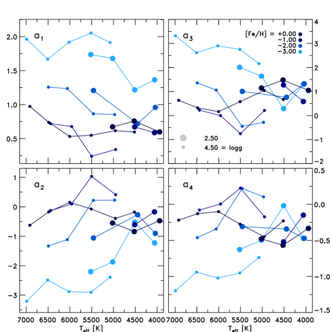
Figure 6: The four coefficients for the four-parameter non-linear limb darkening law (Eq. 7) predicted in the Kepler filter from 3D RHD models for different stellar parameters.

As next, we want to discuss the individual coefficients for the four-parameter limb darkening law (Eq. 7). Therefore, we show in Fig. 6 the four coefficients for different $T_{\mathrm{eff}}$ and $\left[\mathrm{Fe}/\mathrm{H}\right]$ and $\log g=4.5,2.0$. Towards higher $T_{\mathrm{eff}}$ both coefficients, $a_{2}$ and $a_{4}$, are increasing until $6000\,\mathrm{K}$, then above they decrease, while the coefficients $a_{1}$ and $a_{3}$ vary the opposite at solar metallicity. For lower $\left[\mathrm{Fe}/\mathrm{H}\right]$ the $T$-dependence is inverted for $a_{k}$ and the even coefficients, $a_{2}$ and $a_{4}$, are decreasing, and the odd ones, $a_{1}$ and $a_{3}$, are increasing. Another aspect worthy of attention is the correlation between the coefficients with half-integer exponents in $\mu$ ($a_{1}$ and $a_{3}$), and integer one ($a_{2}$ and $a_{4}$) with $T_{\mathrm{eff}}$ and $\left[\mathrm{Fe}/\mathrm{H}\right]$ (compare left with right panels in Fig. 6). In the Kepler filter we find the correlations to amount with $C\left[a_{1},a_{3}\right]=0.82$ and $C\left[a_{2},a_{4}\right]=0.91$ for all stellar parameters. Furthermore, the half-integer exponents anti-correlate with the integer ones (compare top with bottom panels in Fig. 6). While the distant coefficients are less anti-correlated with $C\left[a_{1},a_{4}\right]=-0.76$, we find the anti-correlation between the successive coefficients being much tighter with $C\left[a_{1},a_{2}\right]=-0.95$ and $C\left[a_{3},a_{4}\right]=-0.99$. Claret (2000) noted also correlations between the coefficients. The coefficients $a_{k}$ of the four-parameter law can be decomposed and considered individually. Then the integer exponents with the coefficients $a_{2}$ and $a_{4}$ are leading to a linear and quadratic polynomial respectively, which are describing the general slope of the limb darkening. On the other hand, the half-integer exponents with the coefficients $a_{1}$ and $a_{3}$ are square root like functions, and are responsible for the curvature towards the limb.

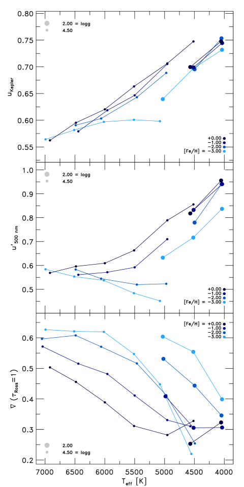
Figure 7: The coefficient $u$ of the linear limb darkening law (Eq. 1) in the Kepler filter (top) and the approximation $u_{500\,\mathrm{nm}}^{{}^{\prime}}$ from Eq. 8 (middle) and temperature gradient at the optical surface (bottom panel) vs. $T_{\mathrm{eff}}$ for $\log g=2.0,\,4.5$ and different $\left[\mathrm{Fe}/\mathrm{H}\right]$.

The coefficient $u$ for the linear limb darkening law (Eq. 1) is rather crude, however, it has the major advantage of simplicity, since the linear law reduces the complex shape of the limb darkening into a single value. We display in Fig. 7 $u$ against $T_{\mathrm{eff}}$ for different stellar parameters (top panel). A larger value in $u$ relates to a steeper drop in intensity and indicate lower brightness at the limb, and a lower value for $u$ results in brighter limbs (see Eq. 1). The coefficient $u$ is mainly sensitive to the effective temperature and is decreasing with higher $T_{\mathrm{eff}}$, and for different $\log g$ and $\left[\mathrm{Fe}/\mathrm{H}\right]$ the differences are rather small. As a remark we note that the linear coefficients $a$ and $c$ from Eqs. 2 and 3 are similar, while the quadratic and square root coefficients, $b$ and $d$, behave oppositely and increase for higher $T_{\mathrm{eff}}$ (not shown). The values for $u$ ranges from 0.56 to 0.77 in the Kepler filter, which would yield $I=0.44$ and $0.23$ at the limb ($\mu=0$) respectively (the global range in $u$ is from $0.03$ to 1.05).

With a linear approximation of the Planck function one can derive the slope of the linear limb darkening law, $u$ (e.g. Gray 2005; Hayek et al. 2012), which depends primarily on the temperature gradient at the optical surface and is given by

$$u_{\lambda}^{{}^{\prime}} \approx \frac{\log e}{B_{\lambda}\left(T\left(\tau_{\lambda}=1\right)\right)}\frac{dB_{\lambda}}{dT}\Big{|}_{\tau_{\lambda}=1}\frac{dT}{d\log\tau}\Big{|}_{\tau_{\lambda}=1}$$ (8)

The approximation implies that a steeper temperature gradient at the optical surface will lead to stronger (steeper) limb darkening (larger $u$). In Fig. 7 (middle panel) we show also $u_{500\,\mathrm{nm}}^{{}^{\prime}}$ considered at the optical surface ($\tau=1$) vs. $T_{\mathrm{eff}}$, and we find $u_{500\,\mathrm{nm}}^{{}^{\prime}}$ to correlate well with $u$ (top panel). Also, similar as given in $u$, we find $u_{500\,\mathrm{nm}}^{{}^{\prime}}$ being $T$-insensitive for dwarf models with very low metallicity ($\left[\mathrm{Fe}/\mathrm{H}\right]=-3$), which arises from the temperature gradient term $dT/d\log\tau_{\lambda}$ in Eq. 8. The intensity is given by the source function and the lost radiation, which is stated by the radiative transfer eq., $dI_{\lambda}/d\tau_{\lambda}=S_{\lambda}-I_{\lambda}$. Under the assumption of LTE, the source function can be approximated with the Planck function at the local temperature, $S_{\lambda}\left(T\right)=B_{\lambda}\left(T\right)$. Therefore, the variation of the intensity with $\mu$ is sensitive to the temperature structure and in particular the temperature gradient. In Fig. 7 we show also the temperature gradient, $\@vec{\nabla}=d\ln T/d\ln p_{\mathrm{tot}}$, considered at the optical surface (bottom panel). For lower metallicity the range in temperature gradient is enhanced, which is very similar to the intensity contrast. We had already mentioned the enhancement of the intensity contrast and temperature gradient at lower metallicity in Paper I. We find the reason for the enhancement being the lack of metals that are usually the most important electron donors for the formation of $\mathrm{H}^{-}$, which is the dominating opacity source (see Nordlund & Dravins 1990). Therefore, in metal-poor models, the main contribution of electrons arises from the ionization of hydrogen. This is the reason for the strong enhancement of the of temperature gradient towards $T_{\mathrm{eff}}=6000\,\mathrm{K}$ with $\left[\mathrm{Fe}/\mathrm{H}\right]=-3$, which is the reason for the $T$-insensitivity of $u$ and the limb darkening that we found for metal-poor dwarfs (see Fig. 4).

5 Transit light curves

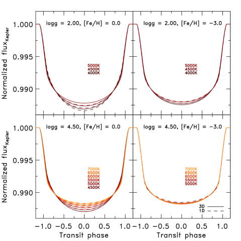
(a)

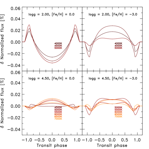
(b)

Figure 8: Left figure: transit light curve vs. transit phase with $p=0.1$ in the Kepler filter for different stellar parameters. The predictions from the 1D ATLAS models are also included (dashed lines). Right figure: relative deviations in the transit light curve with $p=0.1$ between 3D atmosphere models and 1D ATLAS models given in $\%$. The difference is $\delta=1\mathrm{D}/3\mathrm{D}-1$.

During exo-solar planet transits the planet eclipses its host star in the line of sight to earth, thereby diminishing the emergent intensity and leaving a characteristic imprint in the observed light curve. Theoretical light curve predictions are described by two main parameters, namely the ratio of the radii of planet and parent star, $p=r_{\mathrm{planet}}/r_{\mathrm{star}}$, and the normalized separation of the centers, $z=d/r_{\mathrm{star}}$, with $d$ being the center-to-center distance of the two occulting bodies. For computing the theoretical transit light curves, we used the publicly available code by Mandel & Agol (2002). In Fig. 8a, we show light curves with $p=0.1$, i.e. for the case that the radius of the planet is $1/10$ of the star, in the Kepler filter for the same LDC as discussed in Sec. 4. Then one can extract that the dwarfs with solar-metallicity exhibit for higher $T_{\mathrm{eff}}$ light curves with a more rectangular shaped feature, where the transit center is shallower and the width of the transit is broader than lower $T_{\mathrm{eff}}$. The giant models show similar features with $T_{\mathrm{eff}}$ for both $\left[\mathrm{Fe}/\mathrm{H}\right]$. On the other hand, the metal-poor dwarfs are similarly box-shaped and do not alter much for lower effective temperatures. The limb of the intensity distribution will shape the ingress and egress of the light curve, e.g. when the limb darkening would be a step function ($a_{2}\simeq 0.$ and $a_{k}=0.$), then the light curve would be entirely rectangular. A straight linear dropping intensity distribution ($a_{2}=1$ and $a_{k}=0.$) results in a more elliptical shape with a narrow width, while a curved square root drop ($a_{1}=1$ and $a_{k}=0.$) would lead to an evenly circular shaped light curve. Therefore, we caution for the use of limb darkening laws that are incapable of rendering the drop-off at the limb, such as the bi- and three-parametric laws, since these will introduce inevitably systematic errors in the theoretical transit light curves. Mandel & Agol (2002) found in a comparison between the quadratic and the four-parameter non-linear power law (with $p=0.1$) differences by $3\,\%$! Furthermore, the depth of the transit light curve depends primarily on the ratio of planet to host $p$. For larger $p$ the light curves are increasingly deeper at the center, since more stellar light is effectively blocked during the transition due to a larger surface ratio of the planet. The limb darkening is also sensitive to the considered wavelength-regime (see Fig. 3). Therefore, the transit light curve will be different depending on the actual considered broad band filter, which samples its specific range in $\lambda$. We find in general that the light curve is towards lower wavelength (ultra-violet) systematically more convex shaped with a deeper center and more slender width, while towards higher wavelength (infra-red) the light curve is more box-shaped with shallower centers and broader width. We note that a multi-band photometry approach states a solution to this issue (see Knutson et al. 2007).

6 Comparison with results from 1D models

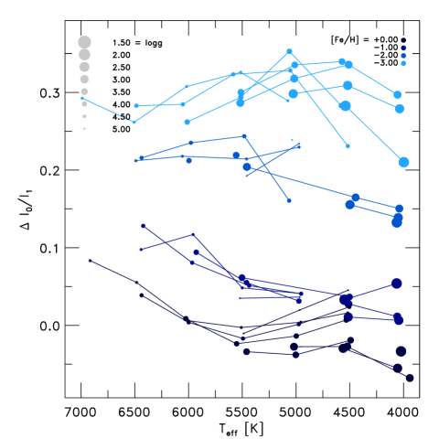
Figure 9: Overview of the maximal relative difference in the limb darkening compared between 1D and 3D against $T_{\mathrm{eff}}$ with the Kepler filter. The relative deviations are retrieved by $\Delta=1\mathrm{D}-3\mathrm{D}$

The ATLAS models are the widest applied 1D atmosphere models for retrieving LDC, since its grid covers the broadest range in stellar parameters leading to seamless coverage. The differences between the 1D and 3D models arise mainly from the differences in the temperature stratification, in particular, the temperature gradients.

For the comparison, we show in Fig. 4 also the limb darkening derived from 1D MLT models from the ATLAS grid (see Sing 2010). To ensure consistency the four-parameter non-linear laws for 1D models are also shown in the Kepler filter. The 1D dwarf models with solar metallicity exhibit similar increasing curvatures for higher $T_{\mathrm{eff}}$ as given by the 3D models, only the 1D models are slightly brighter than the 3D, except for the coolest one ($4500\,\mathrm{K}$). In the case of giants the 1D limb darkening is distributed at much lower and also more linear intensities. The limb of the metal-poor 1D models lacks of a similar smooth sharp drop-off that is given in the 3D models, instead they depict a rather discontinuous behavior at the limb, which is doubtful to be correct. For metal-poor models it is known that the enforcement of radiative equilibrium is leading to an overestimation of the temperature stratification in the upper layers due to lack of spectral line absorption (see Asplund et al. 1999; Collet et al. 2007). The radiation at the limb is emerging from higher layers, therefore, the deviations at the limb are consistent (see also Paper I).

The largest deviations are usually found at the limb, since some of the 1D models depict an almost linear run at the edge, while the 3D models exhibit a comparably smooth drop-off at the limb. In Figure 9, we show the deviations at the limb, $\Delta I_{0}/I_{1}$, between the 1D and 3D limb darkening predictions. The differences increase significantly towards lower metallicity. Therefore, we advise the use of 3D limb darkening coefficients in particular for metal-poor stars.

We display the relative differences in the transit light curve between the 3D and 1D predictions in Fig. 8b. Similar to the findings of Hayek et al. (2012), we find a characteristic shape in the residuals with two extrema that are usually of opposite sign. One being at the ingress and egress phase, which arises from differences at the limb, and the other one taking place at the disk-center. We found in Sec. 4 the 1D models being brighter than the 3D limb darkening, except for the giants at solar-metallicity. The transit light curves for the 1D models are similarly brighter at the disk-center and dimmer at the transit phase edges for all models, only for the solar-metallicity giants it is the opposite. However, the maximal residuals are relatively small with a global maximum of $\sim 0.04\,\%$ in the transit light curve.

Since the differences in the transit light curves between 3D and 1D are rather small, the expected differences in transit parameters are also small. Hayek et al. (2012) determined a larger (smaller) radius of the exoplanet HD 209458b (HD 189733b) by 0.2 % in the wavelength region between 2900 and 5700 $\mathring{A}$. Hence, a reanalysis of the observed transit light curves with our LDC might change the transit parameters less than a percent.

7 Conclusions

We derived on the basis of the Stagger-grid, a large grid of 3D RHD atmosphere models, the limb darkening coefficients for the various bi-parametric and non-linear limb darkening laws. The four-parameter non-linear power law introduced by Claret (2000) is the only limb darkening law that is sufficiently versatile to express the intensity distribution with an excellent accuracy, while all other limb darkening laws are insufficient, in particular at the limb. Therefore, we recommend the use of the four-parameter functional basis only, in particular for the comparison with high-precision measurements in the hunt of extrasolar planets. We discussed the limb darkening in the Kepler filter for various stellar parameters, and outlined systematical variations that exposed the complex changes of the brightness distribution, in particular with the effective temperature. We compared also our new LDC with predictions from widely used 1D ATLAS models, and the largest differences are given towards the limb. The 1D models are often brighter than 3D predictions, only for giant models with solar-metallicity we find opposite differences. Furthermore, we displayed the systematic (anti-)correlations between the coefficients $a_{k}$ between half-integer and integer exponents of the four-parameter law. We found the coefficient of linear limb darkening law, $u$, to scale with the temperature gradient and the Planck function. Theoretical transit light curves indicate similar systematical differences between 1D and 3D as the limb darkening variations implied, which are relatively small. However, as observations indicate (Knutson et al. 2007; Hayek et al. 2012), these can be measured with high-precision observations. Therefore, we advise to use of of the new LDC.

Appendix A Table with the limb darkening coefficients

In Table 2 we listed a subset of the limb darkening coefficients for F, G, and K main-sequence stars. The full table is available at CDS.

Table 2: Limb darkening coefficients derived from 3D RHD models in the Kepler filter for different stellar parameters (Cols. 1,2,3). The linear (Col. 4), quadratic (Cols. 5,6), square root (Cols. 7,8) and four-parameter non-linear laws (Cols. 9,10,11,12) are listed.

$T_{\rm{eff}}$	$\log g$	[Fe/H]	$u$	$a$	$b$	$c$	$d$	$a_{1}$	$a_{2}$	$a_{3}$	$a_{4}$
4532	3.50	+0.0	0.73505	0.58775	0.17369	0.47757	0.33638	0.77661	-0.80075	1.38617	-0.50608
4997	3.50	+0.0	0.69317	0.51184	0.21380	0.40246	0.37978	0.63495	-0.46625	1.10377	-0.46910
5552	3.50	+0.0	0.63205	0.37638	0.30146	0.23583	0.51764	0.52385	0.09984	0.29682	-0.16943
6025	3.50	+0.0	0.57909	0.27389	0.35988	0.08275	0.64845	0.70830	0.00368	-0.03424	0.06155
4504	4.00	+0.0	0.74641	0.58971	0.18481	0.47456	0.35520	0.76201	-0.69272	1.24804	-0.44840
4974	4.00	+0.0	0.69924	0.51916	0.21233	0.40603	0.38305	0.69226	-0.60023	1.22834	-0.50452
5493	4.00	+0.0	0.64892	0.42136	0.26832	0.29549	0.46173	0.54134	-0.07649	0.58178	-0.28535
5999	4.00	+0.0	0.61169	0.34095	0.31926	0.18721	0.55457	0.53991	0.17288	0.08752	-0.06136
6437	4.00	+0.0	0.57175	0.26414	0.36271	0.07584	0.64788	0.80623	-0.39503	0.52466	-0.19731
5767	4.44	+0.0	0.63905	0.39256	0.29064	0.25352	0.50367	0.58503	-0.10226	0.53712	-0.25796
4518	4.50	+0.0	0.74748	0.58106	0.19623	0.46824	0.36481	0.59750	-0.17959	0.66723	-0.22919
4955	4.50	+0.0	0.70630	0.52186	0.21747	0.41223	0.38419	0.61695	-0.39597	1.04387	-0.44957
5509	4.50	+0.0	0.66324	0.43841	0.26511	0.31192	0.45897	0.54929	-0.07493	0.57716	-0.27516
6002	4.50	+0.0	0.62040	0.35566	0.31221	0.20713	0.53998	0.53192	0.15042	0.16292	-0.10095
6483	4.50	+0.0	0.59534	0.28054	0.37119	0.09313	0.65611	0.73898	-0.17219	0.31894	-0.12921
6915	4.50	+0.0	0.56230	0.20662	0.41939	-0.01686	0.75662	0.97382	-0.62622	0.63240	-0.21903
4515	5.00	+0.0	0.74272	0.52349	0.25852	0.38093	0.47270	0.66450	-0.13643	0.51088	-0.16603
4965	5.00	+0.0	0.72911	0.53095	0.23365	0.42084	0.40274	0.47629	0.08613	0.51634	-0.25122
5488	5.00	+0.0	0.66477	0.43757	0.26789	0.31734	0.45389	0.47390	0.09151	0.45732	-0.25382
5996	3.50	-2.0	0.59147	0.23859	0.41607	-0.00987	0.78563	1.40907	-1.73174	1.75496	-0.59484
5063	4.00	-2.0	0.67569	0.30132	0.44143	0.09182	0.76280	0.53808	0.75966	-0.74362	0.27944
5481	4.00	-2.0	0.63979	0.22783	0.48574	-0.03935	0.88726	1.21877	-0.91653	0.84285	-0.26340
5977	4.00	-2.0	0.59856	0.20852	0.45991	-0.06036	0.86084	1.43622	-1.63025	1.57506	-0.52309
6437	4.00	-2.0	0.56859	0.17828	0.46022	-0.09412	0.86578	1.39622	-1.46391	1.26974	-0.37546
5784	4.44	-2.0	0.62103	0.20358	0.49221	-0.06998	0.90276	1.30219	-1.15073	1.07186	-0.35042
4972	4.50	-2.0	0.68860	0.23125	0.53926	-0.03294	0.94265	0.85345	0.22723	-0.28352	0.10407
5460	4.50	-2.0	0.64309	0.20143	0.52075	-0.06477	0.92477	0.86507	0.21908	-0.44776	0.22070
6057	4.50	-2.0	0.60317	0.21858	0.45348	-0.03590	0.83491	1.23655	-1.11440	1.05958	-0.34213
6490	4.50	-2.0	0.59069	0.23563	0.41864	-0.00428	0.77730	1.25723	-1.33216	1.35739	-0.46197
4971	5.00	-2.0	0.66775	0.17879	0.57657	-0.10938	1.01532	1.02230	-0.12475	0.01055	-0.00136
5458	5.00	-2.0	0.64344	0.18595	0.53943	-0.07624	0.94022	0.66300	0.82112	-1.09008	0.44583